
Home / Advanced Excel / How to use Icon Sets in Excel (Conditional Formatting)
In Excel Conditional Formatting, there are icon sets that you can apply to data. These icon sets help to measure which value is lowest, highest, or at the mid.
There is a total of 20 pre-made icon sets in four categories that you can apply to the data.
Keyboard Shortcut to Open Icons Sets: Alt ⇢ H ⇢ L ⇢ I
Apply Icon Sets to a Data
- First, select the data and go to the home tab.
- From the home tab, click on the conditional formatting drop-down.
- After that, go to the “Icon Sets” option.
- In the end, select the icon set that you want to apply to the selected data.
Custom Rules to Apply Icon Sets
When you apply icon sets to data, Excel automatically creates a rule to apply. It decides which are the values in the lowest and highest, and in the middle. But you can decide these by yourself if you want. Open the icon sets and click on more rules.
This will open the new formatting rule dialog box (Keyboard Shortcut to Open Icons Sets: Alt ⇢ H ⇢ L ⇢ I ⇢ M).

By default, you have the type of rules based on percentage.

But there are four different ways to apply a rule for an icon set.
Use a Custom Numbers Range to Apply Icon Sets
In the following example, we have used a custom range of numbers:

- Green Up Arrow Icon for values above and equal to 1500.
- Yellow Bar Icon for values between 1500 and 1000.
- Red Bar Icon for values below 1000.
Apply Icon Sets Based on a Formula (value Depends on Another Cell)
In the following example, we have applied icon sets based on the values based on the cells C2 and C3. And in the type, we have used a formula.
And when you change any value from both cells the icon sets will also change on data.
Other Options with Icon Sets
- Reverse Icon Order: While applying icon formatting, you can change the order of the icons in reverse. So, the icon for the highest value will move to the lowest value.
- Show Icon Only: When you tick mark this option, this will hide the values from the range and show only the icons that you have.
- Icon Style: You can change the icon style. As you know we have 20 different styles to apply.
- Different Icons for Each Value: You can choose a different icon for each value. A different icon for middle, low, and high value.
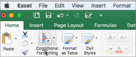
If you use Excel for Mac, well, all the options are the same there, just like Windows. The above steps will help you apply Icon Sets there as well.
More Tutorials
- Formulas in Conditional Formatting
- AUTO FORMAT Option in Excel
- Apply Accounting Number Format in Excel
- Apply Background Color to a Cell or the Entire Sheet in Excel
- Print Excel Gridlines (Remove, Shortcut, & Change Color)
- Add Page Number in Excel
- Apply Comma Style in Excel
- Apply Strikethrough in Excel
- Highlight Blank Cells in Excel
- Make Negative Numbers Red in Excel
- Cell Style (Title, Calculation, Total, Headings…) in Excel
- Change Date Format in Excel
- Highlight Alternate Rows in Excel with Color Shade
- Add Border in Excel
- Change Border Color in Excel
- Clear Formatting in Excel
- Copy Formatting in Excel
- Best Fonts for Microsoft Excel
- Hide Zero Values in Excel
⇠ Back to Advanced Excel Tutorials
Excel for Microsoft 365 for Mac Excel 2021 for Mac Excel 2019 for Mac Excel 2016 for Mac Excel for Mac 2011 More…Less
Important: Some of the content in this topic may not be applicable to some languages.
Data bars, color scales, and icon sets are conditional formats that create visual effects in your data. These conditional formats make it easier to compare the values of a range of cells at the same time.
 Data bars
 Color scales
 Icon sets
Format cells by using data bars
Data bars can help you spot larger and smaller numbers, such as top-selling and bottom-selling toys in a holiday sales report. A longer bar represents a larger value, and a shorter bar represents a smaller value.
-
Select the range of cells, the table, or the whole sheet that you want to apply conditional formatting to.
-
On the Home tab, click Conditional Formatting.

-
Point to Data Bars, and then click a gradient fill or a solid fill.
Tip: When you make a column with data bars wider, the differences between cell values become easier to see.
Format cells by using color scales
Color scales can help you understand data distribution and variation, such as investment returns over time. Cells are shaded with gradations of two or three colors that correspond to minimum, midpoint, and maximum thresholds.
-
Select the range of cells, the table, or the whole sheet that you want to apply conditional formatting to.
-
On the Home tab, click Conditional Formatting.
-
Point to Color Scales, and then click the color scale format that you want.
The top color represents larger values, the center color, if any, represents middle values, and the bottom color represents smaller values.
Format cells by using icon sets
Use an icon set to present data in three to five categories that are distinguished by a threshold value. Each icon represents a range of values and each cell is annotated with the icon that represents that range. For example, a three-icon set uses one icon to highlight all values that are greater than or equal to 67 percent, another icon for values that are less than 67 percent and greater than or equal to 33 percent, and another icon for values that are less than 33 percent.
-
Select the range of cells, the table, or the whole sheet that you want to apply conditional formatting to.
-
On the Home tab, click Conditional Formatting.
-
Point to Icon Sets, and then click the icon set that you want.
Tip: Icon sets can be combined with other conditional formats.
Format cells by using data bars
Data bars can help you spot larger and smaller numbers, such as top-selling and bottom-selling toys in a holiday sales report. A longer bar represents a larger value, and a shorter bar represents a smaller value.
-
Select the range of cells, the table, or the whole sheet that you want to apply conditional formatting to.
-
On the Home tab, under Format, click Conditional Formatting.
-
Point to Data Bars, and then click a gradient fill or a solid fill.
Tip: When you make a column with data bars wider, the differences between cell values become easier to see.
Format cells by using color scales
Color scales can help you understand data distribution and variation, such as investment returns over time. Cells are shaded with gradations of two or three colors that correspond to minimum, midpoint, and maximum thresholds.
-
Select the range of cells, the table, or the whole sheet that you want to apply conditional formatting to.
-
On the Home tab, under Format, click Conditional Formatting.
-
Point to Color Scales, and then click the color scale format that you want.
The top color represents larger values, the center color, if any, represents middle values, and the bottom color represents smaller values.
Format cells by using icon sets
Use an icon set to present data in three to five categories that are distinguished by a threshold value. Each icon represents a range of values and each cell is annotated with the icon that represents that range. For example, a three-icon set uses one icon to highlight all values that are greater than or equal to 67 percent, another icon for values that are less than 67 percent and greater than or equal to 33 percent, and another icon for values that are less than 33 percent.
-
Select the range of cells, the table, or the whole sheet that you want to apply conditional formatting to.
-
On the Home tab, under Format, click Conditional Formatting.
-
Point to Icon Sets, and then click the icon set that you want.
Tip: Icon sets can be combined with other conditional formats.
See Also
Highlight patterns and trends with conditional formatting
Need more help?
Want more options?
Explore subscription benefits, browse training courses, learn how to secure your device, and more.
Communities help you ask and answer questions, give feedback, and hear from experts with rich knowledge.
The “Conditional Formatting” button is hidden in the middle of the Home ribbon in Excel. Nonetheless, Conditional Formatting offers many options for visualizing your data. As the name already says, Excel can format your table depending on one or more conditions.
In this Excel tip, we will take a look at two options of applying a format to your cells depending on a condition: Color scales and icon sets.
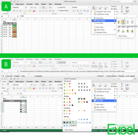
Conditional formatting with color scales
Color scales change the background color depending on the cell values. The default versions are the traffic light colors green, yellow and red. But there are also other options, e.g. blue-white-red (probably symbolizing cold to hot).
Figure (A) in the picture on the right hand side shows how to apply the color scale:
- Select a range of cells with values.
- Click on Conditional Formatting and then choose a scale under “Color Scales”.
Let’s say, we select the “Red-Yellow-Green Color Scale”. The cell containing the lowest value in your range will now get a dark green color. The cell with the highest value is dark red. All values in-between will have shades of green or red.
The animation above shows the opposite example: The lowest value get’s the red color and the highest value get’s green.
These color scales could be extremely useful for identifying and eliminating outliers.
Icon sets like traffic lights or harvey balls
Instead of just background colors, you can add small symbols to the cells depending on their values: Such ‘icon sets’ can be traffic lights (red, yellow, green), arrows or Harvey balls (those quarter/ half/ three quarter filled circles). Please compare to figure (B) in the picture above.
In our example, we want to show achievements by using Harvey balls. Basically, it’s the same process:
- Select the data you want to visualize.
- Click on Conditional Formatting on the Home ribbon.
- Select Harvey Balls under Icon Sets.
Excel will now automatically calculate in which quarter each value belongs and add the balls to each cell.
Remove conditional formatting rules but keep the colors
In some cases, you want to remove the conditional formatting rules but keep the format. For example, you’ve selected the background color depending on the values (see above). Now you want to keep the color, but either delete the values or even change the values.
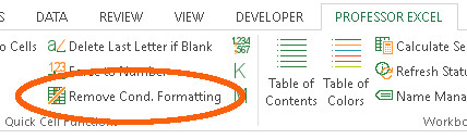
There is one very comfortable way: Use “Professor Excel Tools“:
- Select the cells having conditional formatting rules.
- Click on “Remove Cond. Formatting” within the Quick Cell Functions on the Professor Excel ribbon.
You can try the Excel add-in for free – no sign-up or installation needed. Just click the button below.

This function is included in our Excel Add-In ‘Professor Excel Tools’
(No sign-up, download starts directly)
Final thoughts
- Conditional Formatting can use a lot of performance, especially when using with formulas. In case your computer suddenly gets noticeably slower, you might want to reduce the conditional formatting to a minimum.
- Use Conditional Formatting only when it really improves your table. Don’t just use it for adding colors to your worksheet.
Further reading
You want to know more about conditional formatting? Please take a look at our articles:
- If you want to use a formula for defining the format of a cell, please refer to this article. The example in this article: How to highlight all Sundays on a calendar sheet.
- You want to hide all zero values? There are several methods – one of them is via conditional formatting.

Henrik Schiffner is a freelance business consultant and software developer. He lives and works in Hamburg, Germany. Besides being an Excel enthusiast he loves photography and sports.
Содержание
- Use data bars, color scales, and icon sets to highlight data
- Format cells by using data bars
- Format cells by using color scales
- Format cells by using icon sets
- Format cells by using data bars
- Format cells by using color scales
- Format cells by using icon sets
- Excel Icon Sets conditional formatting: inbuilt and custom
- Excel icon sets
- How to use icon sets in Excel
- How to customize Excel icon sets
- How to create a custom icon set in Excel
- How to set conditions based on another cell value
- Excel conditional formatting icon sets formula
- Excel conditional format icon set to compare 2 columns
- How to apply Excel icon sets based on another cell
- Excel conditional formatting icon sets based on text
- How to show only some items of the icon set
- How to add custom icon set to Excel
- Method 1. Add custom icons using Symbol menu
- Method 2. Add custom icons using virtual keyboard
Use data bars, color scales, and icon sets to highlight data
Important: Some of the content in this topic may not be applicable to some languages.
Data bars, color scales, and icon sets are conditional formats that create visual effects in your data. These conditional formats make it easier to compare the values of a range of cells at the same time.
Data bars
Color scales
Icon sets
Format cells by using data bars
Data bars can help you spot larger and smaller numbers, such as top-selling and bottom-selling toys in a holiday sales report. A longer bar represents a larger value, and a shorter bar represents a smaller value.
Select the range of cells, the table, or the whole sheet that you want to apply conditional formatting to.
On the Home tab, click Conditional Formatting.
Point to Data Bars, and then click a gradient fill or a solid fill.
Tip: When you make a column with data bars wider, the differences between cell values become easier to see.
Format cells by using color scales
Color scales can help you understand data distribution and variation, such as investment returns over time. Cells are shaded with gradations of two or three colors that correspond to minimum, midpoint, and maximum thresholds.
Select the range of cells, the table, or the whole sheet that you want to apply conditional formatting to.
On the Home tab, click Conditional Formatting.
Point to Color Scales, and then click the color scale format that you want.
The top color represents larger values, the center color, if any, represents middle values, and the bottom color represents smaller values.
Format cells by using icon sets
Use an icon set to present data in three to five categories that are distinguished by a threshold value. Each icon represents a range of values and each cell is annotated with the icon that represents that range. For example, a three-icon set uses one icon to highlight all values that are greater than or equal to 67 percent, another icon for values that are less than 67 percent and greater than or equal to 33 percent, and another icon for values that are less than 33 percent.
Select the range of cells, the table, or the whole sheet that you want to apply conditional formatting to.
On the Home tab, click Conditional Formatting.
Point to Icon Sets, and then click the icon set that you want.
Tip: Icon sets can be combined with other conditional formats.
Format cells by using data bars
Data bars can help you spot larger and smaller numbers, such as top-selling and bottom-selling toys in a holiday sales report. A longer bar represents a larger value, and a shorter bar represents a smaller value.
Select the range of cells, the table, or the whole sheet that you want to apply conditional formatting to.
On the Home tab, under Format, click Conditional Formatting.
Point to Data Bars, and then click a gradient fill or a solid fill.
Tip: When you make a column with data bars wider, the differences between cell values become easier to see.
Format cells by using color scales
Color scales can help you understand data distribution and variation, such as investment returns over time. Cells are shaded with gradations of two or three colors that correspond to minimum, midpoint, and maximum thresholds.
Select the range of cells, the table, or the whole sheet that you want to apply conditional formatting to.
On the Home tab, under Format, click Conditional Formatting.
Point to Color Scales, and then click the color scale format that you want.
The top color represents larger values, the center color, if any, represents middle values, and the bottom color represents smaller values.
Format cells by using icon sets
Use an icon set to present data in three to five categories that are distinguished by a threshold value. Each icon represents a range of values and each cell is annotated with the icon that represents that range. For example, a three-icon set uses one icon to highlight all values that are greater than or equal to 67 percent, another icon for values that are less than 67 percent and greater than or equal to 33 percent, and another icon for values that are less than 33 percent.
Select the range of cells, the table, or the whole sheet that you want to apply conditional formatting to.
On the Home tab, under Format, click Conditional Formatting.
Point to Icon Sets, and then click the icon set that you want.
Tip: Icon sets can be combined with other conditional formats.
Источник
Excel Icon Sets conditional formatting: inbuilt and custom
 by Svetlana Cheusheva, updated on February 7, 2023
The article provides detailed guidance on how to use conditional formatting Icon Sets in Excel. It will teach you how to create a custom icon set that overcomes many limitations of the inbuilt options and apply icons based on another cell value.
A while ago, we started to explorer various features and capabilities of Conditional Formatting in Excel. If you haven’t got a chance to read that introductory article, you may want to do this now. If you already know the basics, let’s move on and see what options you have with regard to Excel’s icon sets and how you can leverage them in your projects.
Excel icon sets
in Excel are ready-to-use formatting options that add various icons to cells, such as arrows, shapes, check marks, flags, rating starts, etc. to visually show how cell values in a range are compared to each other.
Normally, an icon set contains from three to five icons, consequently the cell values in a formatted range are divided into three to five groups from high to low. For instance, a 3-icon set uses one icon for values greater than or equal to 67%, another icon for values between 67% and 33%, and yet another icon for values lower than 33%. However, you are free to change this default behavior and define your own criteria.
How to use icon sets in Excel
To apply an icon set to your data, this is what you need to do:
- Select the range of cells you want to format.
- On the Home tab, in the Styles group, click Conditional Formatting.
- Point to Icon Sets, and then click the icon type you want.
That’s it! The icons will appear inside the selected cells straight away.
How to customize Excel icon sets
If you are not happy with the way Excel has interpreted and highlighted your data, you can easily customize the applied icon set. To make edits, follow these steps:
- Select any cell conditionally formatted with the icon set.
- On the Home tab, click Conditional Formatting >Manage Rules.
- Select the rule of interest and click Edit Rule.
In the Edit Formatting Rule dialog box, you can choose other icons and assign them to different values. To select another icon, click on the drop-down button and you will see a list of all icons available for conditional formatting.
For our example, we’ve chosen the red cross to highlight values greater than or equal to 50% and the green tick mark to highlight values less than 20%. For in-between values, the yellow exclamation mark will be used.
- To reverse icon setting, click the Reverse Icon Order button.
- To hide cell values and show only icons, select the Show Icon Only check box.
- To define the criteria based on another cell value, enter the cell’s address in the Value box.
- You can use icon sets together with other conditional formats, e.g. to change the background color of the cells containing icons.
How to create a custom icon set in Excel
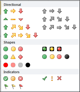
In Microsoft Excel, there are 4 different kinds of icon sets: directional, shapes, indicators and ratings. When creating your own rule, you can use any icon from any set and assign any value to it.
To create your own custom icon set, follow these steps:
- Select the range of cells where you want to apply the icons.
- Click Conditional Formatting >Icon Sets >More Rules.
- In the New Formatting Rule dialog box, select the desired icons. From the Type dropdown box, select Percentage, Number of Formula, and type the corresponding values in the Value boxes.
- Finally, click OK.
For this example, we’ve created a custom three-flags icon set, where:
- Green flag marks household spendings greater than or equal to $100.
- Yellow flag is assigned to numbers less than $100 and greater than or equal to $30.
- Green flag is used for values less than $30.
How to set conditions based on another cell value
Instead of «hardcoding» the criteria in a rule, you can input each condition in a separate cell, and then refer to those cells. The key benefit of this approach is that you can easily modify the conditions by changing the values in the referenced cells without editing the rule.
For example, we’ve entered the two main conditions in cells G2 and G3 and configured the rule in this way:
- For Type, pick Formula.
- For the Value box, enter the cell address preceded with the equality sign. To get it done automatically by Excel, just place the cursor in the box and click the cell on the sheet.
Excel conditional formatting icon sets formula
To have the conditions calculated automatically by Excel, you can express them using a formula.
To apply conditional formatting with formula-driven icons, start creating a custom icon set as described above. In the New Formatting Rule dialog box, from the Type dropdown box, select Formula, and insert your formula in the Value box.
For this example, the following formulas are used:
- Green flag is assigned to numbers greater than or equal to an average + 10:
=AVERAGE($B$2:$B$13)+10
Yellow flag is assigned to numbers less than an average + 10 and greater than or equal to an average — 20.
=AVERAGE($B$2:$B$13)-20
Note. It’s not possible to use relative references in icon set formulas.
Excel conditional format icon set to compare 2 columns
When comparing two columns, conditional formatting icon sets, such as colored arrows, can give you an excellent visual representation of the comparison. This can be done by using an icon set in combination with a formula that calculates the difference between the values in two columns — the percent change formula works nicely for this purpose.
Suppose you have the June and July spendings in columns B and C, respectively. To calculate how much the amount has changed between the two months, the formula in D2 copied down is:
Now, we want to display:
- An up arrow if the percent change is a positive number (value in column C is greater than in column B).
- A down arrow if the difference is a negative number (value in column C is less than in column B).
- A horizontal arrow if the percent change is zero (columns B and C are equal).
To accomplish this, you create a custom icon set rule with these settings:
- A green up arrow when Value is > 0.
- A yellow right arrow when Value is =0, which limits the choice to zeros.
- A red down arrow when Value is
To show only the icons without percentages, tick the Show Icon Only checkbox.
How to apply Excel icon sets based on another cell
A common opinion is that Excel conditional formatting icon sets can only be used to format cells based on their own values. Technically, that is true. However, you can emulate the conditional format icon set based on a value in another cell.
Suppose you have payment dates in column D. Your goal is to place a green flag in column A when a certain bill is paid, i.e. there is a date in the corresponding cell in column D. If a cell in column D is blank, a red flag should be inserted.
To accomplish the task, these are the steps to perform:
- Start with adding the below formula to A2, and then copy it down the column:
The formula says to return 3 if D2 is not empty, otherwise 1.
- Green flag when the number is >=3.
- Yellow flag when the number is >2. As you remember, we do not really want a yellow flag anywhere, so we set a condition that will never be satisfied, i.e. a value less than 3 and greater than 2.
- In the Type dropdown box, pick Number for both icons.
- Select the Icon Set Only checkbox to hide the numbers and only show the icons.
The result is exactly as we were looking for: the green flag if a cell in column D contains anything in it and the red flag if the cell is empty.
Excel conditional formatting icon sets based on text
By default, Excel icon sets are designed for formatting numbers, not text. But with just a little creativity, you can assign different icons to specific text values, so you can see at a glance what text is in this or that cell.
Suppose you’ve added the Note column to your household spendings table and want to apply certain icons based on the text labels in that column. The task requires some preparatory work such as:
- Make a summary table (F2:G4) numbering each note. The idea is to use a positive, negative, and zero number here.
- Add one more column to the original table named Icon (it’s where the icons are going to be placed).
- Populated the new column with a VLOOKUP formula that looks up the notes and returns matching numbers from the summary table:
=VLOOKUP(C2, $F$2:$G$4, 2, FALSE)
Now, it’s time to add icons to our text notes:
- Select the range D2:D13 and click Conditional Formatting>Icon Sets >More Rules.
- Choose the icon style you want and configure the rule as in the image below:
Where «Good» is the display value for positive numbers, «Exorbitant» for negative numbers, and «Acceptable» for 0. Please be sure to correctly replace those values with your text.
This is very close to the desired result, isn’t it?
Note. In this example, we’ve used a 3-icon set. Applying 5-icon sets based on text is also possible but requires more manipulations.
How to show only some items of the icon set
Excel’s inbuilt 3-icon and 5-icon sets look nice, but sometimes you may find them a bit inundated with graphics. The solution is to keep only those icons that draw attention to the most important items, say, best performing or worst performing.
For example, when highlighting the spendings with different icons, you may want to show only those that mark the amounts higher than average. Let’s see how you can do this:
- Create a new conditional formatting rule by clicking Conditional formatting > New Rule > Format only cells that contain. Choose to format cells with values less than average, which is returned by the below formula. Click OK without setting any format.
As a result, the icons are only shown for the amounts that are greater than average in the applied range:
How to add custom icon set to Excel
Excel’s built-in sets have a limited collection of icons and, unfortunately, there is no way to add custom icons to the collection. Luckily, there is a workaround that allows you to mimic conditional formatting with custom icons.
To emulate Excel conditional formatting with a custom icon set, these are the steps to follow:
- Create a reference table outlining your conditions as shown in the screenshot below.
- In the reference table, insert the desired icons. For this, clicking the Insert tab >Symbols group >Symbol button. In the Symbol dialog box, select the Windings font, pick the symbol you want, and click Insert.
- Next to each icon, type its character code, which is displayed near the bottom of the Symbol dialog box.
For the column where the icons should appear, set the Wingdings font, and then enter the nested IF formula like this one:
=IF(B2>=90, CHAR(76), IF(B2>=30, CHAR(75), CHAR(74)))
With cell references, it takes this shape:
=IF(B2>=$H$2, CHAR($F$2), IF(B2>=$H$3, CHAR($F$3), CHAR($F$4)))
Copy the formula down the column, and you will get this result:
Black and white icons appear rather dull, but you can give them a better look by coloring the cells. For this, you can apply the inbuilt rule (Conditional Formatting > Highlight Cells Rules > Equal To) based on the CHAR formula such as:
Now, our custom icon formatting looks nicer, right?
Method 2. Add custom icons using virtual keyboard
Adding custom icons with the help of the virtual keyboard is even easier. The steps are:
- Start by opening the virtual keyboard on the task bar. If the keyboard icon is not there, right-click on the bar, and then click Show Touch Keyboard Button.
- In your summary table, select the cell where you want to insert the icon, and then click on the icon you like.
Alternatively, you can open the emoji keyboard by pressing the Win + . shortcut (the Windows logo key and the period key together) and select the icons there.
In the Custom Icon column, enter this formula:
In this case, you need neither the character codes nor fiddling with the font type.
When added to Excel desktop, the icons are black and white:
In Excel Online, colored icons look a lot more beautiful:
This is how to use icon sets in Excel. Upon a closer look, they are capable of a lot more than just a few preset formats, right? If you are curious to learn other conditional formatting types, the tutorials linked below may come in handy.
Источник
In Excel 2007 and Excel 2010, you can use icon sets in conditional formatting. There are built-in icon sets, and in Excel 2010 you can Customize Excel Conditional Formatting Icons, to some extent. Here’s how to do that, and a workaround to create icons on the worksheet instead.
Built-in Conditional Formatting Icons
There is a good selection of built-in Excel Conditional Formatting Icon sets. For example, use Red, Yellow and Green stoplight icons, to highlight the good, average, and poor results in your sales data.
Limit the Colours
Rob emailed me recently, to ask how to limit the conditional formatting icons to 2 colours only, instead of the 3 or 4 default icon colours.
I am only interested in using 1 or 2 icons (a red X for “Off” and a Green light for “On” – not interested in the Yellow light). I want these icons to be triggered by a boolean (TRUE/FALSE) in another cell.
Create Your Own Icon Set in Excel 2010
Fortunately, if you’re using Excel 2010, you aren’t limited to the default icon sets – you can create your own icon sets , by mixing and matching from the available icons. (You can’t create your own icons, unfortunately, or change the look of the built-in icons.)
To create the icon set that Rob wants, I selected cells B2:B5, and set the following Formatting Rule.
- The Show Icon Only option is checked
- Green Circle icon when the value is greater than or equal to 1 (Number)
- Red X icon when the value is less than 1 and greater than or equal to 0 (Number)
- No Cell Icon when the value is less than 0

How It Works
In cell B2 there is a formula to multiply the value in cell A2 by 1:
=A2*1
That formula is copied down to cell B5.
- If the result in column A is TRUE, the formula result in column B is 1, and a green circle shows.
- If the result in column A is FALSE, the formula result in column B is 0, and a red X shows.

Create Your Own Icon Set in Excel 2007 and Earlier
For earlier versions of Excel, where you can’t customize the icon sets, or in Excel version where icon sets don’t exist, there is a workaround. You can use the WingDing font, combined with conditional formatting, to show coloured symbols in the cell.
There are detailed instructions in this article: Conditional Formatting Icons in Excel 2003

_______________