
The IF function allows you to make a logical comparison between a value and what you expect by testing for a condition and returning a result if that condition is True or False.
-
=IF(Something is True, then do something, otherwise do something else)
But what if you need to test multiple conditions, where let’s say all conditions need to be True or False (AND), or only one condition needs to be True or False (OR), or if you want to check if a condition does NOT meet your criteria? All 3 functions can be used on their own, but it’s much more common to see them paired with IF functions.
Use the IF function along with AND, OR and NOT to perform multiple evaluations if conditions are True or False.
Syntax
-
IF(AND()) — IF(AND(logical1, [logical2], …), value_if_true, [value_if_false]))
-
IF(OR()) — IF(OR(logical1, [logical2], …), value_if_true, [value_if_false]))
-
IF(NOT()) — IF(NOT(logical1), value_if_true, [value_if_false]))
|
Argument name |
Description |
|
|
logical_test (required) |
The condition you want to test. |
|
|
value_if_true (required) |
The value that you want returned if the result of logical_test is TRUE. |
|
|
value_if_false (optional) |
The value that you want returned if the result of logical_test is FALSE. |
|
Here are overviews of how to structure AND, OR and NOT functions individually. When you combine each one of them with an IF statement, they read like this:
-
AND – =IF(AND(Something is True, Something else is True), Value if True, Value if False)
-
OR – =IF(OR(Something is True, Something else is True), Value if True, Value if False)
-
NOT – =IF(NOT(Something is True), Value if True, Value if False)
Examples
Following are examples of some common nested IF(AND()), IF(OR()) and IF(NOT()) statements. The AND and OR functions can support up to 255 individual conditions, but it’s not good practice to use more than a few because complex, nested formulas can get very difficult to build, test and maintain. The NOT function only takes one condition.

Here are the formulas spelled out according to their logic:
|
Formula |
Description |
|---|---|
|
=IF(AND(A2>0,B2<100),TRUE, FALSE) |
IF A2 (25) is greater than 0, AND B2 (75) is less than 100, then return TRUE, otherwise return FALSE. In this case both conditions are true, so TRUE is returned. |
|
=IF(AND(A3=»Red»,B3=»Green»),TRUE,FALSE) |
If A3 (“Blue”) = “Red”, AND B3 (“Green”) equals “Green” then return TRUE, otherwise return FALSE. In this case only the first condition is true, so FALSE is returned. |
|
=IF(OR(A4>0,B4<50),TRUE, FALSE) |
IF A4 (25) is greater than 0, OR B4 (75) is less than 50, then return TRUE, otherwise return FALSE. In this case, only the first condition is TRUE, but since OR only requires one argument to be true the formula returns TRUE. |
|
=IF(OR(A5=»Red»,B5=»Green»),TRUE,FALSE) |
IF A5 (“Blue”) equals “Red”, OR B5 (“Green”) equals “Green” then return TRUE, otherwise return FALSE. In this case, the second argument is True, so the formula returns TRUE. |
|
=IF(NOT(A6>50),TRUE,FALSE) |
IF A6 (25) is NOT greater than 50, then return TRUE, otherwise return FALSE. In this case 25 is not greater than 50, so the formula returns TRUE. |
|
=IF(NOT(A7=»Red»),TRUE,FALSE) |
IF A7 (“Blue”) is NOT equal to “Red”, then return TRUE, otherwise return FALSE. |
Note that all of the examples have a closing parenthesis after their respective conditions are entered. The remaining True/False arguments are then left as part of the outer IF statement. You can also substitute Text or Numeric values for the TRUE/FALSE values to be returned in the examples.
Here are some examples of using AND, OR and NOT to evaluate dates.

Here are the formulas spelled out according to their logic:
|
Formula |
Description |
|---|---|
|
=IF(A2>B2,TRUE,FALSE) |
IF A2 is greater than B2, return TRUE, otherwise return FALSE. 03/12/14 is greater than 01/01/14, so the formula returns TRUE. |
|
=IF(AND(A3>B2,A3<C2),TRUE,FALSE) |
IF A3 is greater than B2 AND A3 is less than C2, return TRUE, otherwise return FALSE. In this case both arguments are true, so the formula returns TRUE. |
|
=IF(OR(A4>B2,A4<B2+60),TRUE,FALSE) |
IF A4 is greater than B2 OR A4 is less than B2 + 60, return TRUE, otherwise return FALSE. In this case the first argument is true, but the second is false. Since OR only needs one of the arguments to be true, the formula returns TRUE. If you use the Evaluate Formula Wizard from the Formula tab you’ll see how Excel evaluates the formula. |
|
=IF(NOT(A5>B2),TRUE,FALSE) |
IF A5 is not greater than B2, then return TRUE, otherwise return FALSE. In this case, A5 is greater than B2, so the formula returns FALSE. |

Using AND, OR and NOT with Conditional Formatting
You can also use AND, OR and NOT to set Conditional Formatting criteria with the formula option. When you do this you can omit the IF function and use AND, OR and NOT on their own.
From the Home tab, click Conditional Formatting > New Rule. Next, select the “Use a formula to determine which cells to format” option, enter your formula and apply the format of your choice.

Using the earlier Dates example, here is what the formulas would be.

|
Formula |
Description |
|---|---|
|
=A2>B2 |
If A2 is greater than B2, format the cell, otherwise do nothing. |
|
=AND(A3>B2,A3<C2) |
If A3 is greater than B2 AND A3 is less than C2, format the cell, otherwise do nothing. |
|
=OR(A4>B2,A4<B2+60) |
If A4 is greater than B2 OR A4 is less than B2 plus 60 (days), then format the cell, otherwise do nothing. |
|
=NOT(A5>B2) |
If A5 is NOT greater than B2, format the cell, otherwise do nothing. In this case A5 is greater than B2, so the result will return FALSE. If you were to change the formula to =NOT(B2>A5) it would return TRUE and the cell would be formatted. |
Note: A common error is to enter your formula into Conditional Formatting without the equals sign (=). If you do this you’ll see that the Conditional Formatting dialog will add the equals sign and quotes to the formula — =»OR(A4>B2,A4<B2+60)», so you’ll need to remove the quotes before the formula will respond properly.
Need more help?

See also
You can always ask an expert in the Excel Tech Community or get support in the Answers community.
Learn how to use nested functions in a formula
IF function
AND function
OR function
NOT function
Overview of formulas in Excel
How to avoid broken formulas
Detect errors in formulas
Keyboard shortcuts in Excel
Logical functions (reference)
Excel functions (alphabetical)
Excel functions (by category)
Conditional formatting is a fantastic way to quickly visualize data in a spreadsheet. With conditional formatting, you can do things like highlight dates in the next 30 days, flag data entry problems, highlight rows that contain top customers, show duplicates, and more.
Excel ships with a large number of «presets» that make it easy to create new rules without formulas. However, you can also create rules with your own custom formulas. By using your own formula, you take over the condition that triggers a rule and can apply exactly the logic you need. Formulas give you maximum power and flexibility.
For example, using the «Equal to» preset, it’s easy to highlight cells equal to «apple».
But what if you want to highlight cells equal to «apple» or «kiwi» or «lime»? Sure, you can create a rule for each value, but that’s a lot of trouble. Instead, you can simply use one rule based on a formula with the OR function:

Here’s the result of the rule applied to the range B4:F8 in this spreadsheet:

Here’s the exact formula used:
=OR(B4="apple",B4="kiwi",B4="lime")
Quick start
You can create a formula-based conditional formatting rule in four easy steps:
1. Select the cells you want to format.

2. Create a conditional formatting rule, and select the Formula option

3. Enter a formula that returns TRUE or FALSE.

4. Set formatting options and save the rule.

The ISODD function only returns TRUE for odd numbers, triggering the rule:

Video: How to apply conditional formatting with a formula
Formula logic
Formulas that apply conditional formatting must return TRUE or FALSE, or numeric equivalents. Here are some examples:
=ISODD(A1)
=ISNUMBER(A1)
=A1>100
=AND(A1>100,B1<50)
=OR(F1="MN",F1="WI")
The above formulas all return TRUE or FALSE, so they work perfectly as a trigger for conditional formatting.
When conditional formatting is applied to a range of cells, enter cell references with respect to the first row and column in the selection (i.e. the upper-left cell). The trick to understanding how conditional formatting formulas work is to visualize the same formula being applied to each cell in the selection, with cell references updated as usual. Imagine that you entered the formula in the upper-left cell of the selection, and then copied the formula across the entire selection. If you struggle with this, see the section on Dummy Formulas below.
Formula Examples
Below are examples of custom formulas you can use to apply conditional formatting. Some of these examples can be created using Excel’s built-in presets for highlighting cells, but custom formulas can go far beyond presets, as you can see below.
Highlight orders from Texas
To highlight rows that represent orders from Texas (abbreviated TX), use a formula that locks the reference to column F:
=$F5="TX"

For more details, see this article: Highlight rows with conditional formatting.
Video: How to highlight rows with conditional formatting
Highlight dates in the next 30 days
To highlight dates occurring in the next 30 days, we need a formula that (1) makes sure dates are in the future and (2) makes sure dates are 30 days or less from today. One way to do this is to use the AND function together with the NOW function like this:
=AND(B4>NOW(),B4<=(NOW()+30))
With a current date of August 18, 2016, the conditional formatting highlights dates as follows:

The NOW function returns the current date and time. For details about how this formula, works, see this article: Highlight dates in the next N days.
Highlight column differences
Given two columns that contain similar information, you can use conditional formatting to spot subtle differences. The formula used to trigger the formatting below is:
=$B4<>$C4

See also: a version of this formula that uses the EXACT function to do a case-sensitive comparison.
Highlight missing values
To highlight values in one list that are missing from another, you can use a formula based on the COUNTIF function:
=COUNTIF(list,B5)=0

This formula simply checks each value in List A against values in the named range «list» (D5:D10). When the count is zero, the formula returns TRUE and triggers the rule, which highlights values in List A that are missing from List B.
Video: How to find missing values with COUNTIF
Highlight properties with 3+ bedrooms under $350k
To find properties in this list that have at least 3 bedrooms but are less than $300,000, you can use a formula based on the AND function:
=AND($C5<350000,$D5>=3)
The dollar signs ($) lock the reference to columns C and D, and the AND function is used to make sure both conditions are TRUE. In rows where the AND function returns TRUE, the conditional formatting is applied:

Highlight top values (dynamic example)
Although Excel has presets for «top values», this example shows how to do the same thing with a formula, and how formulas can be more flexible. By using a formula, we can make the worksheet interactive — when the value in F2 is updated, the rule instantly responds and highlights new values.

The formula used for this rule is:
=B4>=LARGE(data,input)
Where «data» is the named range B4:G11, and «input» is the named range F2. This page has details and a full explanation.
Gantt charts
Believe it or not, you can even use formulas to create simple Gantt charts with conditional formatting like this:

This worksheet uses two rules, one for the bars, and one for the weekend shading:
=AND(D$4>=$B5,D$4<=$C5) // bars
=WEEKDAY(D$4,2)>5 // weekends
This article explains the formula for bars, and this article explains the formula for weekend shading.
Simple search box
One cool trick you can do with conditional formatting is to build a simple search box. In this example, a rule highlights cells in column B that contain text typed in cell F2:

The formula used is:
=ISNUMBER(SEARCH($F$2,B2))
For more details and a full explanation, see:
- Article: How to highlight cells that contain specific text
- Article: How to highlight rows that contain specific text
- Video: How to build a search box to highlight data
Troubleshooting
If you can’t get your conditional formatting rules to fire correctly, there’s most likely a problem with your formula. First, make sure you started the formula with an equals sign (=). If you forget this step, Excel will silently convert your entire formula to text, rendering it useless. To fix, just remove the double quotes Excel added at either side and make sure the formula begins with equals (=).
If your formula is entered correctly but is not triggering the rule, you may have to dig a little deeper. Normally, you can use the F9 key to check results in a formula or use the Evaluate feature to step through a formula. Unfortunately, you can’t use these tools with conditional formatting formulas, but you can use a technique called «dummy formulas».
Dummy Formulas
Dummy formulas are a way to test your conditional formatting formulas directly on the worksheet, so you can see what they’re actually doing. This can be a big time-saver when you’re struggling to get cell references working correctly.
In a nutshell, you enter the same formula across a range of cells that matches the shape of your data. This lets you see the values returned by each formula, and it’s a great way to visualize and understand how formula-based conditional formatting works. For a detailed explanation, see this article.

Video: Test conditional formatting with dummy formulas
Limitations
There are some limitations that come with formula-based conditional formatting:
- You can’t apply icons, color scales, or data bars with a custom formula. You are limited to standard cell formatting, including number formats, font, fill color and border options.
- You can’t use certain formula constructs like unions, intersections, or array constants for conditional formatting criteria.
- You can’t reference other workbooks in a conditional formatting formula.
You can sometimes work around #2 and #3. You may be able to move the logic of the formula into a cell in the worksheet, then refer to that cell in the formula instead. If you are trying to use an array constant, try created a named range instead.
More CF formula resources
- More than 30 conditional formatting formulas examples
- Video training with practice worksheets
Conditional Formatting is an excellent way to visualize the data based on certain criteria. OR function in the Conditional Formatting highlights the data in the table if at least one of the defined conditions is met. This step by step tutorial will assist all levels of Excel users in creating a Conditional Formatting OR formula rule.
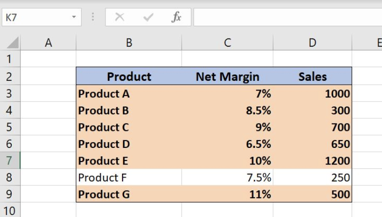
Figure 1. Final result
Syntax of the OR formula
=OR(logical1,[logical2], …)
The parameters of the OR function are:
- Logical1, logical2 – the conditions that we want to test
The output of the formula is value TRUE if just one condition is met. If neither of the conditions is met formula result will be FALSE
Highlight cell values using OR function
To mark the rows in the table based on the certain criteria we can use formula rules in the Conditional Formatting. In our example, we want to emphasize the rows in the table where Net Margin is over 8% or Sales are over 600. For this purpose, we will use OR function since it’s enough that only one condition is met.
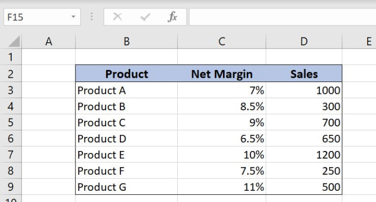 Figure 2. Highlight rows where Net Margin is over 8% or Sales is over 600
Create an OR formula rule in the Conditional Formatting
To create a Conditional Formatting rule based on the formula we should follow the steps below:
- Select the cell, cell range or table in Excel where we what to apply the Conditional Formatting
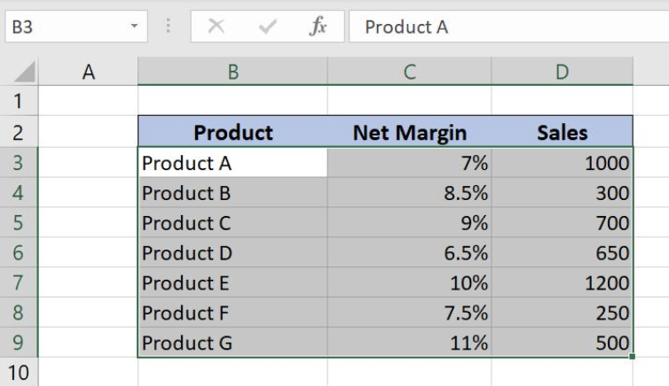 Figure 3. Select a cell range for the Conditional Formatting
- Find Conditional Formatting button tab and choose New Rule
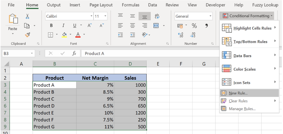 Figure 4. Create a new rule in the Conditional Formatting
- Choose Use a formula to determine which cells to format
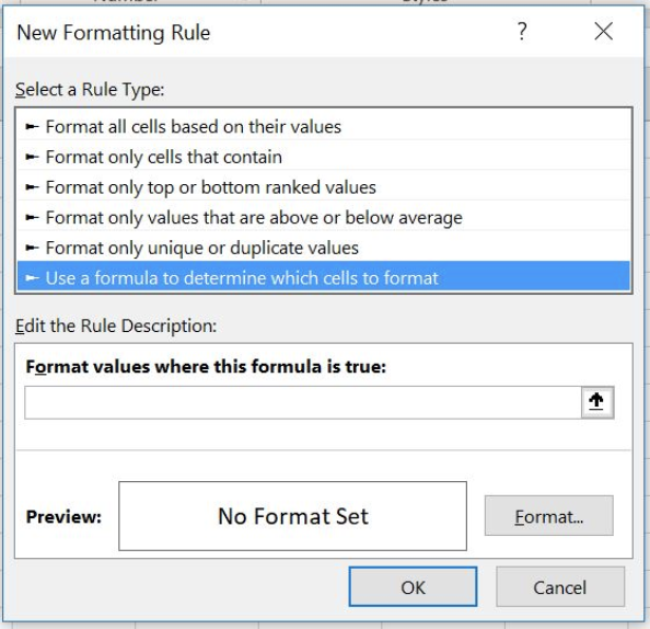 Figure 5. Create a formula rule in Conditional Formatting
- Enter formula rule under the section Format values where this formula is true
=OR($C3>8%,$D3>600)
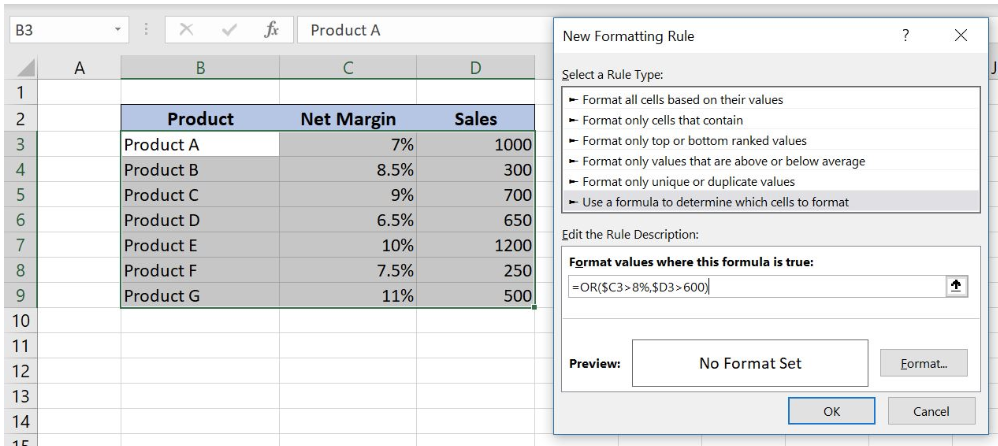 Figure 6. OR function in Conditional Formatting
The formula above highlights the rows in the example table where Net Margin is over 8% or Sales is over 600. OR function checks if at least one condition is met and returns the value TRUE. This value triggers the Conditional Formatting rule.
In our OR formula example there are two logical tests:
- Logical1 is $C3>8% – checks if Net Margin is over 8%
- Logical2 is $D3>600 – examines if Sales is over 600
- Under the Format tab, we can define the visual appearance of the cells if the OR formula output is TRUE
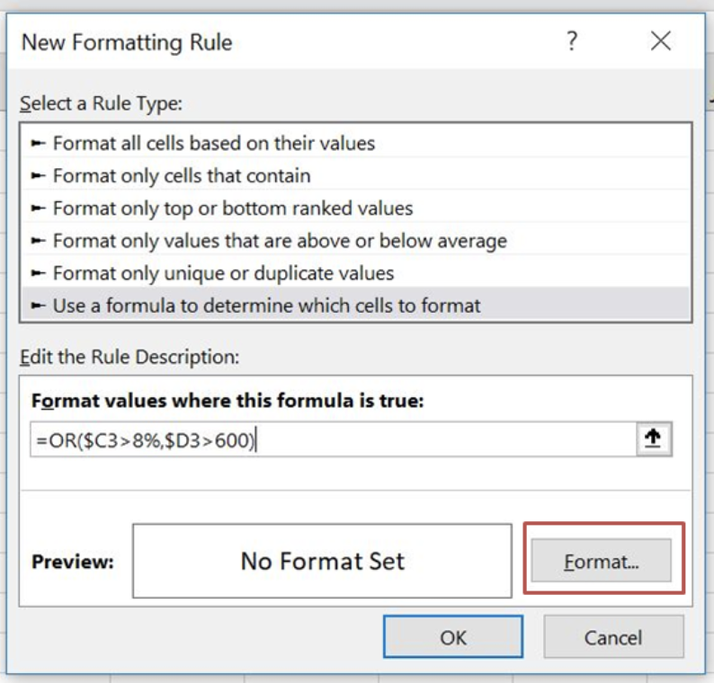 Figure 7. Create a custom format in Conditional Formatting
- In Fill tab choose the background color (here you can also choose pattern style and color)
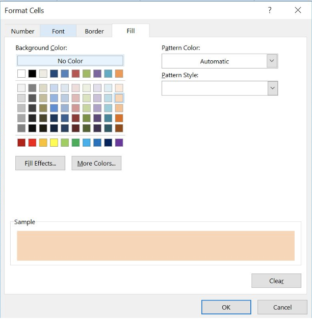 Figure 8. Define a Background Color of the cells
- In the Font tab we can define font style and Bold cell text
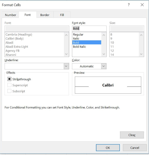 Figure 9. Choose a Font style of the cells
- After choosing the format in section Preview we can see how Conditional Formatting cells will look like if the rule is met
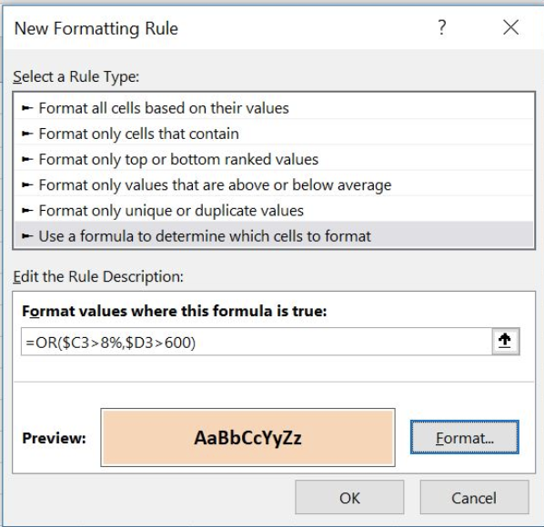 Figure 10. Conditional Formatting rule Preview
- Rows in the table are highlighted whenever the Net Margin is over 8% or Sales is over 600. Product F in the table is the only product that meets neither Net Margin nor Sales condition.
Figure 11. Conditional Formatting OR formula rule- Net Margin over 8% or Sales over 600
Most of the time, the problem you will need to solve will be more complex than a simple application of a formula or function. If you want to save hours of research and frustration, try our live Excelchat service! Our Excel Experts are available 24/7 to answer any Excel question you may have. We guarantee a connection within 30 seconds and a customized solution within 20 minutes.
In this article we will learn how to color rows based on text criteria we use the “Conditional Formatting” option. This option is available in the “Home Tab” in the “Styles” group in Microsoft Excel.
Conditional Formatting in Excel is used to highlight the data on the basis of some criteria. It would be difficult to see various trends just for examining your Excel worksheet. Conditional Formatting in excel provides a way to visualize data and make worksheets easier to understand.
Excel Conditional Formatting allows you to apply formatting basis on the cell values such as colors, icons and data bars. For this, we will create a rule in excel Conditional Formatting based on cell value
How to write an if statement in excel?
IF function is used for logic_test and returns value on the basis of the result of the logic_test. Excel conditional formatting formula multiple conditions uses Statements like less than or equal to or greater than or equal to the value are used in IF formula
Syntax:
=IF (logical_test, [value_if_true], [value_if_false])
Let’s learn how to do conditional formatting in excel using IF function with the example.
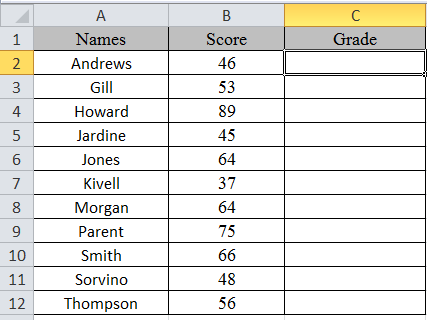
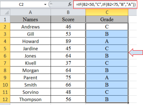
Here is a list of Names and their respective Scores.
multiple if statements excel functions are used here. So, there are 3 results based on the condition. if then statements in excel is used via excel conditional formatting formula
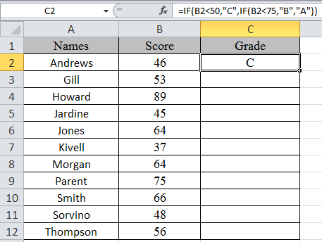
Write the formula in C2 cell.
Formula
=IF(B2<50,»C»,IF(B2<75,»B»,»A»))
Explanation:
IF function only returns 2 results, one [value_if_True] and Second [value-if_False]
First IF function checks, if the score is less than 50, would get C grade, The Second IF function tests if the score is less than 75 would get B grade and the rest A grade.
Copy the formula in other cells, select the cells taking the first cell where the formula is already applied, use shortcut key Ctrl + D
Now we will apply conditional formatting to it.
Select Home >Conditional Formatting > New Rule.
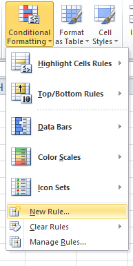
A dialog box appears
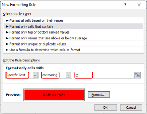
Select Format only cells that contain > Specific text in option list and write C as text to be formatted.
Fill Format with Red colour and click OK.
Now select the colour Yellow and Green for A and B respectively as done above for C.
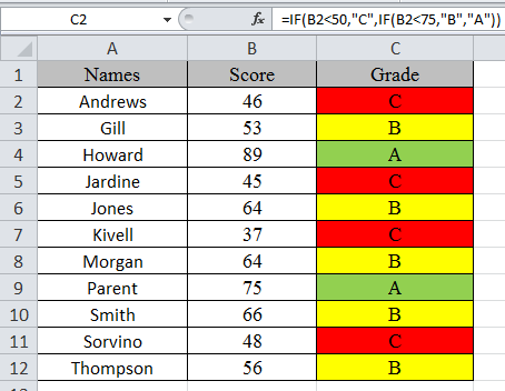
In this article, we used IF function and Conditional formatting tool to get highlighted grade.
As you can see excel change cell color based on value of another cell using IF function and Conditional formatting tool
Hope you learned how to use conditional formatting in Excel using IF function. Explore more conditional formulas in excel here. You can perform Conditional Formatting in Excel 2016, 2013 and 2010. If you have any unresolved query regarding this article, please do mention below. We will help you.
Related Articles:
How to use the Conditional formatting based on another cell value in Excel
How to use the Conditional Formatting using VBA in Microsoft Excel
How to use the Highlight cells that contain specific text in Excel
How to Sum Multiple Columns with Condition in Excel
Popular Articles:
50 Excel Shortcut to Increase Your Productivity
How to use the VLOOKUP Function in Excel
How to use the COUNTIF function in Excel 2016
How to use the SUMIF Function in Excel
The best part of conditional formatting is you can use formulas in it. And, it has a very simple sense to work with formulas.
Your formula should be a logical formula and the result should be TRUE or FALSE. If the formula returns TRUE, you’ll get the formatting, and if FALSE then nothing. The point is, by using formulas you can make the best out of conditional formatting.
Yes, that’s right. In the below example, we have used a formula in CF to check whether the value in the cell is smaller than 1000 or not.

And if that value is smaller than 1000 it will apply the formatting which we have specified, otherwise not. So today in this post, I’d like to share with you simple steps to apply conditional formatting using a formula. And some of the useful examples that you can use in your daily work.
Steps to Apply Conditional Formatting with Formulas
The steps to apply CF with formulas are quite simple:
- Select the range to apply Conditional Formatting.
- Add a formula to text a condition.
- Specify a format to apply when the condition is met.

To learn this in a proper way make sure to download this sample file from here and follow the below-detailed steps.
- First of all, select the range where you want to apply conditional formatting.

- After that, go to Home Tab ➜ Styles ➜ Conditional Formatting ➜ New Rule ➜ Use a formula to determine which cell to format.

- Now, in the “Format values where formula is true” enter the below formula.
=E5<1000

- The next thing is to specify the format to apply and for this, click on the format button and select the format.

- In the end, click OK.
While entering a formula in the CF dialog box you can’t see its result or whether that formula is valid or not. So, the best practice is to check that formula before using it in CF by entering it in a cell.
1. Use a Formula that is Based on Another Cell
Yes, you can apply conditional formatting based on another cell’s value. If you look at the below example, we have added a simple formula that is based on another cell. And if the value of that linked cell meets the condition specified, you’ll get conditional formatting.

When achievement will be below 75%, it will highlight in red color.

2. Conditional Formatting using IF
Whenever I think about conditions, the first thing that comes to my mind is using the IF function. And the best part of this function is, that it fits perfectly in conditional formatting. Let me show you an example:

Here, we have used the IF to create a condition and the condition is when the count of “Done” in range B3:B9 is equal to the count of tasks in the range A3:A9, then the final status will appear.
2. Conditional Formatting with Multiple Conditions
You can create multiple checks in conditions to apply to the format. Once all the conditions or one of the conditions will meet, conditional formatting will apply to the cell. Look at the below example where we have used the average temperature of my town.
And we have used a simply combined IF-AND to highlight the months when the temperature is pretty pleasant. Months where the temperature is between 15 Celsius to 35 Celsius, will get colored.
Just like this, you can also use if with or function.
4. Highlight Alternate Rows with Conditional Formatting
To highlight every alternate row you can use the following formula n CF.
=INT(MOD(ROW(),2))
By using this formula, every row whose number is odd will be highlighted. And, if you want to do vice versa you can use the following formula.

=INT(MOD(ROW()+1,2))
The same kind of formula can use for columns (odd and even) as well.
=INT(MOD(COLUMN(),2))
And for even columns.
=INT(MOD(COLUMN()+1,2))
5. Highlight Cells with Errors using CF
Now let’s come to another example where we will check whether a cell contains an error or not. What we need to do is just insert a formula in conditional formatting that can check the condition and return the result in TRUE or FALSE. You can even verify cells for numbers, text, or some specific values as well.

6. Create a Checklist with Conditional Formatting
Now let’s add some creativity to intelligence. You have already learned how to use a formula that is based on another cell. Here we have linked a checkbox with the B1 cell and further linked the B1 with the formula used in conditional formatting for cell A1.

Now, if you tick mark the checkbox, the value of cell B1 will turn into TRUE and cell A1 gets it conditional formatting [strikethrough].
Points to Remember
- Your formula should be a logical formula, which leads to a result as TRUE or FALSE.
- Try not to overload your data with conditional formatting.
- Always use relative and absolute references in a proper sense.
Sample File
Download this sample file from here to learn more.
More Tutorials
- AUTO FORMAT Option in Excel
- Apply Accounting Number Format in Excel
- Apply Background Color to a Cell or the Entire Sheet in Excel
- Print Excel Gridlines
- Add Page Number in Excel
- Apply Comma Style in Excel
- Apply Strikethrough in Excel
- Highlight Blank Cells in Excel
- Make Negative Numbers Red in Excel
- Cell Style (Title, Calculation, Total, Headings…) in Excel
- Change Date Format in Excel
- Highlight Alternate Rows in Excel with Color Shade
- Use Icon Sets in Excel (Conditional Formatting)
- Add Border in Excel
- Change Border Color in Excel
- Clear Formatting in Excel
- Copy Formatting in Excel
- Best Fonts for Microsoft Excel
- Hide Zero Values in Excel
⇠ Back to Advanced Excel Tutorials