
Example
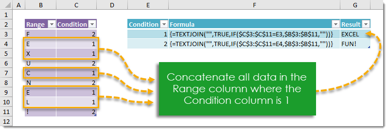
{=TEXTJOIN("",TRUE,IF($C$3:$C$11=E3,$B$3:$B$11,""))}
![]()
Generic Formula
{=TEXTJOIN(Delimiter,TRUE,IF(ConditionRange=Condition,Range,""))}
Note: This is an array formula. Do not type out the {} brackets. Hold Ctrl + Shift then press Enter while in Edit Mode to create an array formula. For Mac, use ⌘ + Shift + Return.
- Range – This is range of values which we want to concatenate together.
- Delimiter – This is the delimiter value which we want to use to separate values by in our concatenation. Use empty quotes if we don’t want to use a delimiter.
- ConditionRange – This is the range of values which we will use to test whether or not to concatenate an item from our Range.
- Condition – This is the condition to test.
What It Does
This formula will conditionally concatenate a range based on a criteria in another range.
How It Works
IF(ConditionRange=Condition,Range,””) will create an array containing data from the Range when it meets the given condition. In our example this will create the following array.
{"";"E";"X";"";"C";"";"E";"L";""}
TEXTJOIN(Delimiter,TRUE,Array) will concatenate the individual items in the Array and separating them with the chosen Delimiter. Using TRUE as the middle argument will skip any blank cells in the array. In our example TEXTJOIN(“”,TRUE,{“”;”E”;”X”;””;”C”;””;”E”;”L”;””}) results in EXCEL!
About the Author
John is a Microsoft MVP and qualified actuary with over 15 years of experience. He has worked in a variety of industries, including insurance, ad tech, and most recently Power Platform consulting. He is a keen problem solver and has a passion for using technology to make businesses more efficient.
Содержание
- Concatenate If – Excel & Google Sheets
- The CONCAT Function
- Adding Delimiters or Ignoring Empty Values
- Concatenate If – in pre-Excel 2019
- Concatenate If in Google Sheets
- How to concatenate values in multiple cells based on a condition?
- 3 Answers 3
- Write your own UDF
- Original solution.
- Excerpt from the article
- How to CONCATENATE a RANGE of Cells [Combine] in Excel
- [CONCATENATE + TRANSPOSE] to Combine Values
- How this formula works
- Combine Text using the Fill Justify Option
- TEXTJOIN Function for CONCATENATE Values
- Syntax:
- how to use it
- Combine Text with Power Query
- VBA Code to Combine Values
- In the end,
- More Formulas
- 57 thoughts on “How to CONCATENATE a RANGE of Cells [Combine] in Excel”
Concatenate If – Excel & Google Sheets
Download the example workbook
This tutorial will demonstrate how to concatenate cell values based on criteria using the CONCAT Function in Excel and Google Sheets.
The CONCAT Function
Users of Excel 2019+ have access to the CONCAT Function which is used to join multiple strings into a single string.
- Our first example uses the CONCAT Function and so is not available to Excel users before Excel 2019. See a later section in this tutorial for how to replicate this example in older versions of Excel.
- Google Sheets users also have access to the CONCAT Function, but unlike in Excel, it only allows two values or cell references to be joined together and does not allow inputs of cell ranges. See a later section on how this example can be achieved in Google Sheets by using the TEXTJOIN Function instead.
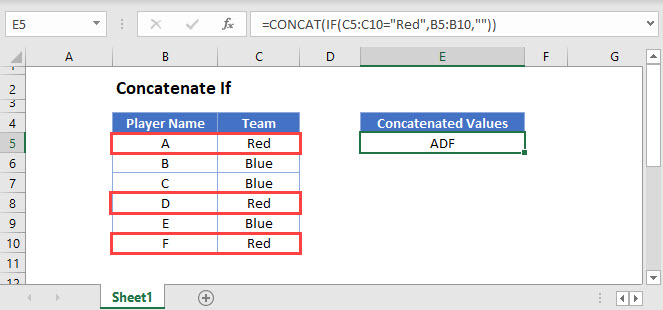
This example will use the CONCAT and IF Functions in an array formula to create a text string of Player Names which relate to a Team value of Red
Users of Excel 2019 will need to enter this formula as an array function by pressing CTRL + SHIFT + ENTER. Users of later versions of Excel do not need to follow this step.
To explain what this formula is doing, lets break it down into steps:
This is our final formula:
First, Excel reads the range values into the formula:
Next the list of Team names is compared to the value Red:
The IF Function replaces TRUE values with the Player Name, and FALSE values with “”
The CONCAT Function then combines all of the array values into one text string:
Adding Delimiters or Ignoring Empty Values
If it is required to add delimiting values or text between each value, or for the function to ignore empty cell values, The TEXTJOIN Function can be used instead if you need to add delimiters
Read our TEXTJOIN If article to learn more.
Concatenate If – in pre-Excel 2019
As the CONCAT and TEXTJOIN Functions are not available before the Excel 2019 version, we need to solve this problem in a different way. The CONCATENATE Function is available but does not take ranges of cells as inputs or allow array operations and so we are required to use a helper column with an IF Function instead.
This next example shows how to use a helper column to create a text string of Player Names which relate to a Team value of Red:
The first step in this example is to use an IF Function to replicate the condition of Team = Red:
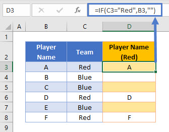
Next, we can create a column that builds up a list of these values into one cell by also referencing the cell below it:
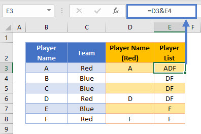
This formula uses the & character to join two values together. Note that the CONCATENATE Function could be used to create exactly the same result, but the & method is often preferred as it is shorter and makes it clearer what action the formula is performing.
These two helper columns can then be combined into one formula:
A summary cell can then reference the first value in the Player List helper column:
Concatenate If in Google Sheets
Google Sheets users should use the TEXTJOIN Function to concatenate values based on a condition.
This example will use the TEXTJOIN and IF Functions to create a text string of Player Names which relate to a Team value of Red
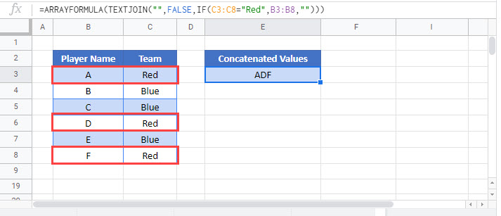
As this formula requires array inputs for the cell ranges, the ARRAYFORMULA Function should be added to the formula by pressing CTRL + SHIFT + ENTER.
Источник
How to concatenate values in multiple cells based on a condition?
I have a need to search a row of cells, and for every cell that contains a specific value, return the value from the cell above.
For example, consider the following
So I want to insert a formula into cells F2, F3 and F4 which will give the following results
Can this be done?
3 Answers 3
I have found a simple, scalable solution that uses an array formula to concatenate multiple cells that satisfy a certain condition.
Applied to your example, paste into cell F2:
and hit ctrl+shift+enter to enter as an array formula, and copy over cells F3—F4.
The reason why this works is left as an exercise to the reader. It’s fairly clear, but I prefer «magic».
I hope this helps anyone with a similar problem.

Write your own UDF
Original solution.
Excerpt from the article
- Open VBA Editor by clicking Visual Basic on Developer tab or using Alt + F11 combination
- Create new module by right clicking Microsoft Excel Objects in the top left corner and choosing Insert->Module from the context menu.
- Insert the following code
Later on you can use it, if you enable macro in your workbook.
In your specific example write the following formula into F2 cell and copy over needed range.
In F2 copy-paste this formula:
and drag down against the column.
The above code has been rewritten 5 times and the column name has been changed. It checks whether the cell in the current row has a ‘YES’. If it does then it’ll enter the header of the column which is ‘A$1’ . Notice that $1 is absolute reference to the first row i.e. the header.
In the end, I have encapsulated all the five IF statements using CONCATENATE statement.
Источник
How to CONCATENATE a RANGE of Cells [Combine] in Excel
Combining values with CONCATENATE is the best way, but with this function, it’s not possible to refer to an entire range.
You need to select all the cells of a range one by one, and if you try to refer to an entire range, it will return the text from the first cell.
In this situation, you do need a method where you can refer to an entire range of cells to combine them in a single cell.
So today in this post, I’d like to share with you 5 different ways to combine text from a range into a single cell.
[CONCATENATE + TRANSPOSE] to Combine Values
The best way to combine text from different cells into one cell is by using the transpose function with concatenating function .
Look at the below range of cells where you have a text but every word is in a different cell and you want to get it all in one cell.
Below are the steps you need to follow to combine values from this range of cells into one cell.
- In the B8 (edit the cell using F2), insert the following formula, and do not press enter.
- =CONCATENATE(TRANSPOSE(A1:A5)&” “)
- Now, select the entire inside portion of the concatenate function and press F9. It will convert it into an array.
- After that, remove the curly brackets from the start and the end of the array.
- In the end, hit enter.
![]()
How this formula works
In this formula, you have used TRANSPOSE and space in the CONCATENATE. When you convert that reference into hard values it returns an array.
In this array, you have the text from each cell and a space between them and when you hit enter, it combines all of them.
Combine Text using the Fill Justify Option
Fill justify is one of the unused but most powerful tools in Excel. And, whenever you need to combine text from different cells you can use it.
The best thing is, t hat you need a single click to merge text . Have look at the below data and follow the steps.
- First of all, make sure to increase the width of the column where you have text.
- After that, select all the cells.
- In the end, go to Home Tab ➜ Editing ➜ Fill ➜ Justify.
This will merge text from all the cells into the first cell of the selection.
TEXTJOIN Function for CONCATENATE Values
If you are using Excel 2016 (Office 365), there is a function called “TextJoin”. It can make it easy for you to combine text from different cells into a single cell.
Syntax:
TEXTJOIN(delimiter, ignore_empty, text1, [text2], …)
- delimiter a text string to use as a delimiter.
- ignore_empty true to ignore blank cell, false to not.
- text1 text to combine.
- [text2] text to combine optional.
how to use it
To combine the below list of values you can use the formula:
Here you have used space as a delimiter, TRUE to ignore blank cells and the entire range in a single argument. In the end, hit enter and you’ll get all the text in a single cell.
Combine Text with Power Query
Power Query is a fantastic tool and I love it. Make sure to check out this (Excel Power Query Tutorial). You can also use it to combine text from a list in a single cell. Below are the steps.
- Select the range of cells and click on “From table” in data tab.

- If will edit your data into Power Query editor.
- Now from here, select the column and go to “Transform Tab”.
- From “Transform” tab, go to Table and click on “Transpose”.
- For this, select all the columns (select first column, press and hold shift key, click on the last column) and press right click and then select “Merge”.
- After that, from Merge window, select space as a separator and name the column.
- In the end, click OK and click on “Close and Load”.


Now you have a new worksheet in your workbook with all the text in a single cell. The best thing about using Power Query is you don’t need to do this setup again and again.
When you update the old list with a new value you need to refresh your query and it will add that new value to the cell.
VBA Code to Combine Values
If you want to use a macro code to combine text from different cells then I have something for you. With this code, you can combine text in no time. All you need to do is, select the range of cells where you have the text and run this code.
Make sure to specify your desired location in the code where you want to combine the text.
In the end,
There may be different situations for you where you need to concatenate a range of cells into a single cell. And that’s why we have these different methods.
All methods are easy and quick, you need to select the right method as per your need. I must say that give a try to all the methods once and tell me:
Which one is your favorite and worked for you?
Please share your views with me in the comment section. I’d love to hear from you, and please, don’t forget to share this post with your friends, I am sure they will appreciate it.
More Formulas
57 thoughts on “How to CONCATENATE a RANGE of Cells [Combine] in Excel”
Hi the VBA portion works almost exactly for what I need. I changed the separator though to be ” || “. Doing this of course yields combined numbers separated by a space, two || symbols, and another space. However, they come out as 0943 || 0957 || 0960 || 0963 || and as you can see it puts those || symbols at the end. Is there a way to not have it put the space and the two || symbols after the last number? So that when it combines them it would only be 0943 || 0957 || 0963? If the macro can do that, that would be exactly what I need it for. Would that be an edit to the VBA and what would that edit be? Please and thank you so much!
#1 is of no use, string value is fixed at moment when concat & transpose formula written.
Super helpful post RE concatenation of a range of cells in XLS; thank you!
All your solutions are excellent.
Many different methods are also taught.
Though I am very good at Excel, I learn many many things from your website.
THANKS A LOT.
God Bless.
115750-760 ,765how to convert in column with serial wise
You’re a genius. Very very help for me. Thanks a lot.
Hello,
Is it possible via formula, w/o vba nor Power Tools, to combine 2 arrays (generated by formula) into a non-array value separated by comas. Textjoin will work with only 1 array but returns the first element when there is a division of array inside the Textjoin formula. I also tried to have another cell to do the division w/o luck. If u need to know why I’m doing this, I’ll be glad to add more details.
TQ, KR!
Thank you so much for this, the formula worked perfectly – saved me ages. Thanks 🙂
Thank you for this VBA code. It works great! However, I want to add one more aspect to the code and I can’t quite figure it out.
I would like for the code to locate a cell, based on a certain text, then select everything in the list below that cell. Is that something easily doable?
Thanks for the interesting article. Unfortunately, as far as I can see, none of the methods actually does what I want.
I am writing an accounting spreadsheet, and I want a column that shows an error message if there is anything unexpected in the columns where I enter data, or in the calculation columns. At present, it is a huge long tangle of nested if statements and messages joined by “&” operators. I want to simplify this by setting up some columns, each of which detects a particular error, and generates an appropriate message if it finds it. This will make it much easier to add more error checking in future – just insert more columns in this part of the sheet.
In this scenario, the error message column (the one that is always visible) needs to be a concatenation of all the individual error columns.
The first two methods don’t work, since they use the values of the cells at the time you type the formula, while I want one that continually updates as the data – and messages – change.
The third method doesn’t work because I am using the standalone Excel 2016, which doesn’t have TEXTJOIN. This is particularly frustrating, because TEXTJOIN is exactly the function I need!
One day, I intend to add some VBA code to my spreadsheet to cover things like year end (when I have to chop off a year’s worth of data and replace it with a few lines of carried-forward values), but I have never programmed in VB (of any flavour), so this is going to be a major project. (Maybe I’ll use Python code instead.) The problem I foresee here is that code generally executes when the user clicks a button; formulae execute when you change a cell on which they depend. If I set up a VBA program to execute every time I enter data, and it computes this for every line of the spreadsheet, it introduces a huge processing overhead! And if I (or anyone else using the sheet) can remember to click a “check for errors” button, we can remember to check for errors anyway.
So this leaves Power Query. I’d never even heard of this tool before I read your article! If (as I suspect) I need to click something to refresh my query in order to check for errors, then it suffers from the same problem as VBA. But it’s worth further investigation. Thank you for bringing it to my attention.
Maybe I need to migrate to Excel 2019. Now that I have (I think) sorted out all the bugs that were introduced when I migrated from Excel 2007 to Excel 2016, that’s a possibility. (The bugs mostly concerned the changed behaviour of SUMIF when the data range and criterion range were different lengths)
In the meantime, I shall probably set up the columns I need, and concatenate them with & or CONCATENATE. I’ll just have to remember to add more arguments to the formula whenever I add more error checking columns.
This may be a bit out of date now. However, if the above VBA is adjusted, it can be used to return the concatenated strings as a normal formula, enter (something like) the following into a VBA module (Alt-F11, Insert-Module):
“Public Function RANGECAT(rng1 As Range, Optional rng2 As Range) As String
Dim r1 As Integer, c1 As Integer, r2 As Integer, c2 As Integer
Dim cel As String
cel = “”
For c1 = 1 To rng1.Columns.Count
For r1 = 1 To rng1.Rows.Count
cel = cel + rng1.Cells(r1, c1)
Next r1
Next c1
If rng2 Is Nothing Then
Else
For c2 = 1 To rng2.Columns.Count
For r2 = 1 To rng2.Rows.Count
cel = cel + rng2.Cells(r2, c2)
Next r2
Next c2
End If
RANGECAT = cel
End Function”
The “combineText = cel” returns the value found. Further ranges can be added as needed (using “Optional rng3 as range, …” and repeating the rng2 for loops).
I have 1 Query in VBA Example : Ship Mode : Instant Air
And Customer Name’s : Jeremy Lonsdale
Cindy Schnelling
Susan Vittorini
Toby Braunhardt
Ralph Arnett
Harold Engle
Helen Abelman
Guy Armstrong
Jennifer Braxton
Giulietta Baptist
And I need the result is Instant Air
Roy Skaria, Jeremy Lonsdale, Cindy Schnelling, Susan Vittorini, Toby Braunhardt, Ralph Arnett, Harold Engle, Helen Abelman, Guy Armstrong, Jennifer Braxton, Giulietta Baptist, Erica Bern, Christopher Schild, Joy Smith, Evan Minnotte, Jenna Caffey,
Like this Instant Air Would be one line remaining all are in one line with commas how it is possible can you let me know.
first of all would like to say thankful to you because few days ago I have been working on your blogs all are most important and helpful for us again thank you so much sir
Regards
Sandeep Singh
Hi Puneet, when I try to combine cells using formula Concatenate with separater “; “ it returns “” instead of “,” after I hit F9. Does it have something to do with Excel settings? I tried it at my collegue’s PC and it works as it should and we both use Excel 2010
Источник
-
— By
Sumit Bansal
In Excel, there are two ways to combine the contents of multiple cells:
- Excel CONCATENATE function (or the ampersand (&) operator)
- Excel TEXTJOIN function (new function in Excel if you have Office 365)
If you’re using Excel with Office 365 subscription, I suggest you click here to skip to the part where the TEXTJOIN function is covered. If you’re not using Office 365, keep reading.
In its basic form, CONCATENATE function can join 2 or more characters of strings.
For example:
- =CONCATENATE(“Good”,”Morning”) will give you the result as GoodMorning
- =CONCATENATE(“Good”,” “, “Morning”) will give you the result as Good Morning
- =CONCATENATE(A1&A2) will give you the result as GoodMorning (where A1 has the text ‘Good’ in it and A2 has the text ‘Morning’.
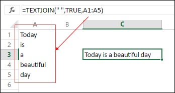
While you can enter the reference one by one within the CONCATENATE function, it would not work if you enter the reference of multiple cells at once (as shown below):
For example, in the example above, while the formula used is =CONCATENATE(A1:A5), the result only shows ‘Today’ and doesn’t combine all the cells.
In this tutorial, I will show you how to combine multiple cells by using the CONCATENATE function.
Note: If you’re using Excel 2016, you can use the TEXTJOIN function that is built to combine multiple cells using a delimiter.
CONCATENATE Excel Range (Without any Separator)

Here are the steps to concatenate an Excel range without any separator (as shown in the pic):
- Select the cell where you need the result.
- Go to formula bar and enter =TRANSPOSE(A1:A5)
- Based on your regional settings, you can also try =A1:A5 (instead of =TRANSPOSE(A1:A5))
- Select the entire formula and press F9 (this converts the formula into values).
- Remove the curly brackets from both ends.
- Add =CONCATENATE( to the beginning of the text and end it with a round bracket).
- Press Enter.
Doing this would combine the range of cells into one cell (as shown in the image above). Note that since we use any delimiter (such as comma or space), all the words are joined without any separator.
CONCATENATE Excel Ranges (With a Separator)

Here are the steps to concatenate an Excel Range with space as the separator (as shown in the pic):
- Select the cell where you need the result.
- Go to formula bar and enter =TRANSPOSE(A1:A5)&” “
- Based on your regional settings, you can also try =A1:A5 (instead of =TRANSPOSE(A1:A5)).
- Select the entire formula and press F9 (this converts the formula into values).
- Remove the curly brackets from both ends.
- Add =CONCATENATE( to the beginning of the text and end it with a round bracket).
- Press Enter
Note that in this case, I used a space character as the separator (delimiter). If you want, you can use other separators such as a comma or hyphen.
CONCATENATE Excel Ranges (Using VBA)
Below is an example of the custom function I created using VBA (I named it CONCATENATEMULTIPLE) that will allow you to combine multiple cells as well as specify a separator/delimiter.

Here is the VBA code that will create this custom function to combine multiple cells:
Function CONCATENATEMULTIPLE(Ref As Range, Separator As String) As String
Dim Cell As Range
Dim Result As String
For Each Cell In Ref
 Result = Result & Cell.Value & Separator
Next Cell
CONCATENATEMULTIPLE = Left(Result, Len(Result) - 1)
End Function
Here are the steps to copy this code in Excel:
Click here to download the example file.
Now you can use this function as any regular worksheet function in Excel.
CONCATENATE Excel Ranges Using TEXTJOIN Function (available in Excel with Office 365 subscription)
In Excel that comes with Office 365, a new function – TEXTJOIN – was introduced.
This function, as the name suggests, can combine the text from multiple cells into one single cell. It also allows you to specify a delimiter.
Here is the syntax of the function:
TEXTJOIN(delimiter, ignore_empty, text1, [text2], …)
- delimiter – this is where you can specify a delimiter (separator of the text). You can manually enter this or use a cell reference that has a delimiter.
- ignore_empty – if this is TRUE, it will ignore empty cells.
- text1 – this is the text that needs to be joined. It could be a text string, or array of strings, such as a range of cells.
- [text2] – this is an optional argument where you can specify up to 252 arguments that could be text strings or cell ranges.
Here is an example of how the TEXTJOIN function works:

In the above example, a space character is specified as the delimiter, and it combines the text strings in A1:A5.
You can read more about the TEXTJOIN function here.
Have you come across situations where this can be useful? I would love to learn from you. Do leave your footprints in the comments section!
You May Also Like the following Excel tutorials:
- How to Merge Cells in Excel the Right Way.
- How to Find Merged Cells in Excel (and get rid of these)
- How to Quickly Transpose Data in Excel.
- How to Split Data using Text to Columns.
- The Ultimate Guide to Find and Remove Duplicates in Excel.

Get 51 Excel Tips Ebook to skyrocket your productivity and get work done faster
54 thoughts on “CONCATENATE Excel Range (with and without separator)”
-
thank you so much bro!! from the Philippines
-
For some reason the formula =@CONCATENATEMULTIPLE(A1:A5,” “) OR =CONCATENATEMULTIPLE(A1:A5,” “) in my own spreadsheet. I receive a #NAME error. Only work in your downloadable example – Why would this be happening?
-
textjoin is awesome
-
Thank you very much for this tip. As others have said, it solves the =CONCANT issue of time.
I use this daily within Maximo to turn a column of WO #s into a row with a comma and space between each. I then can paste them into a program for modifications. -
Textjoin = No more Concatenation torture on many columned joins. Thanks!
-
Wow this is supremely helpful, saved me A LOT of time! Thanks man.
-
Your macro just saved my life! Thank you
-
I. Love. You.
-
Hy!
Can someone help me with this formula or similiar please?I want to use texjoin for one row with results only in non empty cells, but I got result with zeroes.
and also I have to combine a column name with data found in particular cellname1 Name2 Name3
row 0 1 2=1 Name2, 2 name3
is that possible?
tnx-
In case that you have values
Name1 Name2 Name3
0 1 2
in a range A1:C2, than you can insert formula
=IF(A2=0,””,TEXTJOIN(” “,,A2,A1))
into cell A3 and fill it to the right two cells.
Then you will get
(Empty cell),1 Name2, 2 Name3
in cells A3:C3.-
Thank you!
-
-
-
Thanks a lot . It worked great. I have 1000s of multiple “|”delimited rows and this function did a great job. God bless you .
-
Thanks, very helpful! One suggestion is to strip off the number of characters in the separator (accommodates separators with multiple characters, e.g. a comma with a space, like “, “).
CONCATENATEMULTIPLE = Left(Result, Len(Result) – Len(Separator))
-
This is a more generalized solution to Rowan’s specific empty string (“”) seperator fix. Well done and thanks for sharing.
Note, for some reason in Excel MVBA 7.1, I was unable to apply this code directly. I had to apply the simple math from the second parameter in Len() for the VB editor to accept the code. I.e.:
resLen = Len(Result)
sepLen = Len(Separator)
tmpLen = resLen – sepLenCONCATENATEMULTIPLE = Left(Result, tmpLen)
-
-
Thanks a lot for the code and the explanation. Great function 🙂
-
Hi, looking for a VBA code to concatenate the complete row like (A1:A25 in A26). what is the easy way to do it…!!
-
Many thanks for Multiple option – much appreciated
-
Concatenatemultiple is fantastic! Only limitation I noticed is if you don’t have a separator (using “”) then it cuts off the last value of the text. So with a small if function it was corrected:
If Separator = “” Then
CONCATENATEMULTIPLE = Left(Result, Len(Result))
Else
CONCATENATEMULTIPLE = Left(Result, Len(Result) – 1)
End If-
Thanks for providing the fix. I ran into this.
-
-
The CONCATENATEMULTIPLE code works well. What about when the number of cells to concatenate is variable? What would this code look like?
-
Hi,
Does anyone know a way to do the following:
Concatenate the values of several cells into a single cell and separate them with any delimiter of your choosing.
Project Name Result
Project1 Mike Project1, Mike, Neal, Peter
Project1 Neal
Project1 Peter
Project2 Mike Project2, Mike, Neal, Peter
Project2 Neal
Project2 Peter-
This could be done much simpler with VBA, but also have many solutions with Excel embedded formulas:
Lets suppose you have the following values in column A:
Project1 Mike
Project1 Neal
Project1 Peter
Project2 Mike
Project2 Neal
Project2 Peter
First, add one row above all and leave it empty, so the content starts with cell A2.
Second, add formula =IF(ROW()=2,LEFT(A2,8)&”, “&RIGHT(A2,LEN(A2)-8-1),IF(LEFT(A2,8)=LEFT(A1,8),B1&”, “&RIGHT(A2,LEN(A2)-8-1),LEFT(A2,8)&”, “&RIGHT(A2,LEN(A2)-8-1))) to cell B2 and fill it down the column B.
For additional clearing add formula =IF(ISNUMBER(FIND(B2,B3)),””,B2) to cell C2 and fill down the column C.
Changing delimiter can be done by changing every “, ” in the first formula.
If your shared word is not “Project1”, you would have to change every 8 (the length of the word Project1) in the first formula with the length of another word.
-
-
Thanks, nice little function. Also adapted to use the ‘Len(Separator)’ value:
Function CONCATENATEMULTIPLE(Ref As Range, Separator As String) As String
Dim Cell As Range
Dim Result As StringFor Each Cell In Ref
Result = Result & Cell.Value & Separator
Next CellCONCATENATEMULTIPLE = Left(Result, Len(Result) – Len(Separator))
End Function
-
This is a great post and will save me tons of time. Just one query, how would i set up the VBA code to ignore #N/A entries? I want to run the code from a pivot table and the number of results from the pivot changes each time?? Any help would be great. Thanks…..
-
=IFNA(TEXTJOIN(…..
-
I think I should clarify my suggestion.
=IFNA(TEXTJOIN(” “,0,$A$1:$A$6),””)
It’s great for getting rid of #N/A if they appear.
There are references on it’s uses on other sites, but it basically is an IF statement that is triggered when #N/A is true, else “”. You can substitute whatever you want to the second part instead of “”. This TEXTJOIN is really useful, and I’ve been using it ever since I stumbled across it.
-
-
-
Perhaps you could implement the TEXTJOIN function from Google Spreadsheet. Here’s my implementation:
Function TEXTJOIN(separator As String, skipEmpty As Boolean, Ref As Range) As String
Dim i As Integer
Dim tmp As String
For Each Cell In Ref
If (Cell.Value “”) Then
tmp = tmp & Cell.Value & separator
End If
Next Cell
TEXTJOIN = Left(tmp, Len(tmp) – Len(separator))
End Function -
Thank you for these solutions!
I would have like to alter the VBA method as to avoid empty cells (i.e. so the user can select a whole column, yet concatenate only non-empty cells).
I know it is not trivial – but it would help to make this a more robust function. -
Hi,
Does anyone know a way to do the following:
I want to combine or concatenate text in every cell in column A with every cell in column B without repeating or flash fill because that won’t do the trick..
Example here:COLUMN A contains:
A
B
CCOLUMN B contains:
10
20
30
40What I want as output in another COLUMN:
A10
A20
A30
A40
B10
B20
B30
B40
C10
C20
C30
C40Anyone an idea how to do this?
-
I am looking to do this same thing. Have you figured out how to do this?
-
One of the solutions without VBA is submitted above.
-
Another solution without VBA is:
Enter formula =COUNTIF(A:A,”?*”) to cell C1 (counts number of cells with text in column A)
Enter formula =COUNTIF(B:B,”>0″) to cell C2 (counts number of cells with numbers >=0 in column B)
Enter formula =INDIRECT(ADDRESS(QUOTIENT(ROW()-1,$C$2)+1,1)) to cell D1 and fill down until it starts giving zeros.
Enter formula =D1&INDIRECT(ADDRESS(COUNTIF(D$1:D1,D1),2)) to cell E1 and fill down until it has values in column D. Your solution should be in column E.
PS: Formula in cell C1 is given just in need for making pairs with textual data. -
Third solution without VBA (in one line) could be done with formula =INDIRECT(ADDRESS(QUOTIENT(ROW()-1,COUNTIF(B:B,”>0″))+1,1))&INDIRECT(IF(MOD(ROW(),COUNTIF(B:B,”>0″))0,ADDRESS(MOD(ROW(),COUNTIF(B:B,”>0″)),2),ADDRESS(COUNTIF(B:B,”>0″),2))) in cell C1 and fill it down until it starts giving superfluous solutions. In case that you are pairing text in column B, change all COUNTIF(B:B,”>0″) in formula with COUNTIF(B:B,”>0”) .
-
* Correction:
In case that you are pairing text in column B, change all COUNTIF(B:B,”>0″) in formula with COUNTIF(B:B,”?*”) .
-
-
-
Copy values from column A to column C, beginning from C2:C4. Copy values from column B to column D, beginning from D1, but with Paste_Special>>Transpose, so everything start looking as a empty table with letters for rows and numbers for columns. Now select cell D2 and enter formula =$C2&D$1 (dollar signs must be on that places). Now fill in formula till the end of the rows and columns. Now select all 12 values and copy it without moving the selection, then paste>>paste_values. Now you have to place values in one column. Open new sheet, copy 12 values, select B1 and Paste_Special>>Transpose. Now insert formula =IF(ROW()*1/4=INT(ROW()*1/4),ROW()*1/4,INT(ROW()*1/4)+1) into cell A1. The most important thing is number 4, because it is related with number of rows filled wit values. ***In case of 50 rows with data, formula would be =IF(ROW()*1/50=INT(ROW()*1/50),ROW()*1/50,INT(ROW()*1/50)+1).*** Fill down formula (with fours) 12 times (because you have 12 values). Now insert formula =INDIRECT(ADDRESS(ROW()-(A5-1)*4,COLUMN()+(A5-1),4)) in cell B5 and fill down till B12. The most important in this formula is that FIRST number 4 has same role as in previous, and A5 is there because we put formula in B5.***In case of 50 rows with data formula would be =INDIRECT(ADDRESS(ROW()-(A51-1)*50,COLUMN()+(A51-1),4)) *** Number 4 at the end of the formula is relative address and is not related to your number of rows.*** Column B is one of the solutions without using VBA.
-
-
Apparently TEXTJOIN is associated with Office 365, NOT Excel 2016.
TEXTJOIN() is NOT available on my desktop version of Excel 2016.
-
Hey Cornan.. You’re right! I have edited the tutorial accordingly.
-
Hi Sumit, im in need to of 2018 leave tracker template. Could you share updated excel version to adriana.galiano@gmail.com
-
-
-
Thx for this, perfect replacement for the MCONCAT formula from the now defunct (for anyone on 64bit OS) morefunc add-in
-
Cool! I was finding for auto update concatenate. Thanks for VBA code.
-
This is great – thanks!
Would suggest one change to the VBA code – instead of using
CONCATENATEMULTIPLE = Left(Result, Len(Result) – 1), you can use
CONCATENATEMULTIPLE = Left(Result, Len(Result) – Len(Separator)); this will allow for multi-character separators.-
… and allows even an empty string as a separator. A nasty little bug 😀
-
-
This completely saved my ass today creating contact list spreadsheets to import elsewhere!!!!
-
Excellent! This did exactly what I needed it to in combination with Dynamic Ranges.
-
Theres a bug in the code. ExcelConcatenate is not equal to CONCATENATEMULTIPLE you should set CONCATENATEMULTIPLE =
-
Thanks for sharing such wonder ful trick.
How do you do the reverse, plz suggest. -
-
Very Very time saving & Interesting brother, Nice tips
-
Thanks for commenting.. Glad you liked it 🙂
-
-
Can you add sample document?
Thanks…
-
That is a really cool solution. Will save lots of time. What is the more advanced method that automatically removes the curly brackets?
-
The more advanced way would be to use two cells. In one cell you would use the F9 key and get the hard coded values, and in another you can have a formula that would automatically remove curly brackets (using replace/substitute). You can go that way if you want this to be partially dynamic. But i would say the one mentioned in the article is easier and faster way.
-
-
Very cool. I always had this problem.
-
Thanks for the comment buddy.. glad it helped 🙂
-
Comments are closed.
This tutorial will demonstrate how to concatenate cell values based on criteria using the CONCAT Function in Excel and Google Sheets.
The CONCAT Function
Users of Excel 2019+ have access to the CONCAT Function which is used to join multiple strings into a single string.
Notes:
- Our first example uses the CONCAT Function and so is not available to Excel users before Excel 2019. See a later section in this tutorial for how to replicate this example in older versions of Excel.
- Google Sheets users also have access to the CONCAT Function, but unlike in Excel, it only allows two values or cell references to be joined together and does not allow inputs of cell ranges. See a later section on how this example can be achieved in Google Sheets by using the TEXTJOIN Function instead.
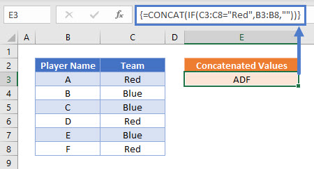
This example will use the CONCAT and IF Functions in an array formula to create a text string of Player Names which relate to a Team value of Red
=CONCAT(IF(C3:C8="Red",B3:B8,""
Users of Excel 2019 will need to enter this formula as an array function by pressing CTRL + SHIFT + ENTER. Users of later versions of Excel do not need to follow this step.
To explain what this formula is doing, lets break it down into steps:
This is our final formula:
=CONCAT(IF(C3:C8="Red",B3:B8,""First, Excel reads the range values into the formula:
=CONCAT(IF({"Red"; "Blue"; "Blue"; "Red"; "Blue"; "Red"}="Red",{"A"; "B"; "C"; "D"; "E"; "F"},""Next the list of Team names is compared to the value Red:
=CONCAT(IF({TRUE; FALSE; FALSE; TRUE; FALSE; TRUE},{"A"; "B"; "C"; "D"; "E"; "F"},""The IF Function replaces TRUE values with the Player Name, and FALSE values with “”
=CONCAT({"A"; ""; ""; "D"; ""; "F"The CONCAT Function then combines all of the array values into one text string:
="ADF"Adding Delimiters or Ignoring Empty Values
If it is required to add delimiting values or text between each value, or for the function to ignore empty cell values, The TEXTJOIN Function can be used instead if you need to add delimiters
Read our TEXTJOIN If article to learn more.
Concatenate If – in pre-Excel 2019
As the CONCAT and TEXTJOIN Functions are not available before the Excel 2019 version, we need to solve this problem in a different way. The CONCATENATE Function is available but does not take ranges of cells as inputs or allow array operations and so we are required to use a helper column with an IF Function instead.
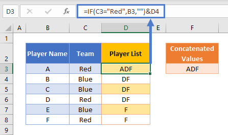
This next example shows how to use a helper column to create a text string of Player Names which relate to a Team value of Red:
=IF(C3="Red",B3,"" &D4
The first step in this example is to use an IF Function to replicate the condition of Team = Red:
=IF(C3="Red",B3,""
Next, we can create a column that builds up a list of these values into one cell by also referencing the cell below it:
=D3&E4
This formula uses the & character to join two values together. Note that the CONCATENATE Function could be used to create exactly the same result, but the & method is often preferred as it is shorter and makes it clearer what action the formula is performing.
These two helper columns can then be combined into one formula:
=IF(C3="Red",B3,""&D4
A summary cell can then reference the first value in the Player List helper column:
=D3Concatenate If in Google Sheets
Google Sheets users should use the TEXTJOIN Function to concatenate values based on a condition.
This example will use the TEXTJOIN and IF Functions to create a text string of Player Names which relate to a Team value of Red
=ARRAYFORMULA(TEXTJOIN("",FALSE,IF(C3:C8="Red",B3:B8,"")))
As this formula requires array inputs for the cell ranges, the ARRAYFORMULA Function should be added to the formula by pressing CTRL + SHIFT + ENTER.
What I am trying to do is concatenate two cells, then check that concatenated value against a column of values, and put an X in a cell if such a value exists. The following equation is what I’m using:
{=IF(CONCATENATE(A2, " ", B2) = 'MasterList'!$C:$C, "x", "")}
Column A is the name of the software and Column B the version number (A="Microsoft .NET Framework 4.5.1", B="4.5.50938", for example). I know that this concatenated value exists on the MasterList worksheet so I don’t understand why I’m not getting the answer I expect.
Gurus, what’s my flaw here?
![]()
0m3r
12.2k15 gold badges33 silver badges70 bronze badges
asked Mar 29, 2017 at 22:24
![]()
The fastest comparison/lookup on the worksheet is a MATCH function. If you have a long column to put this formula into you could try,
=IF(ISNUMBER(MATCH(CONCATENATE(A2, " ", B2), 'MasterList'!$C:$C, 0)), "x", "")
Fill down as necessary.
answered Mar 29, 2017 at 23:04
1
It seams that you select the entire column C on yout MasterListSheet. Don’t you mean just one cell? Like:
=IF(CONCATENATE(A2, " ", B2) = 'MasterList'!$C1, "x", "")
or try to : =IF(CONCATENATE(A2, " ", B2) = MasterList.!$C1, "x", "") (on open Office)
Best thing is instead of you write the Sheet name, let Excel do it for you by editing the formula, remove the sheet name and then with a mouse click navigate to the desired area.
answered Mar 29, 2017 at 22:41
![]()
Alg_DAlg_D
2,2026 gold badges29 silver badges62 bronze badges
I just want to say that before seeing this question, I had no idea what array formulas were.
I have the following working example:
Sheet1:
A1: Microsoft .NET Framework 4.5.1
B1: 4.5.50938

// press control-shift-enter after typing formula
C4: =IF(CONCATENATE(A1," ",B1)=Sheet2!$A:$A,"YAY","NAY")
Sheet2:
A1: Microsoft .NET Framework 4.5.1 4.5.50938
Not sure what the issue is with your spreadsheet. Do the values in MasterList!$C:$C actually correspond to what you expect as the result of the concatenation?
answered Mar 29, 2017 at 22:30
![]()
1
This is not a valid array formula. The LHS is a single cell while the RHS is an array. What it actually does is compare the concatenation to all cells of columns C in MasterList.
You either need to make it a valid array formula or a normal formula. I recommend the second solution.
For the first solution, it should be:
{=IF(CONCATENATE(A:A, " ",B:B ) ='MasterList'!$C:$C, "x", "")}
However, this will be very slow because it will compute and concatenate two full columns, and moreover you will have to select your whole range where you want to calculate it (a full columns) then press Ctrl+Shift+Enter.
You can make it a simple formula in on cell then copy/paste along your column. Formula for C2:
=IF(CONCATENATE(A2, " ", B2) = 'MasterList'!$C2, "x", "")
answered Mar 29, 2017 at 22:39
![]()
A.S.HA.S.H
29k5 gold badges22 silver badges49 bronze badges