
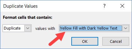
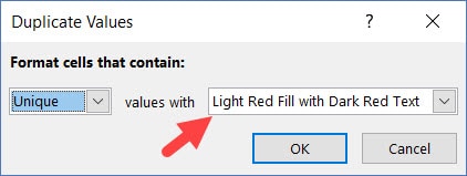
1. Select a data range that you want to compare, and in the Ribbon, go to Home > Conditional Formatting > Highlight Cells Rules > Duplicate Values. 2. In the pop-up window, (1) select Unique and (2) click OK, leaving the default format (Light Red Fill with Dark Red Text).
Contents
- 1 How do I compare two rows in Excel to find differences?
- 2 How do I compare the entire rows in Excel?
- 3 How do I check if two rows match in Excel?
- 4 How do I compare two rows of text in Excel?
- 5 How do you compare rows?
- 6 What is an Xlookup in Excel?
- 7 How do you use the Match function in Excel?
- 8 How do you compare data in two Excel sheets for matches?
- 9 How do I compare cell contents in Excel?
- 10 How do you compare two cells in Excel?
- 11 What is the difference between Xlookup and VLOOKUP?
- 12 Is Xlookup better than VLOOKUP?
- 13 Is Xlookup better than index match?
- 14 How do I see all matches in Excel?
- 15 How do I match properties in Excel?
- 16 What does a Vlookup do?
- 17 Where is spreadsheet compare in Excel?
- 18 How do I compare spreadsheets?
- 19 How do you use Accent 5 cell style in Excel?
- 20 How do you check if a cell contains a specific text in Excel?
How do I compare two rows in Excel to find differences?
To quickly highlight cells with different values in each individual row, you can use Excel’s Go To Special feature.
- Select the range of cells you want to compare.
- On the Home tab, go to Editing group, and click Find & Select > Go To Special… Then select Row differences and click the OK button.
How do I compare the entire rows in Excel?
It is easier to compare just a single cell – so first combine your “whole row” into a single cell. This is easy by concatenating all the cells using the & symbol. Insert a new (hidden) column C on both sheets, that combines the other columns with a formula like: = A1 & B1.
How do I check if two rows match in Excel?
You need an array formula that compares the 2 rows. Instead of pressing Enter after typing the formula, press Ctrl + Shift + Enter , which will tell Excel you want an Array formula. The result will be TRUE if they match and FALSE if they don’t.
How do I compare two rows of text in Excel?
Compare Text
- Use the EXACT function (case-sensitive).
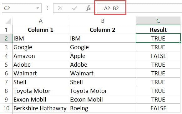
- Use the formula =A1=B1 (case-insensitive).
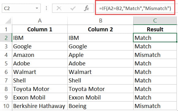
- Add the IF function to replace TRUE and FALSE with a word or message.
- Do you want to compare two or more columns by highlighting the differences in each row?
How do you compare rows?
1. Select a data range that you want to compare, and in the Ribbon, go to Home > Conditional Formatting > Highlight Cells Rules > Duplicate Values. 2. In the pop-up window, (1) select Unique and (2) click OK, leaving the default format (Light Red Fill with Dark Red Text).
What is an Xlookup in Excel?
Use the XLOOKUP function to find things in a table or range by row.With XLOOKUP, you can look in one column for a search term, and return a result from the same row in another column, regardless of which side the return column is on.
How do you use the Match function in Excel?
The MATCH function searches for a specified item in a range of cells, and then returns the relative position of that item in the range. For example, if the range A1:A3 contains the values 5, 25, and 38, then the formula =MATCH(25,A1:A3,0) returns the number 2, because 25 is the second item in the range.
How do you compare data in two Excel sheets for matches?
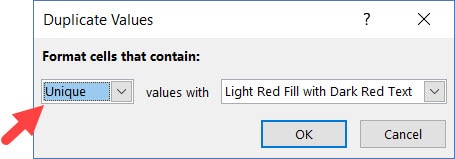
Select both columns of data that you want to compare. On the Home tab, in the Styles grouping, under the Conditional Formatting drop down choose Highlight Cells Rules, then Duplicate Values. On the Duplicate Values dialog box select the colors you want and click OK. Notice Unique is also a choice.
How do I compare cell contents in Excel?
The quickest way to compare two cells is with a formula that uses the equal sign. If the cell contents are the same, the result is TRUE. (Upper and lower case versions of the same letter are treated as equal).
How do you compare two cells in Excel?
Compare Two Columns and Highlight Matches
- Select the entire data set.
- Click the Home tab.
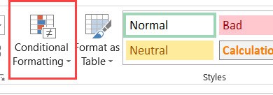
- In the Styles group, click on the ‘Conditional Formatting’ option.
- Hover the cursor on the Highlight Cell Rules option.
- Click on Duplicate Values.
- In the Duplicate Values dialog box, make sure ‘Duplicate’ is selected.
What is the difference between Xlookup and VLOOKUP?
XLOOKUP defaults to an exact match. VLOOKUP defaults to an “approximate” match, requiring that you add the “false” argument at the end of your VLOOKUP to perform an exact match.XLOOKUP can perform horizontal or vertical lookups. The XLOOKUP replaces both the VLOOKUP and HLOOKUP.
Is Xlookup better than VLOOKUP?
The XLOOKUP defaults to an exact match where the VLOOKUP defaults to an approximate match. As the exact match is used most often, this setting would make the XLOOKUP more effective. On top of this, the XLOOKUP offers an additional option of an approximate match returning the next larger value.
Is Xlookup better than index match?
XLOOKUP Vs VLOOKUP Vs INDEX/MATCH
Let’s recap how XLOOKUP outperforms VLOOKUP and INDEX/MATCH: It is the simplest function, with only 3 arguments needed in most cases because the default match_mode is 0 (exact match). It’s a single function, unlike INDEX/MATCH, so it’s faster to type.
How do I see all matches in Excel?
1. Select a blank cell to output the first matched instance, enter the below formula into it, and then press the Ctrl + Shift + Enter keys simultaneously. Note: In the formula, B2:B11 is the range which the matched instances locate in. A2:A11 is the range contains the certain value you will list all instances based on.
How do I match properties in Excel?
Copy cell formatting
- Select the cell with the formatting you want to copy.
- Select Home > Format Painter.
- Drag to select the cell or range you want to apply the formatting to.
- Release the mouse button and the formatting should now be applied.
What does a Vlookup do?
VLOOKUP stands for ‘Vertical Lookup’. It is a function that makes Excel search for a certain value in a column (the so called ‘table array’), in order to return a value from a different column in the same row.
Where is spreadsheet compare in Excel?
Compare two versions of a workbook by using Spreadsheet Compare
- Open Spreadsheet Compare.
- In the lower-left pane, choose the options you want included in the workbook comparison, such as formulas, cell formatting, or macros.
- On the Home tab, choose Compare Files.
How do I compare spreadsheets?
To access the Spreadsheet Compare Add In, click on the Windows icon in the lower left of your task bar, and search for Spreadsheet Compare. You will be taken to a sort of mission control for comparing spreadsheets.
How do you use Accent 5 cell style in Excel?
Apply a cell style
- Select the cells that you want to format. For more information, see Select cells, ranges, rows, or columns on a worksheet.
- On the Home tab, in the Styles group, click Cell Styles.
- Click the cell style that you want to apply.
How do you check if a cell contains a specific text in Excel?
To check if a cell contains specific text, use ISNUMBER and SEARCH in Excel. There’s no CONTAINS function in Excel. 1. To find the position of a substring in a text string, use the SEARCH function.
See all How-To Articles
In this tutorial, you will learn how to compare two rows in Excel and Google Sheets.
Compare Two Rows
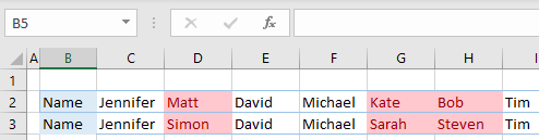
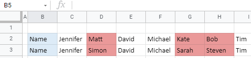
Excel allows you to compare rows and highlight the similarities and differences using conditional formatting. In the following example, there are names in Rows 2 and 3.
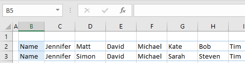
Say you want to compare the two rows above and highlight cells where the rows don’t match (Columns D, G, and H) in red.
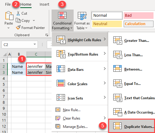
- Select the data range you want to compare, and in the Ribbon, go to Home > Conditional Formatting > Highlight Cells Rules > Duplicate Values.
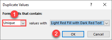
- In the pop-up window, (1) select Unique and (2) click OK, leaving the default format (Light Red Fill with Dark Red Text).
You could also have selected Duplicate and in that case, the same values would be highlighted.
As a result, cells containing different values in Rows 2 and 3 are highlighted in red.
Compare Two Rows in Google Sheets
You can also compare two rows using conditional formatting in Google Sheets.
- Select the data range you want to compare (here, C2:I3), and in the Menu, go to Format > Conditional formatting.
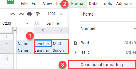
- In the window on the right side, (1) select Custom formula is under Format rules, and (2) enter the formula:
=C$2<>C$3Then (3) click on the fill color icon, (4) choose red, and (5) click Done.
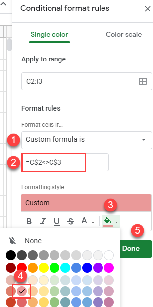
The formula has a dollar sign to fix rows, and only change columns. This means that the formatting rule will go column by column and compare cells in Rows 2 and 3.
As a result, cells with different values have a red fill color.
Содержание
- How to Compare Two Rows in Excel & Google Sheets
- Compare Two Rows
- Compare Two Rows in Google Sheets
- How to compare data in two columns to find duplicates in Excel
- Method 1: Use a worksheet formula
- Method 2: Use a Visual Basic macro
- How to Compare Two Columns in Excel (for matches & differences)
- Compare Two Columns For Exact Row Match
- Example: Compare Cells in the Same Row
- Example: Compare Cells in the Same Row (using IF formula)
- Example: Highlight Rows with Matching Data
- Compare Two Columns and Highlight Matches
- Example: Compare Two Columns and Highlight Matching Data
- Example: Compare Two Columns and Highlight Mismatched Data
- Compare Two Columns and Find Missing Data Points
- Compare Two Columns and Pull the Matching Data
- Example: Pull the Matching Data (Exact)
- Example: Pull the Matching Data (Partial)
How to Compare Two Rows in Excel & Google Sheets
In this tutorial, you will learn how to compare two rows in Excel and Google Sheets.
Compare Two Rows
Excel allows you to compare rows and highlight the similarities and differences using conditional formatting. In the following example, there are names in Rows 2 and 3.
Say you want to compare the two rows above and highlight cells where the rows don’t match (Columns D, G, and H) in red.
- Select the data range you want to compare, and in the Ribbon, go to Home > Conditional Formatting > Highlight Cells Rules > Duplicate Values.
- In the pop-up window, (1) select Unique and (2) click OK, leaving the default format (Light Red Fill with Dark Red Text).
You could also have selected Duplicate and in that case, the same values would be highlighted.
As a result, cells containing different values in Rows 2 and 3 are highlighted in red.
Compare Two Rows in Google Sheets
You can also compare two rows using conditional formatting in Google Sheets.
- Select the data range you want to compare (here, C2:I3), and in the Menu, go to Format > Conditional formatting.
- In the window on the right side, (1) select Custom formula is under Format rules, and (2) enter the formula:
Then (3) click on the fill color icon, (4) choose red, and (5) click Done.
The formula has a dollar sign to fix rows, and only change columns. This means that the formatting rule will go column by column and compare cells in Rows 2 and 3.
As a result, cells with different values have a red fill color.
Источник
How to compare data in two columns to find duplicates in Excel
You can use the following methods to compare data in two Microsoft Excel worksheet columns and find duplicate entries.
Method 1: Use a worksheet formula
In a new worksheet, enter the following data as an example (leave column B empty):
Type the following formula in cell B1:
Select cell B1 to B5.
In Excel 2007 and later versions of Excel, select Fill in the Editing group, and then select Down.
The duplicate numbers are displayed in column B, as in the following example:
Method 2: Use a Visual Basic macro
Warning: Microsoft provides programming examples for illustration only, without warranty either expressed or implied. This includes, but is not limited to, the implied warranties of merchantability or fitness for a particular purpose. This article assumes that you are familiar with the programming language that is being demonstrated and with the tools that are used to create and to debug procedures. Microsoft support engineers can help explain the functionality of a particular procedure. However, they will not modify these examples to provide added functionality or construct procedures to meet your specific requirements.
To use a Visual Basic macro to compare the data in two columns, use the steps in the following example:
Press ALT+F11 to start the Visual Basic editor.
On the Insert menu, select Module.
Enter the following code in a module sheet:
Press ALT+F11 to return to Excel.
Enter the following data as an example (leave column B empty):
Источник
How to Compare Two Columns in Excel (for matches & differences)
Watch Video – Compare two Columns in Excel for matches and differences
The one query that I get a lot is – ‘how to compare two columns in Excel?’.
This can be done in many different ways, and the method to use will depend on the data structure and what the user wants from it.
For example, you may want to compare two columns and find or highlight all the matching data points (that are in both the columns), or only the differences (where a data point is in one column and not in the other), etc.
Since I get asked about this so much, I decided to write this massive tutorial with an intent to cover most (if not all) possible scenarios.
If you find this useful, do pass it on to other Excel users.
This Tutorial Covers:
Note that the techniques to compare columns shown in this tutorial are not the only ones.
Based on your dataset, you may need to change or adjust the method. However, the basic principles would remain the same.
If you think there is something that can be added to this tutorial, let me know in the comments section
Compare Two Columns For Exact Row Match
This one is the simplest form of comparison. In this case, you need to do a row by row comparison and identify which rows have the same data and which ones does not.
Example: Compare Cells in the Same Row
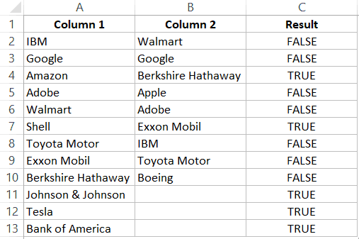
Below is a data set where I need to check whether the name in column A is the same in column B or not.
If there is a match, I need the result as “TRUE”, and if doesn’t match, then I need the result as “FALSE”.
The below formula would do this:
Example: Compare Cells in the Same Row (using IF formula)
If you want to get a more descriptive result, you can use a simple IF formula to return “Match” when the names are the same and “Mismatch” when the names are different.
Note: In case you want to make the comparison case sensitive, use the following IF formula:
With the above formula, ‘IBM’ and ‘ibm’ would be considered two different names and the above formula would return ‘Mismatch’.
Example: Highlight Rows with Matching Data
If you want to highlight the rows that have matching data (instead of getting the result in a separate column), you can do that by using Conditional Formatting.
Here are the steps to do this:
- Select the entire dataset.
- Click the ‘Home’ tab.

- In the Styles group, click on the ‘Conditional Formatting’ option.
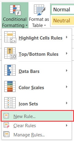
- From the drop-down, click on ‘New Rule’.
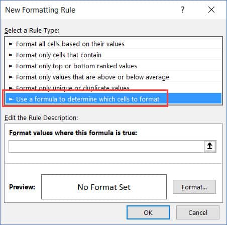
- In the ‘New Formatting Rule’ dialog box, click on the ‘Use a formula to determine which cells to format’.
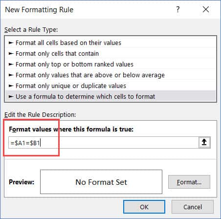
- In the formula field, enter the formula: =$A1=$B1
- Click the Format button and specify the format you want to apply to the matching cells.
- Click OK.
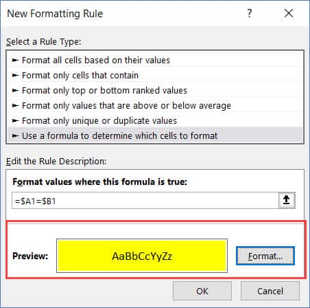
This will highlight all the cells where the names are the same in each row.
Compare Two Columns and Highlight Matches
If you want to compare two columns and highlight matching data, you can use the duplicate functionality in conditional formatting.
Note that this is different than what we have seen when comparing each row. In this case, we will not be doing a row by row comparison.
Example: Compare Two Columns and Highlight Matching Data
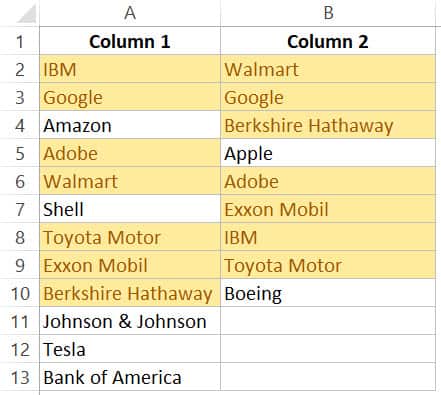
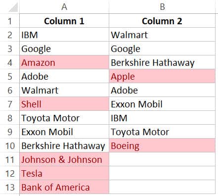
Often, you’ll get datasets where there are matches, but these may not be in the same row.
Something as shown below:
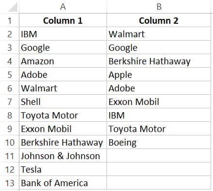
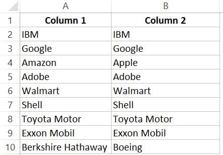
Note that the list in column A is bigger than the one in B. Also some names are there in both the lists, but not in the same row (such as IBM, Adobe, Walmart).
If you want to highlight all the matching company names, you can do that using conditional formatting.
Here are the steps to do this:
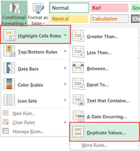
- Select the entire data set.
- Click the Home tab.
- In the Styles group, click on the ‘Conditional Formatting’ option.
- Hover the cursor on the Highlight Cell Rules option.
- Click on Duplicate Values.
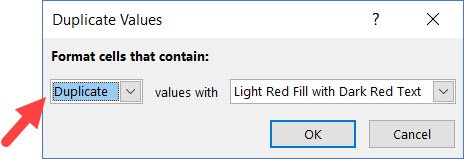
- In the Duplicate Values dialog box, make sure ‘Duplicate’ is selected.
- Specify the formatting.
- Click OK.
The above steps would give you the result as shown below.
Note: Conditional Formatting duplicate rule is not case sensitive. So ‘Apple’ and ‘apple’ are considered the same and would be highlighted as duplicates.
Example: Compare Two Columns and Highlight Mismatched Data
In case you want to highlight the names which are present in one list and not the other, you can use the conditional formatting for this too.
- Select the entire data set.
- Click the Home tab.
- In the Styles group, click on the ‘Conditional Formatting’ option.
- Hover the cursor on the Highlight Cell Rules option.
- Click on Duplicate Values.
- In the Duplicate Values dialog box, make sure ‘Unique’ is selected.
- Specify the formatting.
- Click OK.
This will give you the result as shown below. It highlights all the cells that have a name that is not present on the other list.
Compare Two Columns and Find Missing Data Points
If you want to identify whether a data point from one list is present in the other list, you need to use the lookup formulas.
Suppose you have a dataset as shown below and you want to identify companies that are present in column A but not in Column B,
To do this, I can use the following VLOOKUP formula.
This formula uses the VLOOKUP function to check whether a company name in A is present in column B or not. If it is present, it will return that name from column B, else it will return a #N/A error.
These names which return the #N/A error are the ones that are missing in Column B.
ISERROR function would return TRUE if there is the VLOOKUP result is an error and FALSE if it isn’t an error.
If you want to get a list of all the names where there is no match, you can filter the result column to get all cells with TRUE.
You can also use the MATCH function to do the same;
Note: Personally, I prefer using the Match function (or the combination of INDEX/MATCH) instead of VLOOKUP. I find it more flexible and powerful. You can read the difference between Vlookup and Index/Match here.
Compare Two Columns and Pull the Matching Data
If you have two datasets and you want to compare items in one list to the other and fetch the matching data point, you need to use the lookup formulas.
Example: Pull the Matching Data (Exact)
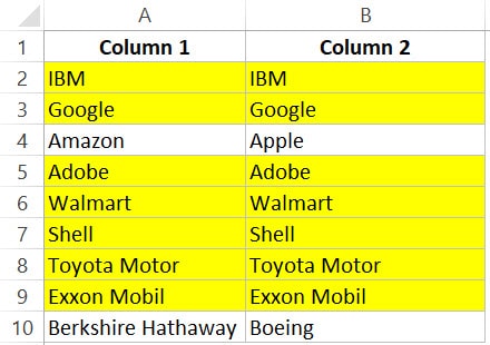
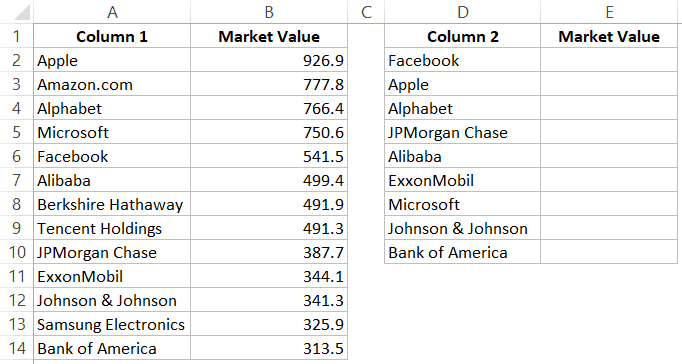
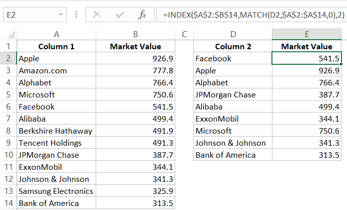
For example, in the below list, I want to fetch the market valuation value for column 2. To do this, I need to look up that value in column 1 and then fetch the corresponding market valuation value.
Below is the formula that will do this:
Example: Pull the Matching Data (Partial)
In case you get a dataset where there is a minor difference in the names in the two columns, using the above-shown lookup formulas is not going to work.
These lookup formulas need an exact match to give the right result. There is an approximate match option in VLOOKUP or MATCH function, but that can’t be used here.
Suppose you have the data set as shown below. Note that there are names that are not complete in Column 2 (such as JPMorgan instead of JPMorgan Chase and Exxon instead of ExxonMobil).
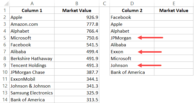
In such a case, you can use a partial lookup by using wildcard characters.
The following formula will give is the right result in this case:
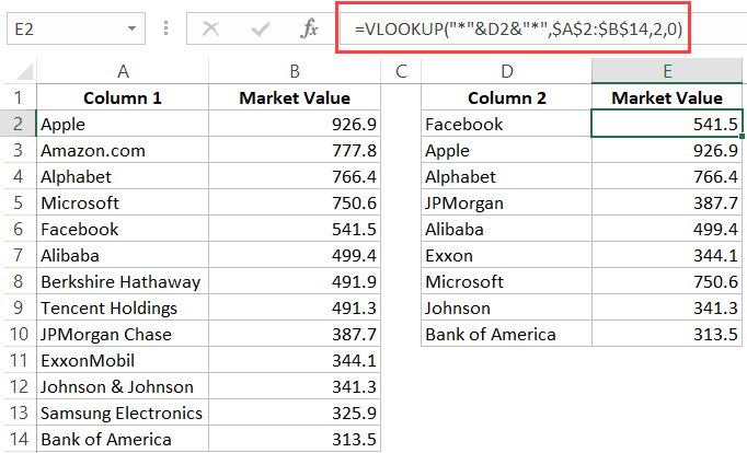
In the above example, the asterisk (*) is a wildcard character that can represent any number of characters. When the lookup value is flanked with it on both sides, any value in Column 1 which contains the lookup value in Column 2 would be considered as a match.
For example, *Exxon* would be a match for ExxonMobil (as * can represent any number of characters).
You May Also Like the Following Excel Tips & Tutorials:
Источник
I’ll put in a sledgehammer-to-crack-a-nut answer here, for completeness, because the question ‘Are these two ranges identical?’ is turning up as an unexamined component of everyone else’s ‘compare my ranges and then do this complicated thing…’ questions.
Your question is a simple question about small ranges. My answer is for large ones; but the question is a good one, and a good place for a more general answer, because it’s simple and clear: and ‘Do these ranges differ?’ and ‘Has someone tampered with my data?’ are relevant to most commercial Excel users.
Most of the answers to the typical ‘compare my rows’ questions are cell-by-cell reads and comparisons in VBA. The simplicity of these answers is commendable, but this approach performs very slowly on a large data sets because:
- Reading a range one cell at a time is very slow;
- Comparing values pair-by-pair is inefficient, especially for strings, when the number of values gets into the tens of thousands,
Point(1) is the important one: it takes the same amount of time for VBA to pick up a single cell using var = Range("A1") as it does to pick up the entire range in one go using var = Range("A1:Z1024")…
…And every interaction with the sheet takes four times as much time as a string comparison in VBA, and twenty times longer than an comparison between floating-point decimals; and that, in turn, is three times longer than an integer comparison.
So your code will probably be four times faster, and possibly a hundred times faster, if you read the entire range in one go, and work on the Range.Value2 array in VBA.
That’s in Office 2010 and 2013 (I tested them); for older version of Excel, you’ll see quoted times between 1/50th and 1/500th of a second, for each VBA interaction with a cell or range of cells. That’ll be way slower because, in both old and new versions of Excel, the VBA actions will still be in single-digit numbers of microseconds: your code will run at least a hundred times faster, and probably thousands of times faster, if you avoid cell-by-cell reads from the sheet in older versions of Excel.
arr1  = Range1.Values
arr2  = Range2.Values

' Consider checking that the two ranges are the same size
' And definitely check that they aren't single-cell ranges,
' which return a scalar variable, not an array, from .Value2

' WARNING: THIS CODE WILL FAIL IF YOUR RANGE CONTAINS AN ERROR VALUE

For i = LBound(arr1, 1) To Ubound(arr1, 2)

    For j = LBound(arr1, 2) To Ubound(arr1, 2)

        If arr1(i, j) <> arr2(i, j) Then
            bMatchFail = True
            Exit For
        End If

    Next j

    If bMatchFail Then Exit For

Next i

Erase arr1
Erase arr2
You’ll notice that this code sample is generic, for two ranges of the same size taken from anywhere — even from separate workbooks. If you’re comparing two adjacent columns, loading a single array of two columns and comparing IF arrX(i, 1) <> arrX(i,2) Then is going to halve the runtime.
Your next challenge is only relevant if you’re picking up tens of thousands of values from large ranges: there’s no performance gain in this extended answer for anything smaller than that.
What we’re doing is:
Using a hash function to compare the values of two large ranges
The idea is very simple, although the underlying mathematics is quite challenging for non-mathematicians: rather than comparing one value at a time, we run a mathematical function that ‘hashes’ the values into a short identifier for easy comparison.
If you’re repeatedly comparing ranges against a ‘reference’ copy, you can store the ‘reference’ hash, and this halves the workload.
There are some fast and reliable hashing functions out there, and they are available in Windows as part of the security and cryptography API. There is a slight problem in that they run on strings, and we have an array to work on; but you can easily find a fast ‘Join2D’ function that gets a string from the 2D arrays returned by a range’s .Value2 property.
So a fast comparison function for two large ranges will look like this:
Public Function RangeCompare(Range1 as Excel.Range, Range2 As Excel.Range) AS Boolean
' Returns TRUE if the ranges are identical.
' This function is case-sensitive.
' For ranges with fewer than ~1000 cells, cell-by-cell comparison is faster

' WARNING: This function will fail if your range contains error values.

RangeCompare = False

If Range1.Cells.Count <> Range2.Cells.Count Then
    RangeCompare = False
ElseIf Range1.Cells.Count = 1 then
    RangeCompare = Range1.Value2 = Range2.Value2
Else
    RangeCompare = MD5(Join2D(Range1.Value2)) = MD5(Join2D(Range2.Value2))
Endif

End Function
I’ve wrapped the Windows System.Security MD5 hash in this VBA function:
Public Function MD5(arrBytes() As Byte) As String
' Return an MD5 hash for any string
' Author: Nigel Heffernan Excellerando.Blogspot.com
' Note the type pun: you can pass in a string, there's no type conversion or cast
' because a string is stored as a Byte array and VBA recognises this.
oMD5 As Object 'Set a reference to mscorlib 4.0 to use early binding
Dim HashBytes() As Byte
Dim i As Integer
Set oMD5 = CreateObject("System.Security.Cryptography.MD5CryptoServiceProvider")
HashBytes = oMD5.ComputeHash_2((arrBytes))
For i = LBound(HashBytes) To UBound(HashBytes)
MD5 = MD5 & Right("00" & Hex(HashBytes(i)), 2)
Next i
Set oMD5 = Nothing ' if you're doing this repeatedly, declare at module level and persist
Erase HashBytes
End Function
There are other VBA implementations out there, but nobody seems to know about the Byte Array / String type pun — they are not equivalent, they are identical — so everyone codes up unnecessary type conversions.
A fast and simple Join2D function was posted by Dick Kusleika on Daily Dose of Excel in 2015:
Public Function Join2D(ByVal vArray As Variant, Optional ByVal sWordDelim As String = " ", Optional ByVal sLineDelim As String = vbNewLine) As String

    Dim i As Long, j As Long
    Dim aReturn() As String
    Dim aLine() As String

    ReDim aReturn(LBound(vArray, 1) To UBound(vArray, 1))
    ReDim aLine(LBound(vArray, 2) To UBound(vArray, 2))

    For i = LBound(vArray, 1) To UBound(vArray, 1)
        For j = LBound(vArray, 2) To UBound(vArray, 2)
            'Put the current line into a 1d array
            aLine(j) = vArray(i, j)
        Next j
        'Join the current line into a 1d array
        aReturn(i) = Join(aLine, sWordDelim)
    Next i

    Join2D = Join(aReturn, sLineDelim)

End Function
If you need to excise blank rows before you make the comparison, you’ll need the Join2D function I posted in StackOverflow back in 2012.
The most common application of this type of hash comparison is for spreadsheet control — change monitoring — and you’ll see Range1.Formula used instead of Range1.Value2: but your question is about comparing values, not formulae.
Footnote: I’ve posted a very similar answer elsewhere. I’d’ve posted it here first if I’d seen this question earlier.
Hay Paula, can you compare lists in Excel?
or
What is the best way to compare two sets of data in Excel?
Very often there is a requirement in Excel to compare two lists, or two data sets to find missing or matching items. As this is Excel, there are always more than one way to do things, including comparing data. From formulas and Conditional Formatting to Power Query. In this article we are going to look at a number ways to compare two lists in Excel and we will also look at comparing entire rows of a data set.
Maybe your preferred way is not included below. If not why don’t you drop a comment below and share with us how you like to compare two lists or datasets in Excel. I look forward to reading your comments.
We wish to compare List 1 with List 2.

Contents
Quick Conditional Formatting to compare two columns of data
Clearing the Conditional Formatting
Match data in Excel using the MATCH function
Compare 2 lists in Excel 365 with MATCH or XMATCH as a Dynamic Array function
MATCH and Dynamic arrays to compare 2 lists
XMATCH Excel 365 to compare two lists
Tables – Comparing lists in Excel where the ranges sizes might change
Highlight differences in Lists using Custom Conditional Formatting
Copy formula to Custom Conditional Formatting
Other Formulas used to compare two lists in Excel
VLOOKUP to compare two lists in Excel
XLOOKUP to compare two lists in Excel
COUNTIF to compare two lists in Excel
How to compare 2 data sets in Excel
Comparing lists or datasets using Power Query

Quick Conditional Formatting to compare two columns of data
Conditional formatting will allow you to highlight a cells or range based on predefined criteria. The quickest and simplest way to visually compare these two columns quickly is to use the predefined highlight duplicate value rule.
Start by selecting the two columns of data.
From the Home tab, select the Conditional Formatting drop down. Then select Highlight Cells Rules. Next select Duplicate values.

A Duplicate Values settings box will open where you can define the formatting and select between Duplicate or Unique values.

By Selecting Duplicate, all reoccurring entries will be set to the selected formatting. Now you can quickly see the items in List 1 that are in List 2 as these are the formatted items. You can also quickly see the items in list 2 that are not in list 1 as these do not have formatting applied.

However, you can also format the Unique items. This can be achieved by selecting Unique from the Duplicate Values setup box.

In this case, we have applied two different conditional formats. The red indicating the duplicates and the green indicating the unique items.
Note, I did not just take the cells with data, I grabbed all of columns A to C. Column B has no data, so it cannot affect the results. However, these cells do contain the conditional formatting applied so it would be better practice to only select the cells you need.
Clearing the Conditional Formatting
To clear all conditional formatting, first select the cell, or range. Then select the conditional formatting drop down on the Home ribbon. Next select Clear Rules. Finally Select Clear Rules from Selected Cells.

If you have more than one conditional formatting applied at once and you only want to remove one of these, select Manage Rules from the conditional formatting drop down. Select the rule you want to delete and then select Delete Rule.

By pressing OK, the rule will removed from the Rules Manager and the cells will no longer contain the formatting.

So that is the most basic way you can compare two lists in Excel. Its quick, its simple and it is effective. You can also apply conditional formatting based on formulas, which we will look at later in this article.
Match data in Excel using the MATCH function
There are many lookup formulas that you can use to compare two ranges or lists in Excel. The first we will look at is the MATCH function.
The MATCH function returns the relative position in a list. A number based on its position, if found, in the lookup array.
The syntax for MATCH is
=MATCH (lookup value, Lookup array, Match type)
Where lookup value is the value you want to find a match for. Lookup array is the list in which you are looking for a match. And Match type allows you to select between an exact or approximate match.
We want to write a match formula to see if the items in List 2 are in List 1.
In cell E3 we can enter the formula
=MATCH(C2, $A$2:$A$21,0)

By filling this formula down, for the values where Excel finds a match, the position of that match will be returned. Where there is no match the return value will be an #N/A.

Very often, the relative position or the #N/A is of no value to us and we need to convert these values into true or false. To do this we can easily expand on our Match formula using a logical function. As Match returns a number, we can use the ISNUMBER function
=ISNUMBER(MATCH(C2, $A$2:$A$21,0))

Compare 2 lists in Excel 365 with MATCH or XMATCH as a Dynamic Array function
If you are using Excel 365 you have further alternatives when using MATCH to compare lists or data. As Excel 365 thinks in arrays, we can now pass an array as the lookup value of MATCH and our results will spill for us. This removes the need to copy the formula down and with only 1 formula, your spreadsheet will be less prone to errors and more compact.
MATCH and Dynamic arrays to compare 2 lists
If you are not yet familiar with Dynamic Arrays, I would suggest you have a read of this article: Excel Dynamic Arrays – A new way to model your Excel Spreadsheets: to get a better understand on how they work and spill ranges.
The only change to the match formula is instead of selecting cell C2 as our lookup value we will select the range C2:12
=ISNUMBER(MATCH (C2:C12,$A$2:$A$21,0))

As you can see, the one formula spills the results down column E.
XMATCH Excel 365 to compare two lists
Excel 365 also introduces the new function XMATCH. Just like the MATCH function XMATCH returns a relative position in a list. Now you are familiar XLOOKUP, which replaces the old VLOOKUP function, you know XLOOKUP comes with additional power. This come in the form of new conditions in the formula syntax such as search mode and match types. Well, XMATCH also as this extra power over its predecessor MATCH.
The syntax for XMATCH is
XMATCH (Lookup Value, Lookup Array, [Match Mode],[Search Mode])
Where
Lookup Value is the value you are looking to find the relative position
Lookup Array is the row or column that contains the Lookup Value
Match mode is optional. Unlike the old MATCH function, the default is an exact match. You can also select between
- Exact match or next smallest
- Exact match or next largest
- Wildcard match
Search mode is also optional. The default (and only option in the old MATCH function) is to look from the top down. You can also select last to first and binary searches. If you are working with binary searches. The wildcard match option does not work.
With XMATCH we can use either Dynamic arrays or cell references to create the formula, just like we have looked at with MATCH. For this example, we will use Dynamic Arrays. The formula is very similar to what we used with MATCH; except we do not have to select 0 for an exact match as in XMATCH this is the default setting. Let us mix things up a little this time a look at finding items in list 2 not in list one.
In this case we can use the formula
=NOT(ISNUMBER(XMATCH(C2:C12,A2:A21)))
Where not will turn trues into false and false into trues.

Tables – Comparing lists in Excel where the ranges sizes might change
In each of the formulas we have looked at so far, we have selected a range of cells in our Match functions that is not dynamic. That means if we add new data to one of the lists, we have a manual step to update our formula to include the new data.
To convert the lists to tables, select one of the lists and press CTRL. This is the keyboard shortcut to convert to a table. If you selected the header in the range of cells, ensure you tick the box to confirm your table has headers.

Tables by their nature use structured naming. Therefore, when you are writing a formula and you select a column from a table, it will not show cell references, but the column name.
Looking at our previous formula using XMATCH to find items in list 2 not in list 1, we can re-write this function now using our table references
=NOT (ISNUMBER(XMATCH(list2[List 2],list1[List 1])))

Now, as we have used tables, if we add a new row to either of the tables, our spill range will also increase to include the new data.

Highlight differences in Lists using Custom Conditional Formatting
Earlier in this article we looked at a very quick way of comparing these two lists using a predefined rule for duplicates. We can however also use Custom Conditional Formatting. If you are not familiar with Custom Conditional Formatting, I would suggest you check out this article: Excel Dynamic Conditional Formatting Tricks:
We need to look at two different approaches here to highlighting differences. When we are not using tables and we have created a true/false formula to identify the differences, we can take a copy of the formula and add this to our Custom formatting. However, with Tables we need to force the use of cell references.
Copy formula to Custom Conditional Formatting
Start by taking a copy of the formula. As we have tested the formula in the spreadsheet, we can see that it works before we use it in conditional formatting. This is best practice as very often with relative and absolute cell references it can be difficult to get the formula correct.

Select the cells that you want to apply the custom formatting to. Then from the Home ribbon select the conditional formatting drop down and select New Rule

The New Formatting Rule set up box will open and select Use Formula to determine which cells to format. Then paste in the formula and set the formatting type

This will result in all cells that are in both lists being formatted to your chosen format.

Keep in mind that we selected a range of cells to apply this conditional formatting and it is not dynamic. Should we use tables, this would update without the need to change anything!
Other Formulas used to compare two lists in Excel
There are many formulas you can use to compare two lists in Excel. We have already looked at MATCH and XMATCH, but now we are going to look at a few more. Any of the lookup functions will really work along with some others!
VLOOKUP to compare two lists in Excel
If you are not familiar with VLOOKUP, you can read about it here. Simply put VLOOKUP will return a corresponding value from a cell, if there is no corresponding value an #N/A error will be returned. In our example we are working with text. So, we can carry out a VLOOKUP and test to see if it returns text. If we were using numbers then we could replace ISTEXT with ISNUMBER.
We could use the function =ISTEXT(VLOOKUP(C2, $A$2:$A$21,1,FALSE))

Or if we were using Dynamic arrays in Excel 365, we could use the function
=ISTEXT(VLOOKUP (C2:C12,$A$2:$A$21,1,FALSE))

XLOOKUP to compare two lists in Excel
XLOOKUP was introduced in Excel 365 and you can find out more about it here. Very much like VLOOKUP, XLOOKUP will return a corresponding value from a cell, and you can define a result if the value is not found. Using Dynamic arrays, the function would be
=ISTEXT(XLOOKUP (C2:C12,A2:A21,A2:A21))

COUNTIF to compare two lists in Excel
The COUNTIF function will count the number of times a value, or text is contained within a range. If the value is not found, 0 is returned. We can combine this with an IF statement to return our true and false values.
=IF(COUNTIF (A2:A21,C2:C12)<>0,”True”, “False”)

How to compare 2 data sets in Excel
Comparing two lists is easy enough and we have looked now at several ways to do this. But comparing two data sets can be a little more difficult.
Let us look at an example. We have two tables of data, each containing the same column headers. Looking at the image, we can see matching these two tables would require looking at more than one column.

When you need to look at more than one column, the solution would be to create a composite column combining the data into one column. This will create a unique column for each row which we can then use as the matching column
In this example we could combine the Name and DoB to give each table a unique identifier
There are many ways to join contents of a cell, in this case we will do a simple concatenate. As we are using tables, the formula will shoe the table naming format.
=[@Name] &”-“&[@DoB]

Repeat the steps on the second table.
Now we can use any of the examples above to match these two new columns of data. Where they match, we know they match the entire row.

Comparing lists or datasets using Power Query
You can also compare lists and datasets using Excels Power Query. By connecting to the tables and then merging the tables, using different join types we can compare both lists.
In this video you will learn how to compare or reconcile two different data sets using Excels Power query
There is a data set to go along with this video and practice along which you can grab from this article.
However very often you will have datasets where there is no matching column and we need to create a column to carry out a reconciliation between two different lists or two different data sources. In this video you will learn how to create a matching column using power query so you can then compare the data.