Excel compare sheet to sheet

Compare two or more worksheets at the same time

Excel for Microsoft 365 Excel for the web Excel 2021 Excel 2019 Excel 2016 Excel 2013 Excel 2010 Excel 2007 More…Less

You can quickly compare two worksheets in the same workbook or in different workbooks by viewing them side by side. You can also arrange multiple worksheets to view them all at the same time.

On the View tab, in the Window group, click New Window.
On the View tab, in the Window group, click View Side by Side .
In each workbook window, click the sheet that you want to compare.
To scroll both worksheets at the same time, click Synchronous Scrolling in the Window group on the View tab.

Note: This option is available only when View Side by Side is turned on.

Tips:

If you resize the workbook windows for optimal viewing, you can click Reset Window Position to return to the original settings.
To restore a workbook window to full size, click Maximize at the upper-right corner of the workbook window.

Open both of the workbooks that contain the worksheets that you want to compare.
On the View tab, in the Window group, click View Side by Side .

If you have more than two workbooks open, Excel displays the Compare Side by Side dialog box. In this dialog box, under Compare Side by Side with, click the workbook that contains the worksheet that you want to compare with your active worksheet, and then click OK.
In each workbook window, click the sheet that you want to compare.
To scroll both worksheets at the same time, click Synchronous Scrolling in the Window group on the View tab.

Note: This option is available only when View Side by Side is turned on.

Tips:

Beginning with Excel 2013, workbooks that you open in Excel are no longer displayed as multiple workbook windows inside a single Excel window. Instead, they are shown as separate Excel windows. Because workbooks don’t share the same Excel window, they are displayed with their own ribbon, and you can view the open workbooks on different monitors.
If you resize the workbook windows for optimal viewing, you can click Reset Window Position to return to the original settings.
To restore a workbook window to full size, click Maximize at the upper-right corner of the workbook window.

Open one or more workbooks that contain the worksheets that you want to view at the same time.
Do one of the following:
- If the worksheets that you want to view are in the same workbook, do the following:
  1. Click a worksheet that you want to view.
  2. On the View tab, in the Window group, click New Window.
  3. Repeat steps 1 and 2 for each sheet that you want to view.
- If the worksheets that you want to view are in different workbooks, continue with step 3.
On the View tab, in the Window group, click Arrange All.
Under Arrange, click the option that you want.
If the sheets that you want to view are all located in the active workbook, select the Windows of active workbook check box.

Tip: To restore a workbook window to full size, click Maximize at the upper-right corner of the workbook window.

On the View tab, in the Window group, click New Window.
In each workbook window, click the sheet that you want to compare.

Need more help?

You can always ask an expert in the Excel Tech Community or get support in the Answers community.

Просмотр рядом, чтобы сравнить таблицы.

Если у вас относительно небольшие файлы и вы внимательны к деталям, этот быстрый и простой способ сравнения может вам подойти. Я говорю о режиме «Просмотр рядом», который позволяет расположить два окна Excel рядом. Вы можете использовать этот метод для визуального сравнения двух таблиц или двух листов из одной книги.

Сравните 2 книги.

Предположим, у вас есть отчеты о продажах за два месяца, и вы хотите просмотреть их оба одновременно, чтобы понять, какие товары показали лучшие результаты в этом месяце, а какие — в прошлом.

Чтобы просмотреть два файла Эксель рядом, сделайте следующее:

Откройте оба файла.
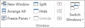
Перейдите на вкладку «Вид» и нажмите кнопку «Рядом». (1) Это оно!

По умолчанию два отдельных окна Excel отображаются горизонтально.

Чтобы разделить окна по вертикали, нажмите кнопку «Упорядочить все» (3) и выберите «Рядом» (4):

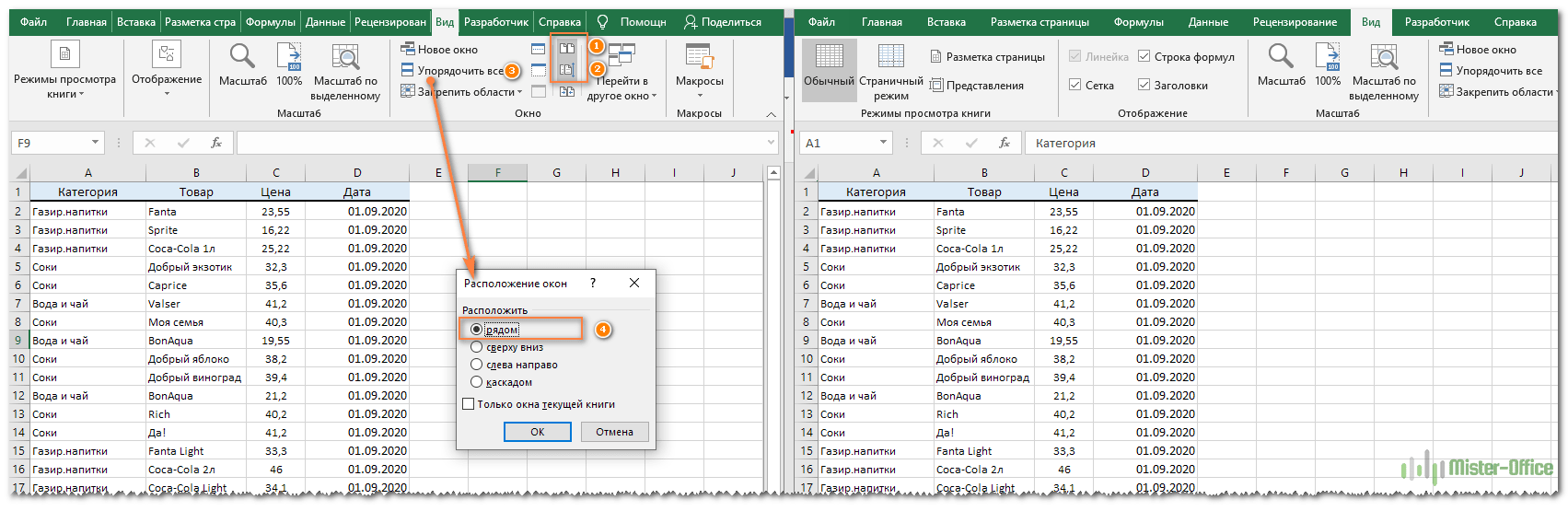
В результате два отдельных окна будут расположены, как на скриншоте.

Если вы хотите прокручивать оба листа одновременно, чтобы сравнивать данные строка за строкой, убедитесь, что параметр синхронной прокрутки (2) включен. Он обычно включается автоматически, как только вы активируете режим одновременного просмотра двух книг.

Расположите рядом несколько таблиц Excel.

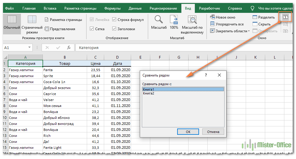
Чтобы просматривать более двух файлов одновременно, откройте все книги, которые вы хотите сравнить, и нажмите кнопку «Рядом».

Появится диалоговое окно «Сравнить рядом», в котором вы выберете файлы, которые будут отображаться вместе с активной книгой.

Чтобы просмотреть все открытые файлы одновременно, нажмите кнопку «Упорядочить все» и выберите предпочтительное расположение: мозаичное, горизонтальное, вертикальное или каскадное.

Для небольших таблиц вы легко сможете визуально сравнить их данные. Хотя, конечно, риск ошибки из-за человеческого фактора здесь присутствует.

Сравните два листа в одной книге.

Иногда 2 листа, которые вы хотите сравнить, находятся в одной книге. Чтобы просмотреть их рядом, выполните следующие действия.

Откройте файл, перейдите на вкладку «Вид» и нажмите кнопку «Новое окно».

Это действие откроет тот же файл в дополнительном окне.
Включите режим просмотра «Рядом», нажав соответствующую кнопку на ленте.
Выберите лист 1 в первом окне и лист 2 во втором окне.

Быстрое выделение значений, которые различаются.

Это также не очень обременительный способ. Если вам просто нужно найти и удостовериться в наличии или же отсутствии отличий между записями, вам нужно на вкладке «Главная», выбрать кнопку «Найти и выделить», предварительно выделив диапазон, где надо сравнить данные в Эксель.

В открывшемся меню выберите пункт «Выделить группу ячеек…» и в появившемся диалоговом окне выберите «отличия по строкам».

К сожалению, это нормально работает только для сравнения 2 столбцов (или строк), а не всей таблицы целиком. Кроме того, строки должны быть одинаковым образом отсортированы, поскольку ячейки сравниваются построчно. Если у вас товары отсортированы по-разному, либо вообще различный ассортимент, то никакой пользы от этого метода не будет.

Формула сравнения.

Это самый простой способ соотнесения таблиц в Excel, который позволяет идентифицировать в них ячейки с разными значениями.

Простейший вариант – сопоставление двух таблиц, находящихся на одном листе. Можно соотносить как числовые, так и текстовые значения, всего-навсего прописав в одной из соседних ячеек формулу их равенства. В результате при тождестве ячеек мы получим сообщение ИСТИНА, в противном случае — ЛОЖЬ.

Предположим, у нас имеется два прайс-листа (старый и новый), в которых на некоторые товары различаются цены. При этом порядок следования товаров одинаков. Поэтому мы можем при помощи простейшей формулы прямо на этом же листе сравнить идентичные ячейки с данными.

=G3=C3

Результатом будет являться либо ИСТИНА (в случае совпадения), либо ЛОЖЬ (при отрицательном результате).

Таким же образом можно производить сравнение данных в таблицах, которые расположены на разных листах. Процедура сравнения практически точно такая, как была описана выше, кроме того факта, что при создании формулы придется переключаться между листами. В нашем случае выражение будет иметь следующий вид:

=G3=Лист2!C3

Если ваши таблицы достаточно велики, то довольно утомительно будет просматривать колонку I на предмет поиска слова ЛОЖЬ. Поэтому может быть полезным сразу определить — а есть ли вообще несовпадения?

Можно подсчитать общее количество расхождений и сразу вывести это число где-нибудь отдельно.

=СУММПРОИЗВ(—(C3:C25<>G3:G25))

или можно сделать это формулой массива

{=СУММ(—(C3:C25<>G3:G25))}

Если формула возвращает ноль, значит, данные полностью совпадают. Ну а ежели результат положительный, то нужны более детальные исследования. О них мы и поговорим далее.

Как произвести сравнение на отдельном листе.

Чтобы сравнить два листа Эксель на предмет различий, просто откройте новый пустой лист, введите следующую формулу в ячейку A1, а затем скопируйте ее вниз и вправо, перетащив маркер заполнения:

=ЕСЛИ(Лист1!A1 <> Лист2!A1; «Лист1:»&Лист1!A1&» — Лист2:»&Лист2!A1; «»)

Поскольку мы используем относительные ссылки на ячейки, формула будет меняться в зависимости от расположения столбца и строки. В результате формула в A1 будет сравнивать ячейки A1 в Лист1 и Лист2, формула в B1 будет сравнивать ячейку B1 на обоих листах и так далее. Результат будет выглядеть примерно так:

В результате вы получите отчет о различиях на новом листе. Думаю, это достаточно информативно.

Как вы можете видеть на приведенном выше рисунке, формула сравнивает 2 листа, находит ячейки с разными значениями и отображает различия в соответствующих местах.

Обратите внимание, что в отчете о различиях (ячейка D4) даты представлены числами, поскольку в таком виде они хранятся во внутренней системе Excel, что не очень удобно для анализа различий между ними.

Как сравнить две таблицы при помощи формулы ВПР.

Предположим, у нас снова 2 прайс-листа. Однако, в отличие от предыдущего примера, они содержат разное количество товаров, да и сами товары расположены в произвольном порядке. Поэтому описанный выше способ, когда мы построчно сравнивали две таблицы, здесь не сработает.

Нам необходимо последовательно взять каждый товар из одной таблицы, найти его во второй, извлечь оттуда его цену и сравнить с первоначальной ценой. Здесь нам не обойтись без формул поиска. Поможет нам функция ВПР.

Для наглядности расположим обе таблицы на одном листе.

Формула

=ЕСЛИОШИБКА(ВПР(F3;$B$3:$C$18;2;0);0)

берёт наименование товара из второго прайса, ищет его в первом, и в случае удачи извлекает соответствующую цену из первой таблицы. Она будет записана рядом с новой ценой в столбце H. Если поиск завершился неудачей, то есть такого товара ранее не было, то ставим 0. Таким образом, старая и новая цена оказываются рядом, и их легко сравнить простейшей операцией вычитания. Что и сделано в столбце I.

Аналогично можно сопоставлять и данные на разных листах. Просто нужно соответствующим образом изменить ссылки в формуле, указав в них имя листа.

Вот еще один пример. Возьмём за основу более новую информацию, то есть второй прайс. Выведем только сведения о том, какие цены и на какие товары изменились. А то, что не изменилось, выводить в итоговом отчёте не будем.

Разберём действия пошагово. Формула в ячейке J3 ищет наименование товара из первой позиции второй таблицы внутри первой. Если таковое найдено, извлекается соответствующая этому товару старая цена и сразу же сравнивается с новой. Если они одинаковы, то в ячейку записывается пустота «».

=ЕСЛИ(ЕСЛИОШИБКА(ВПР(F3;$B$3:$C$18;2;0);0)=G3;»»;ЕСЛИОШИБКА(ВПР(F3;$B$3:$C$18;2;0);0))

Таким образом, в ячейке J3 будет указана старая цена, если ее удастся найти, а также если она не равна новой.

Далее если ячейка J3 не пустая, то в I3 будет указано наименование товара —

=ЕСЛИ(J3<>»»;F3;»»)

а в K3 – его новая цена:

=ЕСЛИ(J3<>»»;G3;»»)

Ну а далее в L3 просто найдем разность K3-J3.

Таким образом, в отчёте сравнения мы видим только несовпадения значений второй таблицы по сравнению с первой.

И еще один пример, который может быть полезен. Попытаемся сравнить в итоговой таблице оба прайс-листа с эталонным общим списком товаров.

В ячейке B2 запишем формулу

=ЕСЛИ(ЕНД(ВПР(A2;Прайс1!$B$3:$B$19;1;0));»Нет»;ВПР(A2;Прайс1!$B$3:$C$19;2;0))

Так мы выясним, какие цены из второй таблицы встречаются в первой.

Для каждой цены из первого прайса проверяем, совпадает ли она с новыми данными —

=ЕСЛИ(ЕНД(ВПР(A2;Прайс2!$B$3:$B$22;1;0));»Нет»;ВПР(A2;Прайс2!$B$3:$C$22;2;0))

Эталонный список находится у нас в столбце A. В результате мы получили своего рода сводную таблицу цен – старых и новых.

Еще несколько примеров использования функции ВПР для сравнения таблиц вы можете найти в этой статье.

Выделение различий между таблицами цветом.

Чтобы закрасить ячейки с разными значениями на двух листах выбранным вами цветом, используйте функцию условного форматирования Excel:

На листе, где вы хотите выделить различия, выберите все используемые ячейки. Для этого щелкните верхнюю левую ячейку используемого диапазона, обычно A1, и нажмите Ctrl + Shift + End, чтобы расширить выделение до последней использованной ячейки.
На вкладке Главная кликните Условное форматирование > Новое правило и создайте его со следующей формулой:

=A1<>Лист2!A1

Где Лист2 — это имя другого листа, который вы сравниваете с текущим.

В результате ячейки с разными значениями будут выделены выбранным вами цветом:

Если вы не очень хорошо знакомы с условным форматированием, вы можете найти подробные инструкции по созданию правила в следующем руководстве: Условное форматирование Excel в зависимости от значения ячейки.

Сравнение при помощи сводной таблицы.

Хороший вариант сравнения — объединить таблицы в единую сводную, и там уже сопоставлять данные между собой.

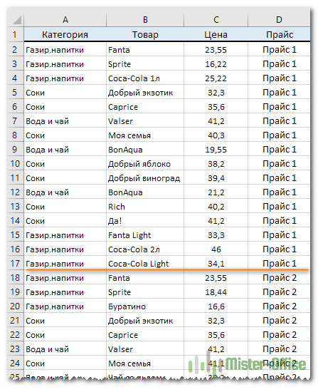
Вернемся к нашему примеру с двумя прайс-листами. Объединим наши данные на одном листе. Чтобы отличить данные одной таблицы от другой, добавим вспомогательный столбец D и укажем в нем, откуда именно взяты данные:

А теперь приступим к созданию сводной таблицы. Я не буду подробно останавливаться на том, как мы это будем делать. Все шаги подробно описаны в статье Как сделать сводную таблицу в Excel.

Поместим поле Товар в область строк, поле Прайс в область столбцов и поле Цена в область значений.

Как видно на скриншоте ниже, для каждого товара, встречающегося хотя бы в одном из прайсов, указана цена.

Сводная таблица автоматически сформирует общий список всех товаров из старого и нового прайсов и сортирует их по алфавиту. Причём, без повторов. У новых товаров нет старой цены, у удаленных товаров — новой цены. Легко увидеть изменения цен, если таковые были.

Общие итоги здесь смысла не имеют, и их можно отключить на вкладке Конструктор — Общие итоги — Отключить для строк и столбцов.

Если изменятся цены, то достаточно просто обновить созданную сводную, щелкнув по ней правой кнопкой мыши — Обновить. А вот если изменится список товаров или добавится новый файл для сравнения, то придется заново формировать исходный массив или же добавлять в него новые данные.

Плюсы: такой подход на порядок быстрее работает с большими объемами данных, чем ВПР. Можно сравнить данные нескольких таблиц.

Минусы: надо вручную копировать данные в одну большую таблицу и добавлять столбец с названием исходного файла.

Сравнение таблиц с помощью Power Query

Power Query — это бесплатная надстройка для Microsoft Excel, позволяющая загружать в него данные практически из любых источников и преобразовывать потом их желаемым образом. В Excel 2016 эта надстройка уже встроена по умолчанию на вкладке Данные, а для более ранних версий ее нужно отдельно скачать с сайта Microsoft и установить.

Перед загрузкой наших прайс-листов в Power Query их необходимо преобразовать сначала в умные таблицы. Для этого выделим диапазон с данными и нажмем на клавиатуре сочетание Ctrl+T или выберем на ленте вкладку Главная — Форматировать как таблицу. Имена созданных таблиц можно изменить на вкладке Конструктор (я оставлю стандартные Таблица1 и Таблица2, которые генерируются по умолчанию).

Загрузите первый прайс в Power Query с помощью кнопки Из таблицы/диапазона на вкладке Данные.

После загрузки вернемся обратно в Excel из Power Query командой Закрыть и загрузить — Закрыть и загрузить в…

В появившемся затем окне выбираем «Только создать подключение».

Повторите те же действия с новым прайс-листом.

Теперь создадим третий запрос, который будет объединять и сравнивать данных из предыдущих двух. Для этого выберем на вкладке Данные — Получить данные — Объединить запросы — Объединить. Все шаги вы видите на скриншоте ниже.

В окне объединения выберем в выпадающих списках наши таблицы, выделим в них столбцы с названиями товаров и в нижней части определим способ объединения — Полное внешнее.

После нажатия на ОК должна появиться таблица из четырёх столбцов, где в четвертой колонке нужно развернуть вложенное содержимое с помощью двойной стрелки в шапке.

После нажатия вы увидите список столбцов из второго прайса. Выбираем Товар и Цена. Получаем следующую картину:

А теперь сравним цены. Идем на вкладку Добавление столбца и жмем на кнопку Условный столбец. А затем в открывшемся окне вводим несколько условий проверки с соответствующими им значениями, которые нужно отобразить:

Теперь осталось вернуться на вкладку Главная и нажать Закрыть и загрузить.

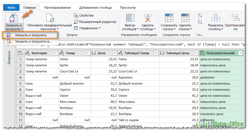
Получаем новый лист в нашей рабочей книге:

Примечание. Если в будущем в наших прайс-листах произойдут любые изменения (добавятся или удалятся строки, изменятся цены и т.д.), то достаточно будет лишь обновить наши запросы сочетанием клавиш Ctrl+Alt+F5 или кнопкой Обновить все на вкладке Данные.

Ведь все данные извлекаются из «умных» таблиц Excel, которые автоматически меняют свой размер при добавлении либо удалении из них какой-либо информации. Однако, помните, что имена столбцов в исходных таблицах не должны меняться, иначе получим ошибку «Столбец такой-то не найден!» при попытке обновить запрос.

Это, пожалуй, самый красивый и удобный способ из всех стандартных. Шустро работает с большими таблицами. Не требует ручных правок при изменении размеров.

Как видите, есть несколько способов сравнить две таблицы Excel, используя формулы или условное форматирование. Однако эти методы не подходят для комплексного сравнения из-за следующих ограничений:

Они находят различия только в значениях, но не могут сравнивать формулы или форматирование ячеек.
Многие из них не могут идентифицировать добавленные или удаленные строки и столбцы. Как только вы добавите или удалите строку / столбец на одном листе, все последующие строки / столбцы будут отмечены как отличия.
Они хорошо работают на уровне листа, но не могут обнаруживать структурные различия на уровне книги Excel, к примеру добавление и удаление листов.

Эти проблемы решаются путем использования дополнений к Excel, о чем мы поговорим далее.

Как сравнить таблицы при помощи Ultimat Suite для Excel

Последняя версия Ultimate Suite включает более 60 новых функций и улучшений, самым интересным из которых является «Сравнение таблиц» — инструмент для сравнения листов или диапазонов данных в Excel.

Чтобы сделать сравнение более интуитивным и удобным, надстройка разработана следующим образом:

Мастер шаг за шагом проведет вас через процесс и помогает настраивать различные параметры.
Вы можете выбрать алгоритм сравнения, наиболее подходящий для ваших наборов данных.
Вместо отчета о различиях сравниваемые листы отображаются в режиме просмотра различий, чтобы вы могли сразу просмотреть все различия и управлять ими по очереди.

Теперь давайте попробуем использовать этот инструмент на наших примерах электронных таблиц из предыдущего примера и посмотрим, отличаются ли результаты.

Нажмите кнопку «Сравнить листы (Compare Two Sheets)» на вкладке «Данные Ablebits » в группе « Объединить »:

Появится окно мастера с предложением выбрать два листа, которые вы хотите сравнить на предмет различий.

По умолчанию выбираются все листы, но вы также можете выбрать текущую таблицу или определенный диапазон , нажав соответствующую кнопку:

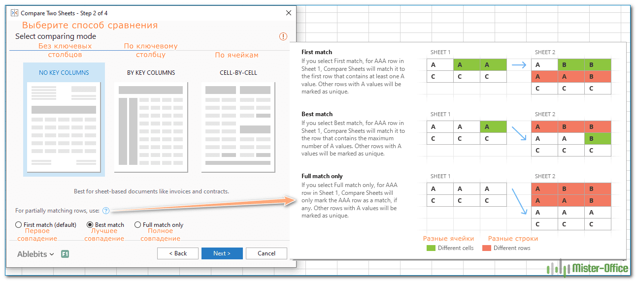
На следующем шаге вы выбираете алгоритм сравнения:
- Без ключевых столбцов (по умолчанию) — лучше всего подходит для сложных документов, таких как счета-фактуры или контракты.
- По ключевым столбцам — подходит для таблиц, организованных по столбцам, которые имеют один или несколько уникальных идентификаторов, таких как номера заказов или артикулы товаров.
- По ячейке — лучше всего использовать для сравнения таблиц с одинаковым макетом и размером, таких как балансы или статистические отчеты.

Совет. Если вы не уверены, какой алгоритм подходит вам, выберите вариант по умолчанию (без ключевых столбцов). Какой бы алгоритм вы ни выбрали, надстройка найдет все различия, только выделит их по-разному (целые строки или отдельные ячейки).

На этом же шаге вы можете выбрать предпочтительный тип соответствия:

Первое совпадение (по умолчанию) — сравнивает строку на листе 1 с первой найденной строкой на листе 2, которая имеет хотя бы одну совпадающую ячейку.
Наилучшее совпадение — сравнивает строку на листе 1 со строкой на листе 2, которая имеет максимальное количество совпадающих ячеек.
Полное совпадение — находит на обоих листах строки, которые имеют одинаковые значения во всех ячейках, и отмечает все остальные строки как уникальные.

В этом примере мы сначала будем искать наилучшее совпадение, используя режим сравнения без ключевых столбцов, который установлен по умолчанию.

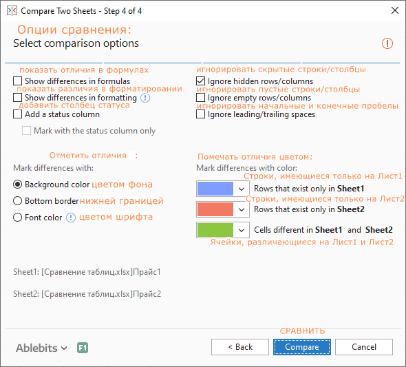
На следующем шаге укажите, какие различия следует выделить, а какие игнорировать, и как помечать различия.

Скрытые строки и столбцы не имеют значения, и мы говорим надстройке игнорировать их:

Нажмите кнопку «Сравнить (Compare)» и подождите немного, пока программа обработает ваши данные и создаст их резервные копии. Резервные копии всегда создаются автоматически, поэтому вы можете не беспокоиться о сохранности своих данных.

После обработки листы открываются друг рядом с другом в специальном режиме просмотра различий с выбранным способом выделения отличий:

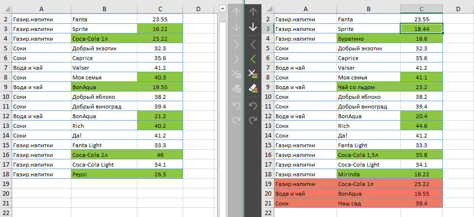
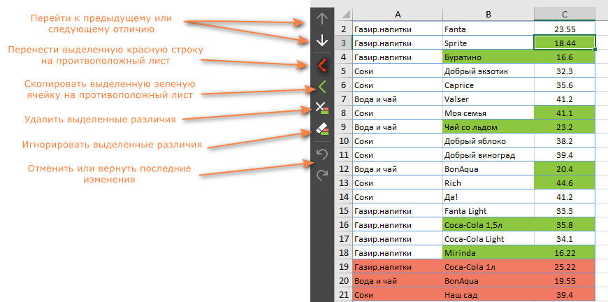
На скриншоте выше различия выделены цветами по умолчанию:

Красные строки — строки, существующие только на Листе 2 (справа).
Зеленые ячейки — различные ячейки в частично совпадающих строках.

А вот если мы выберем второй алгоритм сравнения — по ключевому столбцу, то нам будет предложено указать его. В нашем случае вполне можно ключевым столбцом обозначить «Товар».

После этого мы видим немного другой результат сравнения:

Как видите, основным здесь действительно является факт совпадения значений в столбцах B. Строки, в которых нет такого совпадения, сразу выделяются красным или фиолетовым. А вот если совпадение есть, тогда идем в столбец С и сравниваем записанную там цену. Зелёные ячейки как раз и показывают нам товары, которые имеются в обоих прайс-листах, но цена на них изменилась.

Не знаю как вам, но мне второй вариант представляется более информативным.

А что же дальше делать с этим сравнением?

Чтобы помочь вам просматривать различия и управлять ими, на каждом листе есть собственная вертикальная панель инструментов. Для неактивного рабочего листа (справа на нашем скриншоте) эта панель отключена. Чтобы активировать панель инструментов, просто выберите любую ячейку на соответствующем листе.

Используя её, вы последовательно просматриваете найденные различия и решаете, объединить их или игнорировать:

Как только последнее различие будет устранено, вам будет предложено сохранить книги и выйти из режима просмотра различий.

Если вы еще не закончили обработку различий, но хотели бы сделать перерыв, нажмите кнопку «Выйти из просмотра различий» в нижней части панели инструментов и выберите один из следующих вариантов:

Сохраните внесенные вами изменения и сохраните оставшиеся различия (Save workbooks and keep difference marks),
Сохраните внесенные вами изменения и удалите оставшиеся различия (Save workbooks and remove difference marks),
Восстановите исходные книги из резервных копий (Restore workbooks from backup copies).

Вот как вы можете сравнить два листа в Excel при помощи инструмента сравнения Compare Two Sheets (надеюсь, он вам понравился

Если вам интересно попробовать, полнофункциональная ознакомительная версия доступна для загрузки здесь .

Источник

17 авг. 2022 г.
читать 2 мин

Иногда вам может понадобиться сравнить два разных листа Excel, чтобы определить различия между ними.

К счастью, это довольно легко сделать, и этот урок объясняет, как это сделать.

Как определить различия между двумя листами Excel

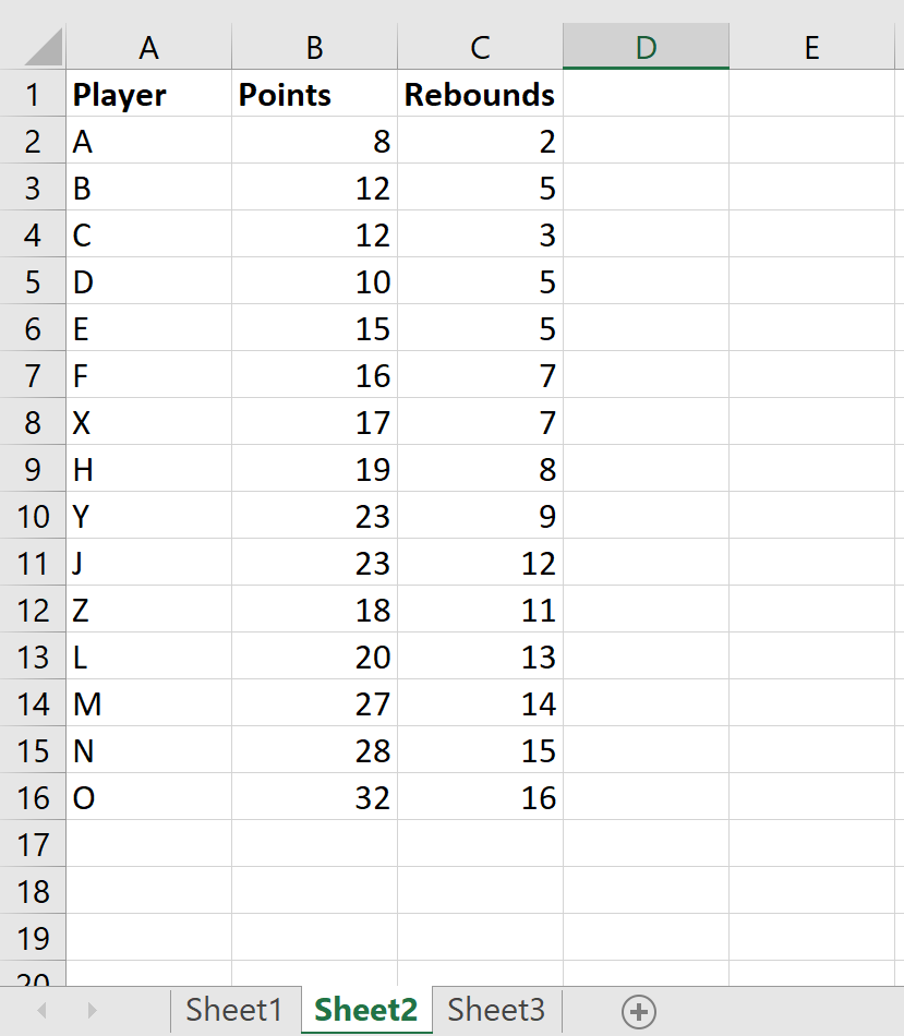
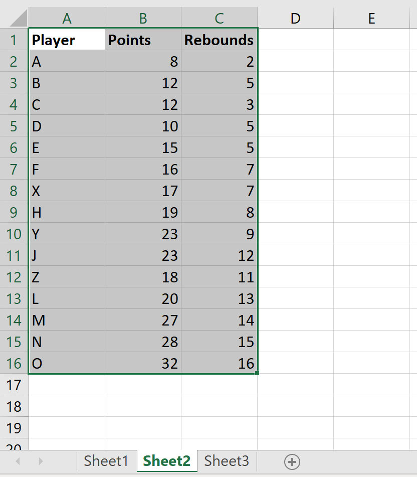
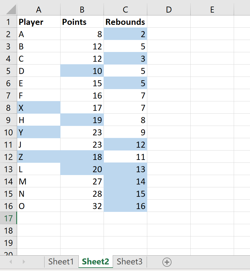
Предположим, у нас есть следующие два листа в Excel с некоторой информацией о баскетболистах:

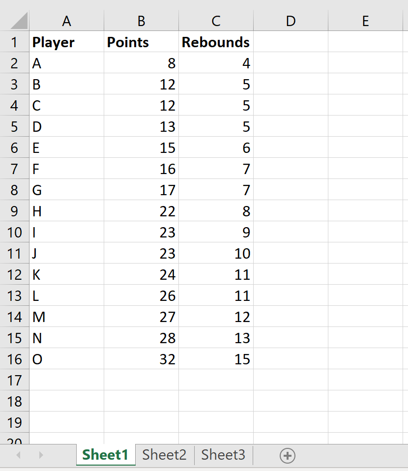
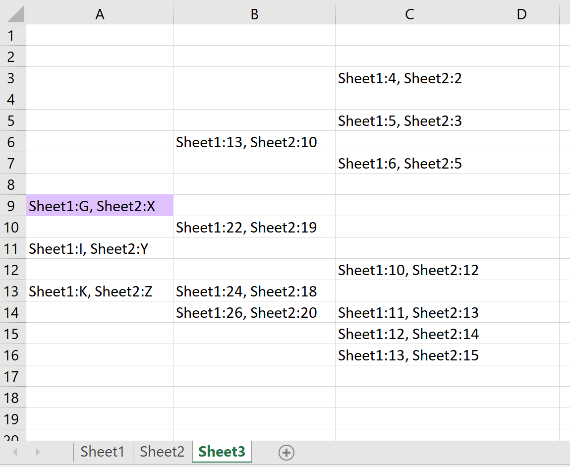
Чтобы сравнить различия между двумя листами, мы можем создать третий лист и использовать следующую формулу в ячейке A2:

=IF(Sheet1!A1 <> Sheet2!A1, "Sheet1:"&Sheet1!A1&", Sheet2:"&Sheet2!A1, "")

Затем мы можем скопировать эту формулу в каждую ячейку, что приведет к следующему:

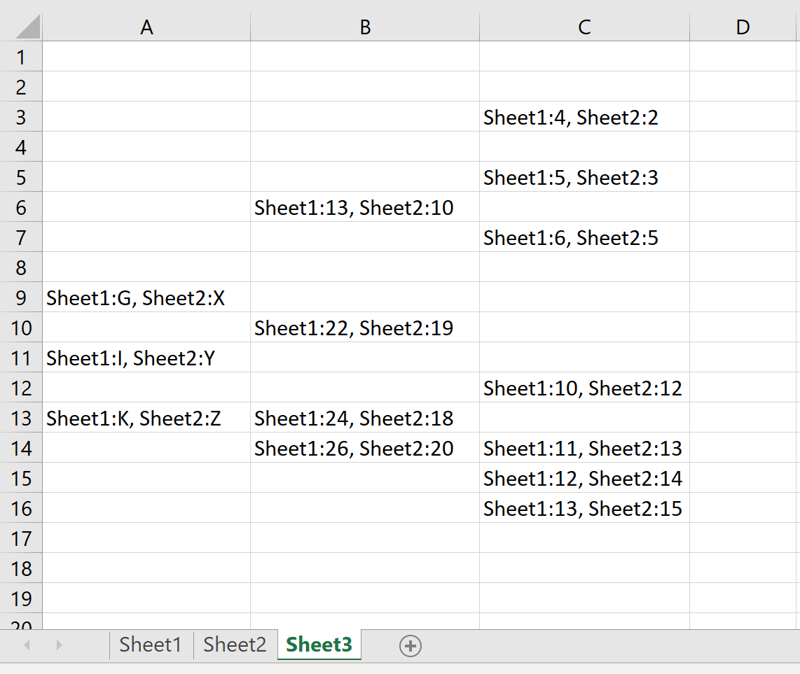
Если соответствующие ячейки на Листе1 и Листе2 идентичны, ячейка на Листе3 будет пустой. Однако, если ячейки на двух листах различаются, различия будут показаны на Листе3.

Например, ячейка A9 на первом листе имеет значение G , а ячейка A9 на втором листе имеет значение X :

Как выделить различия между двумя листами Excel

Помимо определения различий между двумя листами, вы также можете выделить различия с помощью условного форматирования.

Например, предположим, что мы хотим выделить каждую ячейку на Листе2, которая имеет значение, отличное от соответствующей ячейки на Листе1. Для этого мы можем использовать следующие шаги:

Шаг 1: Выберите диапазон ячеек.

Сначала выделите весь диапазон ячеек, к которым мы хотим применить условное форматирование:

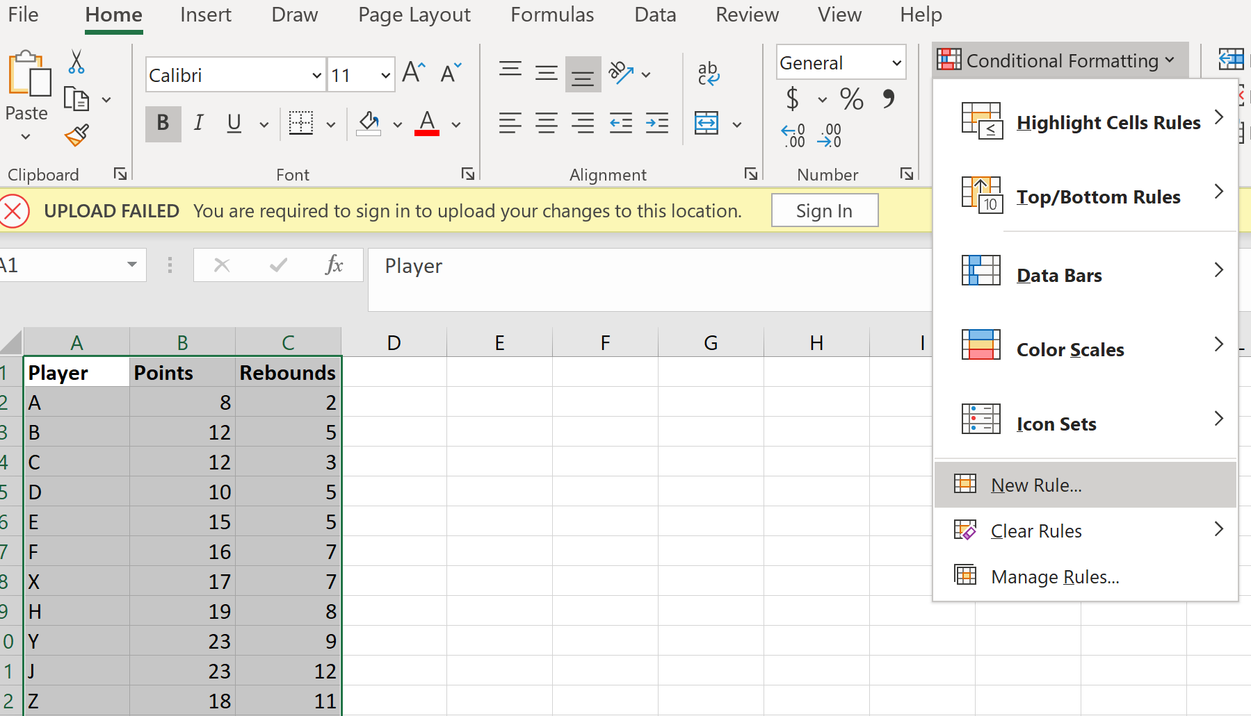
Шаг 2: Выберите условное форматирование.

Затем на вкладке « Главная » в группе « Стили » нажмите « Условное форматирование », а затем нажмите « Новое правило» .

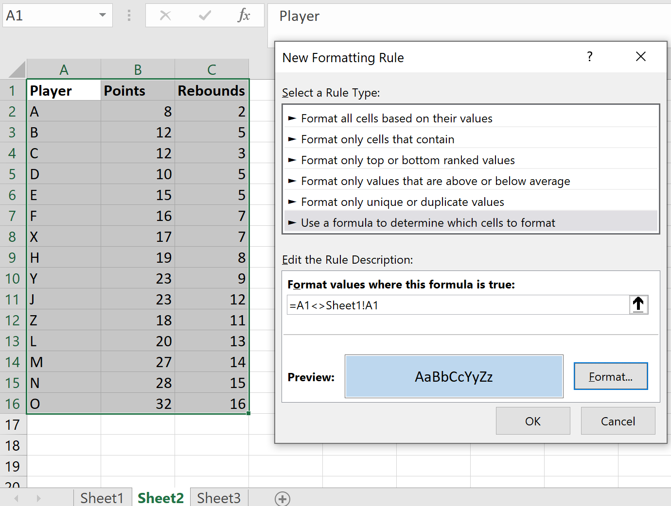
Шаг 3: Выберите условное форматирование.

Выберите параметр « Использовать формулу для определения форматируемых ячеек».Затем введите следующую формулу:

=A1<>Sheet1!A1

Затем нажмите « Формат» и выберите цвет, который вы хотите использовать, чтобы выделить разные ячейки. Затем нажмите ОК .

После того, как вы нажмете OK , будут выделены ячейки на Листе2, значения которых отличаются от соответствующих ячеек на Листе1:

Вы можете найти больше учебников по Excel здесь .

Источник

Watch Video – How to Compare Two Excel Sheets for Differences

Comparing two Excel files (or comparing two sheets in the same file) can be tricky as an Excel workbook only shows one sheet at a time.

This becomes more difficult and error-prone when you have a lot of data that needs to be compared.

Thankfully, there are some cool features in Excel that allow you to open and easily compare two Excel files.

In this Excel tutorial, I will show you multiple ways to compare two different Excel files (or sheets) and check for differences. The method you choose will depend on how your data is structured and what kind of comparison you’re looking for.

Let’s get started!

Compare Two Excel Sheets in Separate Excel Files (Side-by-Side)

If you want to compare two separate Excel files side by side (or two sheets in the same workbook), there is an in-built feature in Excel to do this.

It’s the View Side by Side option.

This is recommended only when you have a small dataset and manually comparing these files is likely to be less time-consuming and error-prone. If you have a large dataset, I recommend using the conditional method or the formula method covered later in this tutorial.

Let’s see how to use this when you have to compare two separate files or two sheets in the same file.

Suppose you have two files for two different months and you want to check what values are different in these two files.

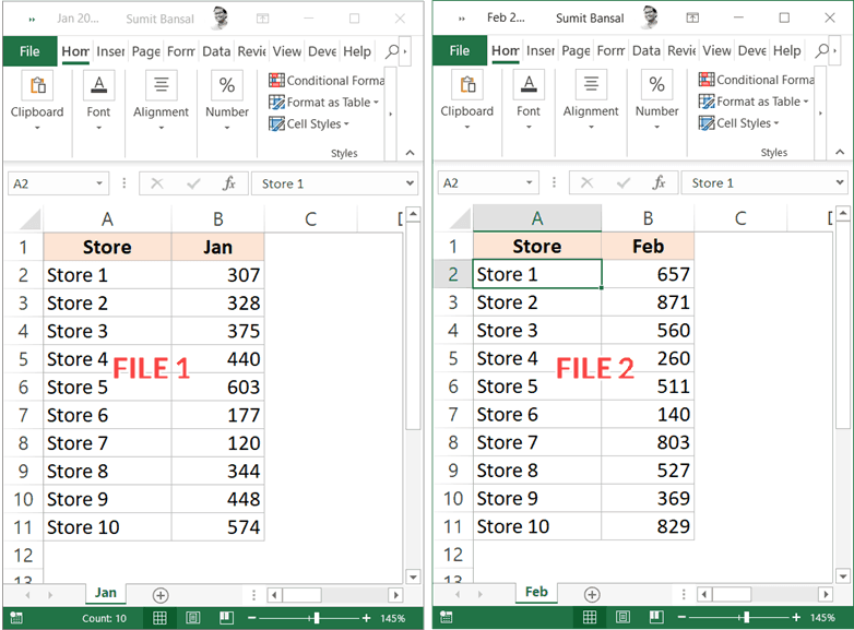
By default, when you open a file, it’s likely to take up your entire screen. Even if you reduce the size, you always see one Excel file at the top.

With the view side-by-side option, you can open two files and then arrange these horizontally or vertically. This allows you to easily compare the values without switching back and forth.

Below are the steps to align two files side by side and compare them:

Open the files that you want to compare.
In each file, select the sheet that you want to compare.
Click the View tab
In the Windows group, click on the ‘View Side by Side’ option. This becomes available only when you have two or more Excel files open.

As soon as you click on the View side by side option, Excel will arrange the workbook horizontally. Both of the files will be visible, and you’re free to edit/compare these files while they are arranged side by side.

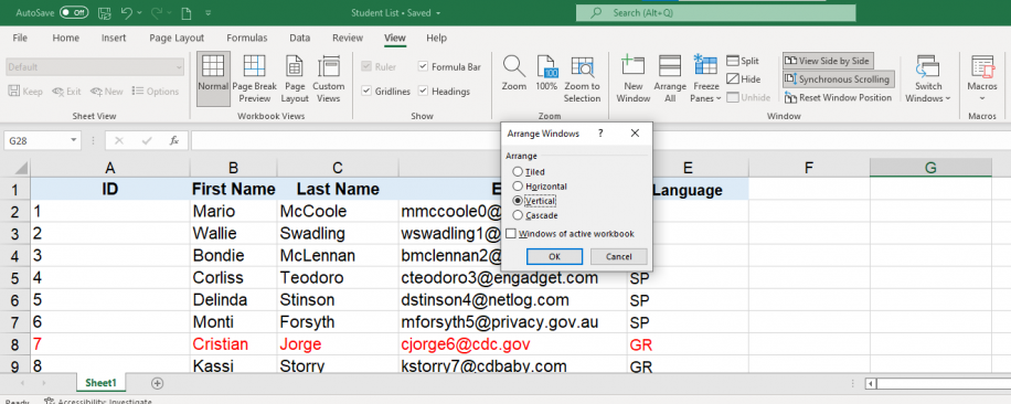
In case you want to arrange the files vertically, click on the Arrange All option (in the View tab).

This will open the ‘Arrange Windows’ dialog box where you can select ‘Vertical’.

At this point, if you scroll down in one of the worksheets, the other one would remain as is. You can change this so that when you scroll in one sheet, the other also scrolls at the same time. This makes it easier to do a line by line comparison and spot any differences.

But to do this, you need to enable Synchronous Scrolling.

To enable Synchronous Scrolling, click on the View tab (in any of the workbooks) and then click on the Synchronous Scrolling option. This is a toggle button (so if you want to turn it off, simply click on it again).

Comparing Multiple Sheets in Separate Excel Files (Side-by-Side)

With the ‘View Side by Side’ option, you can only compare two Excel file at one go.

In case you have multiple Excel files open, when you click on the View Side by Side option, it will show you a ‘Compare Side by Side’ dialog box, where you can choose which file you want to compare with the active workbook.

In case you want to compare more than two files at one go, open all these files and then click on the Arrange All option (it’s in the View tab).

In the Arrange Windows dialog box, select Vertical/Horizontal and then click OK.

This will arrange all the open Excel files in the selected order (vertical or horizontal).

Compare Two Sheets (Side-by-Side) in the Same Excel Workbook

In case you want to compare two separate sheets in the same workbook, you can’t use the View side by side feature (as it works for separate Excel files only).

But you can still do the same side-by-side comparison.

This is made possible by the ‘New Windows’ feature in Excel, that allows you to open two instances on the same workbook. Once you have two instances open, you can arrange these side by side and then compare these.

Suppose you have an Excel workbook that has two sheets for two different months (Jan and Feb) and you want to compare these side by side to see how the sales per store have changed:

Below are the steps to compare two sheets in Excel:

Open the workbook that has the sheets that you want to compare.
Click the View tab
In the Window group, click on the ‘New Window’ option. This opens the second instance of the same workbook.
In the ‘View’ tab, click on ‘Arrange All’. This will open the Arrange Windows dialog box
Select ‘Vertical’ to compare data in columns (or select Horizontal if you want to compare data in rows).
Click OK.

The above steps would arrange both the instances of the workbook vertically.

At this point in time, both the workbooks would have the same worksheet selected. In one of the workbooks, select the other sheet that you want to compare with the active sheet.

How does this work?

When you click on New Window, it opens the same workbook again with a slightly different name. For example, if your workbook name is ‘Test’ and you click on New Window, it will name the already open workbook ‘Test – 1’ and the second instance as ‘Test – 2’.

Note that these are still the same workbook. If you make any changes in any of these workbooks, it would be reflected in both.

And when you close any one instance of the open file, the name would revert back to the original.

You can also enable synchronous scrolling if you want (by clicking on the ‘Synchronous Scrolling’ option in the ‘View’ tab)

Compare Two Sheets and Highlight Differences (Using Conditional Formatting)

While you can use the above method to align the workbooks together and manually go through the data line by line, it’s not a good way in case you have a lot of data.

Also, doing this level of comparison manually can lead to a lot of errors.

So instead of doing this manually, you can use the power of Conditional Formatting to quickly highlight any differences in the two Excel sheets.

This method is really useful if you have two versions in two different sheets and you want to quickly check what has changed.

Note that you CAN NOT compare two sheets in different workbooks.

Since Conditional Formatting can not refer to an external Excel file, the sheets you need to compare needs to be in the same Excel workbook. In case these aren’t, you can copy a sheet from the other file to the active workbook and then make this comparison.

For this example, suppose you have a dataset as shown below for two months (Jan and Feb) in two different sheets and you want to quickly compare the data in these two sheets and check if the prices of these items have changed or not.

Below are the steps to do this:

Select the data in the sheet where you want to highlight the changes. Since I want to check how prices have changed from Jan to Feb, I have selected the data in the Feb sheet.
Click the Home tab
In the Styles group, click on ‘Conditional Formatting’
In the options that show up, click on ‘New Rule’
In the ‘New Formatting Rule’ dialog box, click on ‘Use a formula to determine which cells to format’
In the formula field, enter the following formula: =B2<>Jan!B2
Click the Format button
In the Format Cells dialog box that shows up, click on the ‘Fill tab’ and select the color in which you want to highlight the mismatched data.
Click OK
Click OK

The above steps would instantly highlight any changes in the dataset in both the sheets.

How does this work?

Conditional formatting highlights a cell when the given formula for that cell returns a TRUE. In this example, we are comparing each cell in one sheet with the corresponding cell in the other sheet (done using the not equal to operator <> in the formula).

When conditional formatting finds any difference in the data, it highlights that in the Jan sheet (the one in which we have applied the conditional formatting.

Note that I have used relative reference in this example (A1 and not $A$1 or $A1 or A$1).

When using this method to compare two sheets in Excel, remember the following;

This method is good to quickly identify differences, but you can’t use it on an on-going basis. For example, if I enter a new row in any of the datasets (or delete a row), it would give me incorrect results. As soon as I insert/delete the row, all subsequent rows are considered as different and highlighted accordingly.
You can only compare two sheets in the same Excel file
You can only compare the value (not the difference in formula or formatting).

Compare Two Excel Files/Sheets And Get The Differences Using Formula

If you’re only interested in quickly comparing and identifying the differences between two sheets, you can use a formula to fetch only those values that are different.

For this method, you will need to have a separate worksheet where you can fetch the differences.

This method would work if want to compare two separate Excel workbook or worksheets in the same workbook.

Let me show you an example where I am comparing two datasets in two sheets (in the same workbook).

Suppose you have the dataset as shown below in a sheet called Jan (and similar data in a sheet called Feb), and you want to know what values are different.

To compare the two sheets, first, insert a new worksheet (let’s call this sheet ‘Difference’).

In cell A1, enter the following formula:

=IF(Jan!A1<>Feb!A1,"Jan Value:"&Jan!A1&CHAR(10)&"Feb Value:"&Feb!A1,"")

Copy and paste this formula for a range so that it covers the entire dataset in both the sheets. Since I have a small dataset, I will only copy and paste this formula in A1:B10 range.

The above formula uses an IF condition to check for differences. In case there is no difference in the values, it will return blank, and in case there is a difference, it will return the values from both the sheets in separate lines in the same cell.

The good thing with this method is that it only gives you the differences and show you exactly what the difference is. In this example, I can easily see that the price in cell B4 and B8 are different (as well as the exact values in these cells).

Compare Two Excel Files/Sheets And Get The Differences Using VBA

If you need to compare Excel files or sheets quite often, it’s a good idea to have a ready Excel macro VBA code and use it whenever you need to make the comparison.

You can also add the macro to the Quick Access Toolbar so that you can access with a single button and instantly know what cells are different in different files/sheets.

Suppose you have two sheets Jan and Feb and you want to compare and highlight differences in the Jan sheet, you can use the below VBA code:

Sub CompareSheets()
Dim rngCell As Range
 
For Each rngCell In Worksheets("Jan").UsedRange

    If Not rngCell = Worksheets("Feb").Cells(rngCell.Row, rngCell.Column) Then
        rngCell.Interior.Color = vbYellow
    End If

Next rngCell

End Sub

The above code uses the For Next loop to go through each cell in the Jan sheet (the entire used range) and compares it with the corresponding cell in the Feb sheet. In case it finds a difference (which is checked using the If-Then statement), it highlights those cells in yellow.

You can use this code in a regular module in the VB Editor.

And if you need to do this often, it’s better to save this code in the Personal Macro workbook and then add it to the Quick Access toolbar. In those ways, you will be able to do this comparison with a click of a button.

Here are the steps to get the Personal Macro Workbook in Excel (it’s not available by default so you need to enable it).

Here are the steps to save this code in the Personal Macro Workbook.

And here you will find the steps to add this macro code to the QAT.

Using a Third-Party Tool – XL Comparator

Another quick way to compare two Excel files and check for matches and differences is by using a free third-party tool such as XL Comparator.

This is a web-based tool where you can upload two Excel files and it will create a comparison file that will have the data that is common (or different data based on what option you selected.

Suppose you have two files that have customer datasets (such as name and email address), and you want to quickly check what customers are there is file 1 and not in file 2.

Below is how you compare two Excel files and create a comparison report:

Open https://www.xlcomparator.net/
Use the Choose file option to upload two files (maximum size of each file can be 5MB)
Click on the Next button.
Select the common column in both these files. The tool will use this common column to look for matches and differences
Select one of the four options, whether you want to get matching data or different data (based on File 1 or File 2)
Click on Next
Download the comparison file which will have the data (based on what option you selected in step 5)

Below is a video that shows how XL Comparator tool works.

One concern you may have when using a third-party tool to compare Excel files is about privacy.

If you have confidential data and privacy is really important for it, it’s better to use other methods shown above.

Note that the XL Comparator website mentions that they delete all the files after 1 hour of doing the comparison.

These are some of the methods you can use to compare two different Excel files (or worksheets in the same Excel file). Hope you found this Excel tutorial useful.

You may also like the following Excel tutorials:

How to Compare Two Columns in Excel (for matches & differences)
How to Remove Duplicates in Excel
How to Compare Text in Excel (Easy Formulas)
Split Each Excel Sheet Into Separate Files (Step-by-Step)
Combine Data from Multiple Workbooks in Excel
Combine Data From Multiple Worksheets into a Single Worksheet in Excel
How to Compare Dates in Excel (Greater/Less Than, Mismatches)

Источник

One of the most common scenarios when working with Excel spreadsheets is having files with similar or duplicate data. The reasons for this could be many, but it usually involves spending a considerable amount of time checking complete files or separate worksheets manually.

This article will explain how to compare two or multiple Excel files, as well as two Excel sheets, for differences. To achieve this, we will describe how to use three useful methods to spot differences in a quick and easy way; these include side-by-side viewing, conditional formatting rules, and the =IF formula.

How to compare two Excel files using side-by-side view?

We will start by illustrating how to compare two Excel workbooks using the side-by-side view. However, we recommend using this method in case your dataset is not too large; if not, we recommend using one of the two methods outlined further on in this article. This is how you can compare two Excel files using the side-by-side viewing feature.

1. Open the two Excel workbooks you would like to compare and go to View > View Side by Side on any of the opened files.

How to compare two Excel files — View side by side

2. By default, Excel will place both files horizontally, as shown below.

How to compare two Excel files — Horizontal view

3. To arrange them vertically, click “Arrange All”, and then select “Vertical”.

How to compare two Excel files — Arrange vertically

4. The two Excel files will now be arranged vertically, as shown below.

How to compare two Excel files — Vertical view

5. Make sure that the “Synchronous Scrolling” option is activated since this will allow you to scroll through the data on both files simultaneously and allow you to compare more easily. Although it activates automatically as soon as you enable the side-by-side view, you can also check that it’s activated in your toolbar within the “Window” group.

How to compare two Excel files — Synchronous Scrolling

Now that we know how easy it is to compare two Excel files, let’s see how we can apply this viewing method to Excel sheets.

How to Combine Multiple Excel Files Into One

Discover the most popular methods used to manually or automatically combine multiple Excel spreadsheets and data inputs into one master file

How to compare two Excel sheets using side-by-side view?

Sometimes, similar or duplicate data may appear within the same spreadsheet. IF you want to avoid having to switch from one sheet to another to compare the data, this is how you can quickly compare two Excel sheets side by side.

1. Open the Excel file where you would like to compare sheets. Then, go to View > New Window.

How to compare two Excel files — View New Window

2. You will now have the same Excel file open up in a different window, as shown below.

How to compare two Excel files — Same file in New Window

3. Select “View Side by Side” and make sure to select a different sheet on each file. As before, you can select vertical or horizontal viewing according to your preference.

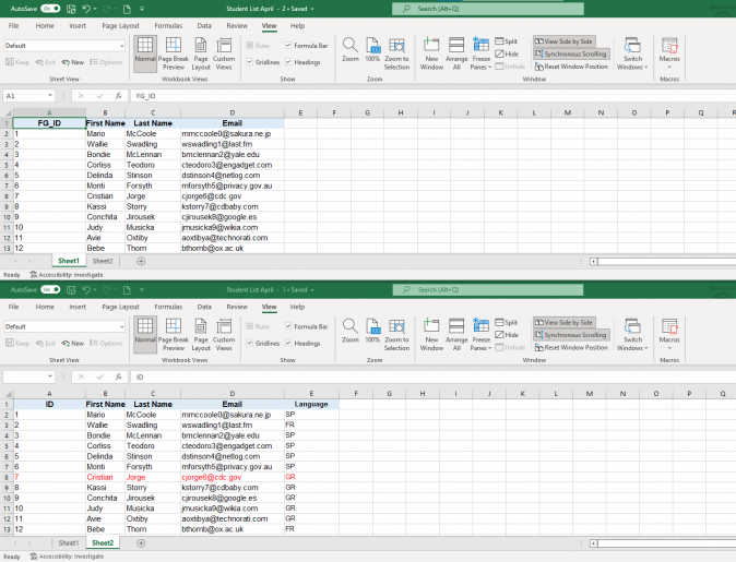
How to compare two Excel files — Sheet 1 and 2

So far, you have seen how easy it is to compare two files and sheets on Excel. However, what if you would like to compare more than two files at the same time? This is how you can compare multiple Excel files using the side-by-side view.

How to compare multiple Excel files using side-by-side view?

Comparing multiple files for differences follows a similar process and will only take you a few simple steps.

1. Open all the Excel workbooks you would like to compare and go to View > View Side by Side. Select the file you want to start comparing with in the “Compare Side by Side” dialog box.

How to compare two Excel files — Compare side by side

2. Click “Arrange All” to view all the opened files at the same time.

How to compare two Excel files — Arrange All

3. Then, select the type of arrangement according to your preference. Here, I have chosen the “Tiled” arrangement.

How to compare two Excel files — Tiled arrangement

So far, these methods are useful in case your datasets are not too large and easily manageable. If you want to compare larger datasets for differences in values, the best way is to use the =IF formula or a conditional formatting rule. Let’s explore the =IF formula first.

How to compare two Excel sheets using a formula?

This is the most straightforward way to compare data between two Excel sheets. This formula will allow you to identify cells containing different values, and a comparative report will be generated in a new worksheet.

1. Open a new empty sheet in your Excel workbook and enter the following formula in cell A1: =IF(Sheet1!A1 <> Sheet2!A1, «Sheet1:»&Sheet1!A1&» vs Sheet2:»&Sheet2!A1, «»)

How to compare two Excel files — Enter IF formula

2. Grab the bottom-right corner of the formula cell, and drag down.

How to compare two Excel files — A1 cell comparison in Sheets

The formula will adapt to the column and row position it fills. This way, the formula in cell A1 compares to cell A1 in “Sheet1” and “Sheet2”; the formula in cell B1 will compare cell B1 in both sheets as well.

We will now turn to how to compare two Excel sheets by highlighting the differences. The best way to do so is by using the Excel conditional formatting feature.

How to compare two Excel sheets using conditional formatting?

When comparing two very similar and large datasets, the best and quickest way to spot differences in values is to highlight them using the conditional formatting feature.

1. Open the Excel sheets and select the range of data you would like to compare for differences. A quick way to do this is to click the upper-left cell and then Ctrl + Shift + End to extend the selection to the last cell containing values.

How to compare two Excel files — Select cell range

2. Go to Home > Conditional Formatting > New rule.

How to compare two Excel files — Create New Rule

3. Select the rule type “Use a formula to determine which cells to format” and enter the following, =A1<>Sheet1!A1. The Sheet name included in the formula corresponds to the sheet you are comparing with and not the one you are creating the rule in.

How to compare two Excel files — Use a formula

4. Once you’ve entered the formula, click “Format”, next to the “Preview” pane.

How to compare two Excel files — Format cells

5. Select how you would like to format the cells, i.e. according to “Number”, “Font”, “Border”, or “Fill”. We recommend highlighting with color fill, so we have chosen a color that will clearly stand out.

How to compare two Excel files — Format Fill

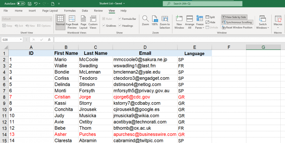
6. As you can see, Excel has highlighted the different cells in “Sheet 2” compared to “Sheet 1”.

How to compare two Excel files — Different cells highlighted

Now you know how to compare two or multiple Excel files and two sheets on your desktop. What if you want to compare and highlight differences in your Excel sheets online?

How to compare two Excel sheets and highlight differences online?

In case you don’t have Excel installed on your desktop or simply prefer to work online altogether, there are online tools that allow you to compare Excel files and sheets for differences.

Below, we provide a list of third-party tools that will allow you to compare Excel files and sheets online:

Layer: Apart from allowing you to review spreadsheet changes and combine multiple spreadsheets into one, Layer offers additional features for file storage and management at a business level.
Synkronizer Excel Compare: In addition to the features outlined in this article, it allows you to combine multiple Excel files into one, while maintaining unique values and avoiding duplicates.
Ablebits Compare Sheets for Excel: This tool provides step-by-step guidance for efficient comparison and displays the differences found between sheets in the “Review Differences” mode for better management.
Florencesoft DiffEngineX: Another excellent alternative that allows you to compare Excel files directly from Microsoft Outlook.

Want to Boost Your Team’s Productivity and Efficiency?

Transform the way your team collaborates with Confluence, a remote-friendly workspace designed to bring knowledge and collaboration together. Say goodbye to scattered information and disjointed communication, and embrace a platform that empowers your team to accomplish more, together.

Key Features and Benefits:

Centralized Knowledge: Access your team’s collective wisdom with ease.
Collaborative Workspace: Foster engagement with flexible project tools.
Seamless Communication: Connect your entire organization effortlessly.
Preserve Ideas: Capture insights without losing them in chats or notifications.
Comprehensive Platform: Manage all content in one organized location.
Open Teamwork: Empower employees to contribute, share, and grow.
Superior Integrations: Sync with tools like Slack, Jira, Trello, and more.

Limited-Time Offer: Sign up for Confluence today and claim your forever-free plan, revolutionizing your team’s collaboration experience.

Conclusion

This article has shown you how to compare the data in two Excel files for differences. You can compare data between two files, two sheets, or multiple files using the side-by-side view for a quick and easy comparison. If your dataset is larger, you can apply the IF formula to compare two Excel sheets or use conditional formatting rules to highlight the differences.

Alternatively, for users that prefer to work online, there are platforms that can help you achieve this level of comparison in an online setting, for example, Layer. We also recommend reading our blog article on How To Combine Multiple Files into One as a great way to complete this data comparison process.

Источник

Need more help?

See Also

Need more help?

Want more options?

Просмотр рядом, чтобы сравнить таблицы.

Сравните 2 книги.

Расположите рядом несколько таблиц Excel.

Сравните два листа в одной книге.

Быстрое выделение значений, которые различаются.

Формула сравнения.

Как произвести сравнение на отдельном листе.

Как сравнить две таблицы при помощи формулы ВПР.

Выделение различий между таблицами цветом.

Сравнение при помощи сводной таблицы.

Сравнение таблиц с помощью Power Query

Как сравнить таблицы при помощи Ultimat Suite для Excel

Как определить различия между двумя листами Excel

Как выделить различия между двумя листами Excel

Compare Two Excel Sheets in Separate Excel Files (Side-by-Side)

Comparing Multiple Sheets in Separate Excel Files (Side-by-Side)

Compare Two Sheets (Side-by-Side) in the Same Excel Workbook

Compare Two Sheets and Highlight Differences (Using Conditional Formatting)

Compare Two Excel Files/Sheets And Get The Differences Using Formula

Compare Two Excel Files/Sheets And Get The Differences Using VBA

Using a Third-Party Tool – XL Comparator

How to compare two Excel files using side-by-side view?

How to Combine Multiple Excel Files Into One

How to compare two Excel sheets using side-by-side view?

How to compare multiple Excel files using side-by-side view?

How to compare two Excel sheets using a formula?

How to compare two Excel sheets using conditional formatting?

How to compare two Excel sheets and highlight differences online?

Want to Boost Your Team’s Productivity and Efficiency?

Conclusion