Excel combining cell text

Combine text from two or more cells into one cell

You can combine data from multiple cells into a single cell using the Ampersand symbol (&) or the CONCAT function.

Combine data with the Ampersand symbol (&)

Select the cell where you want to put the combined data.
Type = and select the first cell you want to combine.
Type & and use quotation marks with a space enclosed.
Select the next cell you want to combine and press enter. An example formula might be =A2&» «&B2.

Combine data using the CONCAT function

Select the cell where you want to put the combined data.
Type =CONCAT(.
Select the cell you want to combine first.

Use commas to separate the cells you are combining and use quotation marks to add spaces, commas, or other text.
Close the formula with a parenthesis and press Enter. An example formula might be =CONCAT(A2, » Family»).

Need more help?

Concatenate is simply a fancy way ot saying “to combine” or “to join together” and there is a special CONCATENATE function in Excel to do this. This function allows you to combine text from different cells into one cell. For example, we have a worksheet containing names and contact information. We want to combine the Last Name and First Name columns in each row into the Full Name column.

To begin, select the first cell that will contain the combined, or concatenated, text. Start typing the function into the cell, starting with an equals sign, as follows.

=CONCATENATE(

Now, we enter the arguments for the CONCATENATE function, which tell the function which cells to combine. We want to combine the first two columns, with the First Name (column B) first and then the Last Name (column A). So, our two arguments for the function will be B2 and A2.

There are two ways you can enter the arguments. First, you can type the cell references, separated by commas, after the opening parenthesis and then add a closing parenthesis at the end:

=CONCATENATE(B2,A2)

You can also click on a cell to enter it into the CONCATENATE function. In our example, after typing the name of the function and the opening parenthesis, we click on the B2 cell, type a comma after B2 in the function, click on the A2 cell, and then type the closing parenthesis after A2 in the function.

Press Enter when you’re done adding the cell references to the function.

Notice that there is no space in between the first and last name. That’s because the CONCATENATE function combines exactly what’s in the arguments you give it and nothing more. There is no space after the first name in B2, so no space was added. If you want to add a space, or any other punctuation or details, you must tell the CONCATENATE function to include it.

To add a space between the first and last names, we add a space as another argument to the function, in between the cell references. To do this, we type a space surrounded by double quotes. Make sure the three arguments are separated by commas.

=CONCATENATE(B2," ",A2)

Press Enter.

That’s better. Now, there is a space between the first and last names.

RELATED: How to Automatically Fill Sequential Data into Excel with the Fill Handle

Now, you’re probably thinking you have to type that function in every cell in the column or manually copy it to each cell in the column. Actually, you don’t. We’ve got another neat trick that will help you quickly copy the CONCATENATE function to the other cells in the column (or row). Select the cell in which you just entered the CONCATENATE function. The small square on the lower-right corner of the selected is called the fill handle. The fill handle allows you to quickly copy and paste content to adjacent cells in the same row or column.

Move your cursor over the fill handle until it turns into a black plus sign and then click and drag it down.

The function you just entered is copied down to the rest of the cells in that column, and the cell references are changed to match the row number for each row.

You can also concatenate text from multiple cells using the ampersand (&) operator. For example, you can enter =B2&" "&A2 to get the same result as =CONCATENATE(B2," ",A2) . There’s no real advantage of using one over the other. although using the ampersand operator results in a shorter entry. However, the CONCATENATE function may be more readable, making it easier to understand what’s happening in the cell.

How to Combine Cells in Excel

In this tutorial, you’ll learn how to Combine Cells in Excel in different scenarios:

How to Combine Cells without Space/Separator in Between.
How to Combine Cells with Space/Separator in Between.
How to Combine Cells with Line Breaks in Between.
How to Combine Cells with Text and Numbers.

How to Combine Cells without Space/Separator

This is the easiest and probably the most used way to combine cells in Excel. For example, suppose you have a data set as shown below:

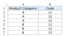
Combine Cells in Excel - Data without separator

You can easily combine cells in columns A and B to get a string such as A11, A12, and so on..

Here is how you can do this:

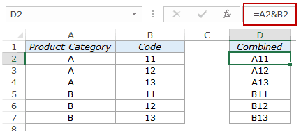
Enter the following formula in a cell where you want the combined string:
```
=A2&B2
```
Copy-paste this in all the cells.

This will give you something as shown below:

Combine Cells in Excel - Result without separator

You can also do the same thing using the CONCATENATE function instead of using the ampersand (&). The below formula would give the same result:

=CONCATENATE(A2,B2)

How to Combine Cells with Space/Separator in Between

You can also combine cells and have a specified separator in between. It could be a space character, a comma, or any other separator.

Suppose we have a dataset as shown below:

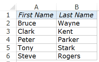
Combine Cells in Excel - Data with separator dataset

Here are the steps to combine the first and the last name with a space character in between:

Enter the following formula in a cell:
```
=A2&" "&B2
```
Copy-paste this in all the cells.

This would combine the first name and last name with a space character in between.

Combine Cells in Excel - Result with separator

If you want any other separator (such as comma, or dot), you can use that in the formula.

How to Combine Cells with Line Breaks in Between

Apart from separators, you can also add line breaks while you combine cells in Excel.

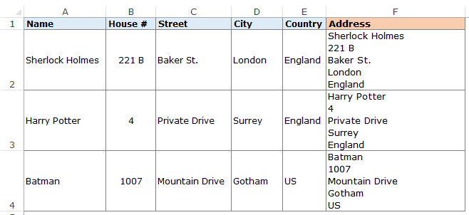
Suppose you have a dataset as shown below:

In the above example, different parts of the address are in different cells (Name, House #, Street, City, and Country).

You can use the CONCATENATE function or the & (ampersand) to combine these cells.

However, just by combining these cells would give you something as shown below:

This is not in a good address format. You can try using the text wrap, but that wouldn’t work either.

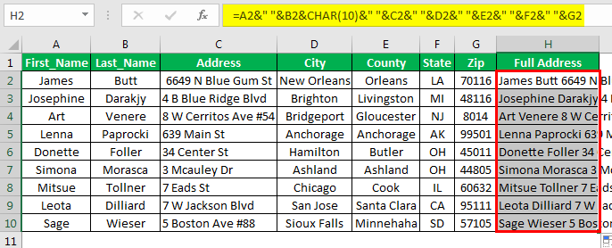
What is needed here is to have each element of the address on a separate line in the same cell. You can achieve that by using the CHAR(10) function along with the & sign.

CHAR(10) is a line feed in Windows, which means that it forces anything after it to go to a new line.

Use the below formula to get each cell’s content on a separate line within the same cell:

=A2&CHAR(10)&B2&CHAR(10)&C2&CHAR(10)&D2&CHAR(10)&E2

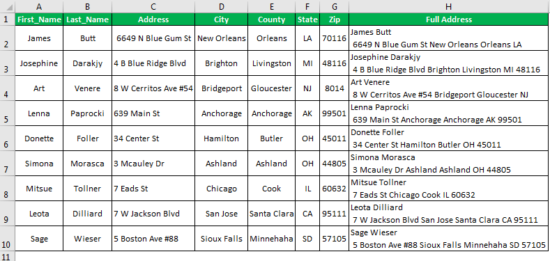
This formula uses the CHAR(10) function in between each cell reference and inserts a line break after each cell. Once you have the result, apply wrap text in the cells that have the results and you’ll get something as shown below:

Combine Cells in Excel - Address with linebreak

How to Combine Cells with Text and Numbers

You can also combine cells that contain different types of data. For example, you can combine cells that contain text and numbers.

Let’s have a look at a simple example first.

Suppose you have a dataset as shown below:

Combine Cells in Excel - text and numbers dataset1

The above data set has text data in one cell and a number is another cell. You can easily combine these two by using the below formula:

=A2&"-"&B2

Here I have used a dash as the separator.

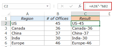
Combine Cells in Excel - text and numbers dash

You can also add some text to it. So you can use the following formula to create a sentence:

=A2&" region has "&B2&" offices"

Here we have used a combination of cell reference and text to construct sentences.

Combine Cells in Excel - text and numbers dash sentence

Now let’s take this example forward and see what happens when you try and use numbers with some formatting applied to it.

Suppose you have a dataset as shown below, where we have sales values.

Combine Cells in Excel - text and numbers sales

Now let’s combine the cells in Column A and B to construct a sentence.

Here the formula I’ll be using:

=A2&" region generated sales of "&B2

Here is how the results look like:

Combine Cells in Excel - text and numbers sales 2

Do you see the problem here? Look closely at the format of the sales value in the result.

Combine Cells in Excel - text and numbers sales 3

You can see that the formatting of the sales value goes away and the result has the plain numeric value. This happens when we combine cells with numbers that have formatting applied to it.

Here is how to fix this. Use the below formula:

=A2&" region generated sales of "&TEXT(B2,"$ ###,0.0")

In the above formula, instead of using B2, we have used the TEXT function. TEXT function makes the number show up in the specified format and as text. In the above case, the format is $ ###,0.0. This format tells Excel to show the number with a dollar sign, a thousand-separator, and one decimal point.

Similarly, you can use the Text function to show in any format allowed in Excel.

Here is another example. There are names and date of birth, and if you try and combine these cells, you get something as shown below:

You can see that Excel completely screws up the date format. The reason is that date and time are stored as numbers in Excel, and when you combine cells that have numbers, as shown above, it shows the number value but doesn’t use the original format.

Here is the formula that will fix this:

=A2&" was born on "&TEXT(B2,"dd mmm yyy")

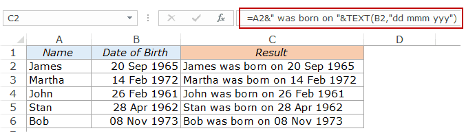
Combine Cells in Excel - DOB with text function

Again, here we have used the TEXT function and specified the format in which we want the Date of Birth to show up in the result.

Here is how this date format works:

dd – Shows the day number of the date. (try using ddd and see what happens).
mmm – shows the three-letter code for a month.
yyy – shows the year number.

Cool… Isn’t it?

Let me know your thoughts in the comments section.

You May Also Like the Following Excel Tutorials:

CONCATENATE Excel Range (with and without separator).
How to Merge Cells in Excel the Right Way.
How to Combine Multiple Workbooks into One Excel Workbook.
How to Combine Data from Multiple Workbooks into One Excel Table (using Power Query).
How to Merge Cells in Excel
How to Combine Duplicate Rows and Sum the Values in Excel
Combine Date and Time in Excel

Источник

We get the data in the cells of the worksheet in Excel, which is how the Excel worksheet works. We can combine multiple cell data, splitting the single-cell data into numerous cells. That is what makes Excel so flexible to use. Combining data from two or more cells into one cell is not the hardest but not the easiest job. It requires very good knowledge of Excel and systematic Excel. This article will show you how to combine text from two or more cells into one cell.

For example, we have a worksheet consisting of product names (column A) and codes (column B). The given product names are A, B, C, and D, and the codes are 2,4,6 and 8, respectively. We need to combine them into one cell (column C). We can easily combine cells in columns A and B by inserting the formula =A2&B2, =A3&B3, and so on to get a string A2, B4, C6, and D8 in column C.

How to Combine Text From Two Or More Cells into One Cell?
- Examples
  - Example #1 – Using the ampersand (&) Symbol
  - Example #2- Combine Cell Reference Values and Manual Values
- Recommended Articles

Examples

Below are examples of combining text from two or more cells into one cell.

You can download this Combine Text to One Cell Excel Template here – Combine Text to One Cell Excel Template

Example #1 – Using the ampersand (&) Symbol

Combine Data to Create a Full Postal Address

While collecting the data from employees, students, or some others, everybody stores the data of full name, last name, address, and additional useful information in parallel columns. Below is a sample of one of those data.

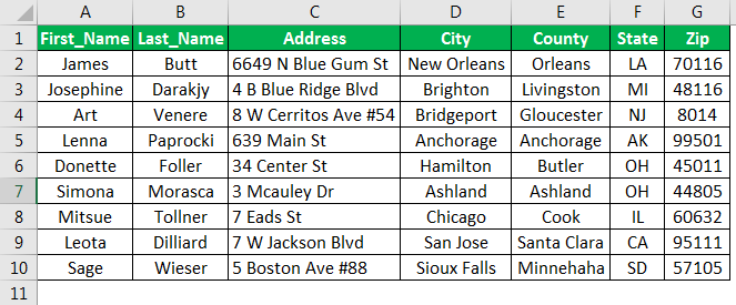
It is fine when collecting the data, but basic and intermediate level Excel users find it difficult when they want to send some post to the respective employee or student because data is scattered into multiple cells.

Usually, when they send the post to the address, they must frame the address like the one below.

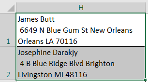
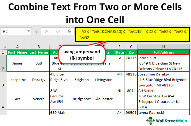
“First Name” and “Last Name” at the top, they need to insert a line breaker, then again they need to combine other address information like “City,” “Country,” “State,” and “Zip Code.” Here, we need the skill to combine text from two or more cells into one cell.

We can combine cells using the built-in Excel function “CONCATENATE Excel functionThe CONCATENATE function in Excel helps the user concatenate or join two or more cell values which may be in the form of characters, strings or numbers.read more” and the ampersand (&) symbol. In this example, we will use only the ampersand symbol.

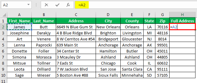
We must copy the above data into the worksheet.

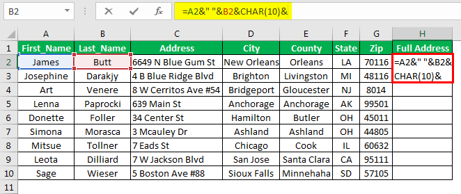
Then, we must open an equal sign in the H2 cell and select the first name cell, i.e., the A2 cell.

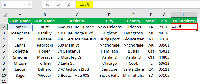
Put the ampersand sign.

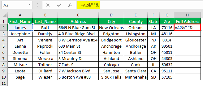
After selecting one value, we need space characters to separate one value from another. So, insert a space character in double quotes.

Now, we must select the second value to be combined, i.e., the last name cell, the B2 cell.

Once the “First Name” and “Last Name” are combined, we need the address in the next line, so we need to insert a line breaker in the same cell.

How do we insert the line breaker is the question now?

We need to make use of the CHAR function in ExcelThe character function in Excel, also known as the char function, identifies the character based on the number or integer accepted by the computer language. For example, the number for character «A» is 65, so if we use =char(65), we get A.read more. Using the number 10 in the CHAR function, we will insert a line breaker. So, we will use CHAR(10).

Now, we must select “Address” and give the space character.

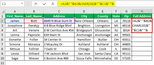
Similarly, we must select other cells and give each cell a one-space character.

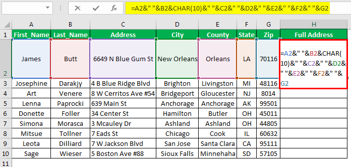
Now, we can see the full address in one cell.

Next, we will copy and paste the formula to the below cells.

But we cannot see any line breaker here.

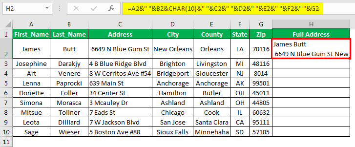
Once the formula is applied, we need to apply the Wrap TextWrap text in Excel belongs to the “Formatting” class of excel function that does not make any changes to the value of the cell but just change the way a sentence is displayed in the cell. This means that a sentence that is formatted as warp text is always the same as that sentence that is not formatted as a wrap text.read more format to the formula cell.

As a result, it will make the proper address format.

Example #2- Combine Cell Reference Values and Manual Values

Not only cell references, but we can also include our values with cell referencesCell reference in excel is referring the other cells to a cell to use its values or properties. For instance, if we have data in cell A2 and want to use that in cell A1, use =A2 in cell A1, and this will copy the A2 value in A1.read more. For example, look at the below data.

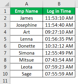
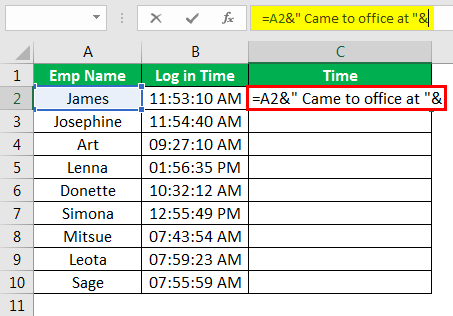
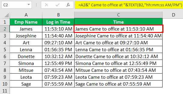
We need to combine the above two columns of data into one with the manual word “came to office at,” and the full sentence should read like the one below.

Example: “James came to the office at 11:53:10 AM.”

Let us copy the above data to Excel and open an equal sign in cell C2. Then, the first value to be combined is cell A2.

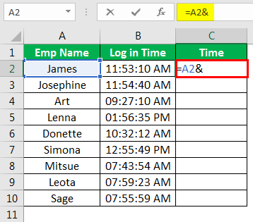
Next, we need our manual value. So, we must insert the manual value in double quotes.

Then, we must select the final value, the “Time” cell.

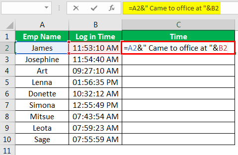
As a result, we can see the full sentences.

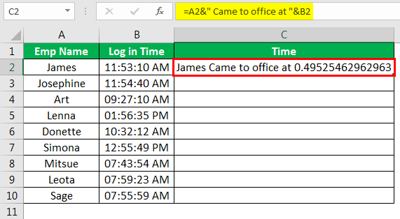
Then, we must copy and paste the formula into other cells.

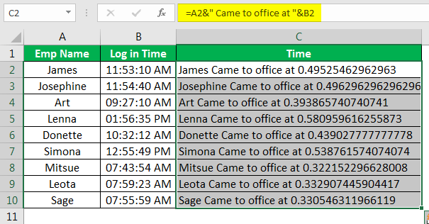
We have one problem here, i.e., the time portion is not properly appearing. The reason why we cannot see proper time is that Excel stores time in decimal serial numbers. Therefore, whenever we combine time with other cells, we need to connect them with proper formatting.

To apply the time format, we need to use TEXT Formula in Excel with the format “hh:mm:ss AM/PM.”

By using different techniques, we can combine text from two or more cells into one cell.

Combine text using Ampersand symbol

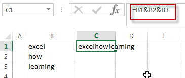
If you want to combine text from multiple cells into one cell and you can use the Ampersand (&) symbol. For example, if you want to combine texts in the Range B1:B3 into Cell C1, Just refer to the following steps:

1# Click Cell C1 that you want to put the combined text.

2# type the below formula in the formula box of C1.

=B1&B2&B3

3# press Enter, you will see that the text content in B1:B3 will be joined into C1.

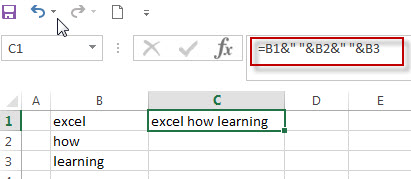
Note:

If you want to add a space between the combined text, then you can use &” ” & instead of & in the above formula.

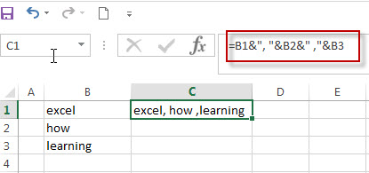
And if you want to add a comma to the combined text, just type &”,”& between the combined cells in the above formula.

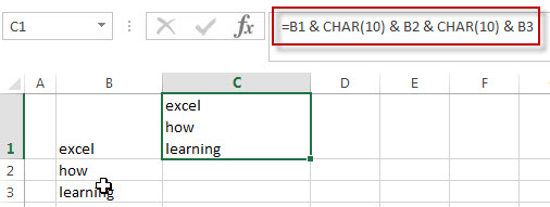
If you want to add Line break between the combined cells using Ampersand operator, you should combine with the CHAR function to get the line break. Using the following formula:

=B1 & CHAR(10) & B2 & CHAR(10) & B3

Combine text using CONCATENATE function

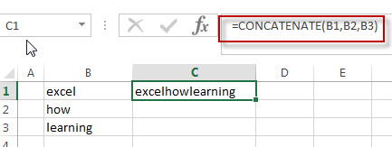
If you want to join the text from multiple cells into one cell, you also can use the CONCATENATE function instead of Ampersand operator. Just following the below steps to join combine the text from B1:B3 into one Cell C1.

1# Select the cell in which you want to put the combined text. (Select Cell C1)

2# type the following formula in Cell C1.

=CONCATENATE(B1,B2,B3)

3# press Enter to complete the formula.

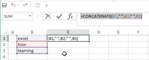
Note: If you want to add a space between the combined text strings, you can add a space character (“ “) enclosed in quotation marks. Just like the below formula:

=CONCATENATE(B1," ",B2," ",B3)

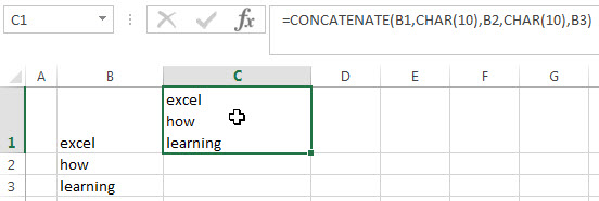
If you want to add line break into the combined text string, you can use the CHAR function within the CONCATENATE function, just use the below formula:

=CONCATENATE(B1,CHAR(10),B2,CHAR(10),B3)

Combine text using TEXTJOIN function

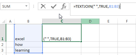
If you are using the excel 2016, then you can use a new function TEXTJOIN function to combine text from multiple cells, it is only available in EXCEL 2016. It can join the text from two or more text strings or multiple ranges into one string and also can specify a delimiter between the combined text strings. Just like the below formula:

=TEXTJOIN(" ",TRUE,B1:B3)

Remove Numeric Characters from a Cell
If you want to remove numeric characters from alphanumeric string, you can use the following complex array formula using a combination of the TEXTJOIN function, the MID function, the Row function, and the INDIRECT function..…
remove non numeric characters from a cell
If you want to remove non numeric characters from a text cell in excel, you can use the array formula:{=TEXTJOIN(“”,TRUE,IFERROR(MID(B1,ROW(INDIRECT(“1:”&LEN(B1))),1)+0,””))}…

Excel Concat function
The excel CONCAT function combines 2 or more strings or ranges together.This is a new function in Excel 2016 and it replaces the CONCATENATE function.The syntax of the CONCAT function is as below:=CONCAT (text1,[text2],…)…
Excel CHAR function
The Excel CHAR function returns the character specified by a number (ASCII Value).The CHAR function is a build-in function in Microsoft Excel and it is categorized as a Text Function. The syntax of the CHAR function is as below:=CHAR(number)….
Excel TEXTJOIN function
The Excel TEXTJOIN function joins two or more text strings together and separated by a delimiter. you can select an entire range of cell references to be combined in excel 2016.The syntax of the TEXTJOIN function is as below:= TEXTJOIN (delimiter, ignore_empty,text1,[text2])…

Источник

Combine text from two or more cells into one cell

Combine data with the Ampersand symbol (&)

Combine data using the CONCAT function

Need more help?

See also

Need more help?

How to Combine Cells in Excel

How to Combine Cells without Space/Separator

How to Combine Cells with Space/Separator in Between

How to Combine Cells with Line Breaks in Between

How to Combine Cells with Text and Numbers

Table of contents

Examples

Example #1 – Using the ampersand (&) Symbol

Example #2- Combine Cell Reference Values and Manual Values

Recommended Articles

Combine text using Ampersand symbol

Combine text using CONCATENATE function

Combine text using TEXTJOIN function