Excel combine cells as text

Combine text from two or more cells into one cell

You can combine data from multiple cells into a single cell using the Ampersand symbol (&) or the CONCAT function.

Combine data with the Ampersand symbol (&)

1. Select the cell where you want to put the combined data.

2. Type = and select the first cell you want to combine.

3. Type & and use quotation marks with a space enclosed.

4. Select the next cell you want to combine and press enter. An example formula might be =A2&» «&B2.

Combine data using the CONCAT function

1. Select the cell where you want to put the combined data.

2. Type =CONCAT(.

3. Select the cell you want to combine first.

   Use commas to separate the cells you are combining and use quotation marks to add spaces, commas, or other text.

4. Close the formula with a parenthesis and press Enter. An example formula might be =CONCAT(A2, » Family»).

Need more help?

See also

TEXTJOIN function

CONCAT function

Merge and unmerge cells

CONCATENATE function

How to avoid broken formulas

Automatically number rows

Watch Video – Combine cells in Excel (using Formulas)

A lot of times, we need to work with text data in Excel. It could be Names, Address, Email ids, or other kinds of text strings. Often, there is a need to combine cells in Excel that contain the text data.

Your data could be in adjacent cells (rows/columns), or it could be far off in the same worksheet or even a different worksheet.

How to Combine Cells in Excel

In this tutorial, you’ll learn how to Combine Cells in Excel in different scenarios:

• How to Combine Cells without Space/Separator in Between.
• How to Combine Cells with Space/Separator in Between.
• How to Combine Cells with Line Breaks in Between.
• How to Combine Cells with Text and Numbers.

How to Combine Cells without Space/Separator

This is the easiest and probably the most used way to combine cells in Excel. For example, suppose you have a data set as shown below:

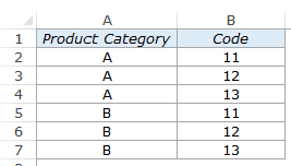
You can easily combine cells in columns A and B to get a string such as A11, A12, and so on..

Here is how you can do this:

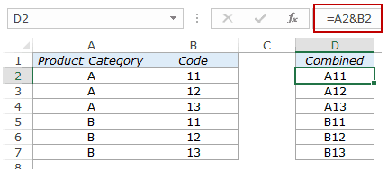
• Enter the following formula in a cell where you want the combined string:

  =A2&B2

• Copy-paste this in all the cells.

This will give you something as shown below:

You can also do the same thing using the CONCATENATE function instead of using the ampersand (&). The below formula would give the same result:

=CONCATENATE(A2,B2)

How to Combine Cells with Space/Separator in Between

You can also combine cells and have a specified separator in between. It could be a space character, a comma, or any other separator.

Suppose we have a dataset as shown below:

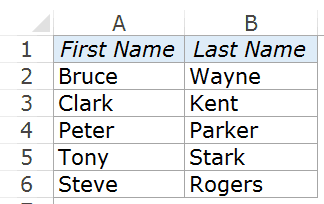
Here are the steps to combine the first and the last name with a space character in between:

• Enter the following formula in a cell:

  =A2&" "&B2

• Copy-paste this in all the cells.

This would combine the first name and last name with a space character in between.

If you want any other separator (such as comma, or dot), you can use that in the formula.

How to Combine Cells with Line Breaks in Between

Apart from separators, you can also add line breaks while you combine cells in Excel.

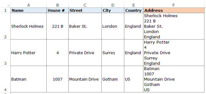
Suppose you have a dataset as shown below:

In the above example, different parts of the address are in different cells (Name, House #, Street, City, and Country).

You can use the CONCATENATE function or the & (ampersand) to combine these cells.

However, just by combining these cells would give you something as shown below:

This is not in a good address format. You can try using the text wrap, but that wouldn’t work either.

What is needed here is to have each element of the address on a separate line in the same cell. You can achieve that by using the CHAR(10) function along with the & sign.

CHAR(10) is a line feed in Windows, which means that it forces anything after it to go to a new line.

Use the below formula to get each cell’s content on a separate line within the same cell:

=A2&CHAR(10)&B2&CHAR(10)&C2&CHAR(10)&D2&CHAR(10)&E2

This formula uses the CHAR(10) function in between each cell reference and inserts a line break after each cell. Once you have the result, apply wrap text in the cells that have the results and you’ll get something as shown below:

How to Combine Cells with Text and Numbers

You can also combine cells that contain different types of data. For example, you can combine cells that contain text and numbers.

Let’s have a look at a simple example first.

Suppose you have a dataset as shown below:

The above data set has text data in one cell and a number is another cell. You can easily combine these two by using the below formula:

=A2&"-"&B2

Here I have used a dash as the separator.

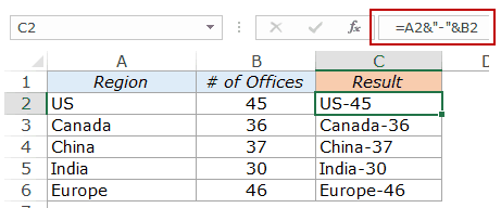
You can also add some text to it. So you can use the following formula to create a sentence:

=A2&" region has "&B2&" offices"

Here we have used a combination of cell reference and text to construct sentences.

Now let’s take this example forward and see what happens when you try and use numbers with some formatting applied to it.

Suppose you have a dataset as shown below, where we have sales values.

Now let’s combine the cells in Column A and B to construct a sentence.

Here the formula I’ll be using:

=A2&" region generated sales of "&B2

Here is how the results look like:

Do you see the problem here? Look closely at the format of the sales value in the result.

You can see that the formatting of the sales value goes away and the result has the plain numeric value. This happens when we combine cells with numbers that have formatting applied to it.

Here is how to fix this. Use the below formula:

=A2&" region generated sales of "&TEXT(B2,"$ ###,0.0")

In the above formula, instead of using B2, we have used the TEXT function. TEXT function makes the number show up in the specified format and as text. In the above case, the format is $ ###,0.0. This format tells Excel to show the number with a dollar sign, a thousand-separator, and one decimal point.

Similarly, you can use the Text function to show in any format allowed in Excel.

Here is another example. There are names and date of birth, and if you try and combine these cells, you get something as shown below:

You can see that Excel completely screws up the date format. The reason is that date and time are stored as numbers in Excel, and when you combine cells that have numbers, as shown above, it shows the number value but doesn’t use the original format.

Here is the formula that will fix this:

=A2&" was born on "&TEXT(B2,"dd mmm yyy")

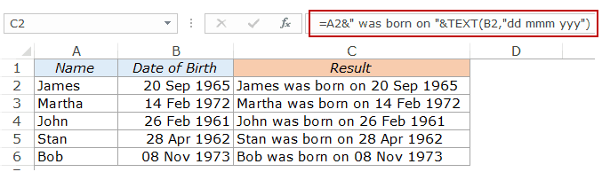
Again, here we have used the TEXT function and specified the format in which we want the Date of Birth to show up in the result.

Here is how this date format works:

• dd – Shows the day number of the date. (try using ddd and see what happens).
• mmm – shows the three-letter code for a month.
• yyy – shows the year number.

Cool… Isn’t it?

Let me know your thoughts in the comments section.

You May Also Like the Following Excel Tutorials:

• CONCATENATE Excel Range (with and without separator).
• How to Merge Cells in Excel the Right Way.
• How to Combine Multiple Workbooks into One Excel Workbook.
• How to Combine Data from Multiple Workbooks into One Excel Table (using Power Query).
• How to Merge Cells in Excel
• How to Combine Duplicate Rows and Sum the Values in Excel
• Combine Date and Time in Excel

If you have a large worksheet in an Excel workbook in which you need to combine text from multiple cells, you can breathe a sigh of relief because you don’t have to retype all that text. You can easily concatenate the text.

Concatenate is simply a fancy way ot saying “to combine” or “to join together” and there is a special CONCATENATE function in Excel to do this. This function allows you to combine text from different cells into one cell. For example, we have a worksheet containing names and contact information. We want to combine the Last Name and First Name columns in each row into the Full Name column.

To begin, select the first cell that will contain the combined, or concatenated, text. Start typing the function into the cell, starting with an equals sign, as follows.

=CONCATENATE(

Now, we enter the arguments for the CONCATENATE function, which tell the function which cells to combine. We want to combine the first two columns, with the First Name (column B) first and then the Last Name (column A). So, our two arguments for the function will be B2 and A2.

There are two ways you can enter the arguments. First, you can type the cell references, separated by commas, after the opening parenthesis and then add a closing parenthesis at the end:

=CONCATENATE(B2,A2)

You can also click on a cell to enter it into the CONCATENATE function. In our example, after typing the name of the function and the opening parenthesis, we click on the B2 cell, type a comma after B2 in the function, click on the A2 cell, and then type the closing parenthesis after A2 in the function.

Press Enter when you’re done adding the cell references to the function.

Notice that there is no space in between the first and last name. That’s because the CONCATENATE function combines exactly what’s in the arguments you give it and nothing more. There is no space after the first name in B2, so no space was added. If you want to add a space, or any other punctuation or details, you must tell the CONCATENATE function to include it.

To add a space between the first and last names, we add a space as another argument to the function, in between the cell references. To do this, we type a space surrounded by double quotes. Make sure the three arguments are separated by commas.

=CONCATENATE(B2," ",A2)

Press Enter.

That’s better. Now, there is a space between the first and last names.

RELATED: How to Automatically Fill Sequential Data into Excel with the Fill Handle

Now, you’re probably thinking you have to type that function in every cell in the column or manually copy it to each cell in the column. Actually, you don’t. We’ve got another neat trick that will help you quickly copy the CONCATENATE function to the other cells in the column (or row). Select the cell in which you just entered the CONCATENATE function. The small square on the lower-right corner of the selected is called the fill handle. The fill handle allows you to quickly copy and paste content to adjacent cells in the same row or column.

Move your cursor over the fill handle until it turns into a black plus sign and then click and drag it down.

The function you just entered is copied down to the rest of the cells in that column, and the cell references are changed to match the row number for each row.

You can also concatenate text from multiple cells using the ampersand (&) operator. For example, you can enter =B2&" "&A2 to get the same result as =CONCATENATE(B2," ",A2) . There’s no real advantage of using one over the other. although using the ampersand operator results in a shorter entry. However, the CONCATENATE function may be more readable, making it easier to understand what’s happening in the cell.

READ NEXT

• › How to Merge Two Columns in Microsoft Excel
• › 12 Basic Excel Functions Everybody Should Know
• › How to Combine Data From Spreadsheets in Microsoft Excel
• › 9 Useful Microsoft Excel Functions for Working With Text
• › How to Calculate Age in Microsoft Excel
• › How to Concatenate in Microsoft Excel
• › The Basics of Structuring Formulas in Microsoft Excel
• › BLUETTI Slashed Hundreds off Its Best Power Stations for Easter Sale

Combining values with CONCATENATE is the best way, but with this function, it’s not possible to refer to an entire range.

You need to select all the cells of a range one by one, and if you try to refer to an entire range, it will return the text from the first cell.

In this situation, you do need a method where you can refer to an entire range of cells to combine them in a single cell.

So today in this post, I’d like to share with you 5 different ways to combine text from a range into a single cell.

[CONCATENATE + TRANSPOSE] to Combine Values

The best way to combine text from different cells into one cell is by using the transpose function with concatenating function.

Look at the below range of cells where you have a text but every word is in a different cell and you want to get it all in one cell.

Below are the steps you need to follow to combine values from this range of cells into one cell.

1. In the B8 (edit the cell using F2), insert the following formula, and do not press enter.
   • =CONCATENATE(TRANSPOSE(A1:A5)&” “)
2. Now, select the entire inside portion of the concatenate function and press F9. It will convert it into an array.
3. After that, remove the curly brackets from the start and the end of the array.
4. In the end, hit enter.

That’s all.

How this formula works

In this formula, you have used TRANSPOSE and space in the CONCATENATE. When you convert that reference into hard values it returns an array.

In this array, you have the text from each cell and a space between them and when you hit enter, it combines all of them.

Combine Text using the Fill Justify Option

Fill justify is one of the unused but most powerful tools in Excel. And, whenever you need to combine text from different cells you can use it.

The best thing is, that you need a single click to merge text. Have look at the below data and follow the steps.

1. First of all, make sure to increase the width of the column where you have text.
2. After that, select all the cells.
3. In the end, go to Home Tab ➜ Editing ➜ Fill ➜ Justify.

This will merge text from all the cells into the first cell of the selection.

TEXTJOIN Function for CONCATENATE Values

If you are using Excel 2016 (Office 365), there is a function called “TextJoin”. It can make it easy for you to combine text from different cells into a single cell.

Syntax:

TEXTJOIN(delimiter, ignore_empty, text1, [text2], …)

1. delimiter a text string to use as a delimiter.
2. ignore_empty true to ignore blank cell, false to not.
3. text1 text to combine.
4. [text2] text to combine optional.

how to use it

To combine the below list of values you can use the formula:

=TEXTJOIN(" ",TRUE,A1:A5)

Here you have used space as a delimiter, TRUE to ignore blank cells and the entire range in a single argument. In the end, hit enter and you’ll get all the text in a single cell.

Combine Text with Power Query

Power Query is a fantastic tool and I love it. Make sure to check out this (Excel Power Query Tutorial). You can also use it to combine text from a list in a single cell. Below are the steps.

1. Select the range of cells and click on “From table” in data tab.
   
2. If will edit your data into Power Query editor.
   
3. Now from here, select the column and go to “Transform Tab”.
4. From “Transform” tab, go to Table and click on “Transpose”.
   
5. For this, select all the columns (select first column, press and hold shift key, click on the last column) and press right click and then select “Merge”.
   
6. After that, from Merge window, select space as a separator and name the column.
   
7. In the end, click OK and click on “Close and Load”.

Now you have a new worksheet in your workbook with all the text in a single cell. The best thing about using Power Query is you don’t need to do this setup again and again.

When you update the old list with a new value you need to refresh your query and it will add that new value to the cell.

VBA Code to Combine Values

If you want to use a macro code to combine text from different cells then I have something for you. With this code, you can combine text in no time. All you need to do is, select the range of cells where you have the text and run this code.

 Sub combineText()
 Dim rng As Range
 Dim i As String
 For Each rng In Selection
 i = i & rng & " "
 Next rng
 Range("B1").Value = Trim(i)
 End Sub 

Make sure to specify your desired location in the code where you want to combine the text.

In the end,

There may be different situations for you where you need to concatenate a range of cells into a single cell. And that’s why we have these different methods.

All methods are easy and quick, you need to select the right method as per your need. I must say that give a try to all the methods once and tell me:

Which one is your favorite and worked for you?

Please share your views with me in the comment section. I’d love to hear from you, and please, don’t forget to share this post with your friends, I am sure they will appreciate it.

Надпись на заборе: «Катя + Миша + Семён + Юра + Дмитрий Васильевич +
товарищ Никитин + рыжий сантехник + Витенька + телемастер Жора +
сволочь Редулов + не вспомнить имени, длинноволосый такой +
ещё 19 мужиков + муж = любовь!»

Способ 1. Функции СЦЕПИТЬ, СЦЕП и ОБЪЕДИНИТЬ

В категории Текстовые есть функция СЦЕПИТЬ (CONCATENATE), которая соединяет содержимое нескольких ячеек (до 255) в одно целое, позволяя комбинировать их с произвольным текстом. Например, вот так:

Нюанс: не забудьте о пробелах между словами — их надо прописывать как отдельные аргументы и заключать в скобки, ибо текст. 

Очевидно, что если нужно собрать много фрагментов, то использовать эту функцию уже не очень удобно, т.к. придется прописывать ссылки на каждую ячейку-фрагмент по отдельности. Поэтому, начиная с 2016 версии Excel, на замену функции СЦЕПИТЬ пришла ее более совершенная версия с похожим названием и тем же синтаксисом — функция СЦЕП (CONCAT). Ее принципиальное отличие в том, что теперь в качестве аргументов можно задавать не одиночные ячейки, а целые диапазоны — текст из всех ячеек всех диапазонов будет объединен в одно целое:

Для массового объединения также удобно использовать новую функцию ОБЪЕДИНИТЬ (TEXTJOIN), появившуюся начиная с Excel 2016. У нее следующий синтаксис:

=ОБЪЕДИНИТЬ(Разделитель; Пропускать_ли_пустые_ячейки; Диапазон1; Диапазон2 … )

где

• Разделитель — символ, который будет вставлен между фрагментами
• Второй аргумент отвечает за то, нужно ли игнорировать пустые ячейки (ИСТИНА или ЛОЖЬ)
• Диапазон 1, 2, 3 … — диапазоны ячеек, содержимое которых хотим склеить

Например:

Способ 2. Символ для склеивания текста (&)

Это универсальный и компактный способ сцепки, работающий абсолютно во всех версиях Excel. 

Для суммирования содержимого нескольких ячеек используют знак плюс «+«, а для склеивания содержимого ячеек используют знак «&» (расположен на большинстве клавиатур на цифре «7»). При его использовании необходимо помнить, что:

• Этот символ надо ставить в каждой точке соединения, т.е. на всех «стыках» текстовых строк также, как вы ставите несколько плюсов при сложении нескольких чисел (2+8+6+4+8)
• Если нужно приклеить произвольный текст (даже если это всего лишь точка или пробел, не говоря уж о целом слове), то этот текст надо заключать в кавычки. В предыдущем примере с функцией СЦЕПИТЬ о кавычках заботится сам Excel — в этом же случае их надо ставить вручную.

Вот, например, как можно собрать ФИО в одну ячейку из трех с добавлением пробелов:

Если сочетать это с функцией извлечения из текста первых букв — ЛЕВСИМВ (LEFT), то можно получить фамилию с инициалами одной формулой:

Способ 3. Макрос для объединения ячеек без потери текста.

Имеем текст в нескольких ячейках и желание — объединить эти ячейки в одну, слив туда же их текст. Проблема в одном — кнопка Объединить и поместить в центре (Merge and Center) в Excel объединять-то ячейки умеет, а вот с текстом сложность — в живых остается только текст из верхней левой ячейки. 

Чтобы объединение ячеек происходило с объединением текста (как в таблицах Word) придется использовать макрос. Для этого откройте редактор Visual Basic  на вкладке Разработчик — Visual Basic (Developer — Visual Basic) или сочетанием клавиш Alt+F11, вставим в нашу книгу новый программный модуль (меню Insert — Module) и скопируем туда текст такого простого макроса:

Sub MergeToOneCell()
    Const sDELIM As String = " "     'символ-разделитель
    Dim rCell As Range
    Dim sMergeStr As String
    If TypeName(Selection) <> "Range" Then Exit Sub   'если выделены не ячейки - выходим
    With Selection
        For Each rCell In .Cells
            sMergeStr = sMergeStr & sDELIM & rCell.Text  'собираем текст из ячеек
        Next rCell
        Application.DisplayAlerts = False   'отключаем стандартное предупреждение о потере текста
        .Merge Across:=False                'объединяем ячейки
        Application.DisplayAlerts = True
        .Item(1).Value = Mid(sMergeStr, 1 + Len(sDELIM))    'добавляем к объед.ячейке суммарный текст
    End With
End Sub

Теперь, если выделить несколько ячеек и запустить этот макрос с помощью сочетания клавиш Alt+F8 или кнопкой Макросы на вкладке Разработчик (Developer — Macros), то Excel объединит выделенные ячейки в одну, слив туда же и текст через пробелы.

Ссылки по теме

• Делим текст на куски
• Объединение нескольких ячеек в одну с сохранением текста с помощью надстройки PLEX
• Что такое макросы, как их использовать, куда вставлять код макроса на VBA