
Excel for Microsoft 365 for Mac Excel 2021 for Mac Excel 2019 for Mac Excel 2016 for Mac Excel for Mac 2011 More…Less
Cause: The default cell reference style (A1), which refers to columns as letters and refers to rows as numbers, was changed.
Solution: Clear the R1C1 reference style selection in Excel preferences.
Difference between A1 and R1C1 reference styles
-
On the Excel menu, click Preferences.
-
Under Authoring, click Calculation
 .
. -
Clear the Use R1C1 reference style check box.
The column headings now show A, B, and C, instead of 1, 2, 3, and so on.
 .
.Need more help?

This Excel tutorial explains how to change column headings from numbers (1, 2, 3, 4) back to letters (A, B, C, D) in Excel 2016 (with screenshots and step-by-step instructions).
Question: In Microsoft Excel 2016, my Excel spreadsheet has numbers for both rows and columns. How do I change the column headings back to letters such as A, B, C, D?
Answer: Traditionally, column headings are represented by letters such as A, B, C, D. If your spreadsheet shows the columns as numbers, you can change the headings back to letters with a few easy steps.
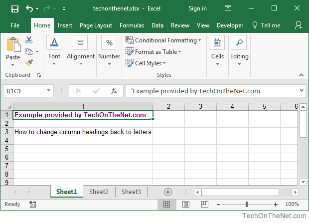
In the example below, the column headings are numbered 1, 2, 3, 4 instead of the traditional A, B, C, D values that you normally see in Excel. When the column headings are numeric values, R1C1 reference style is being displayed in the spreadsheet.
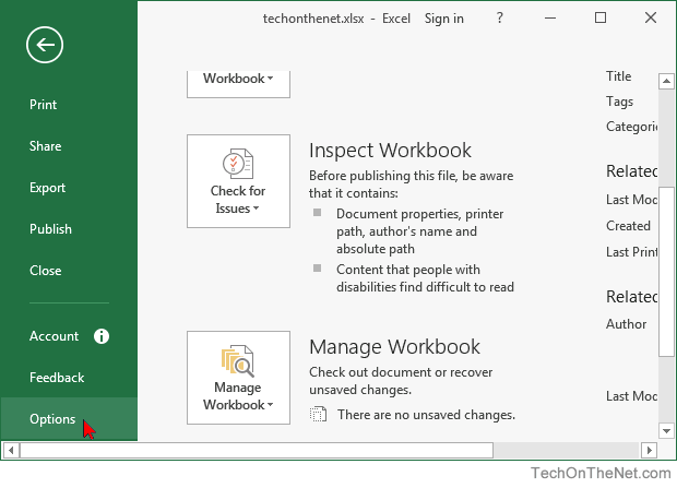
To change the column headings to letters, select the File tab in the toolbar at the top of the screen and then click on Options at the bottom of the menu.
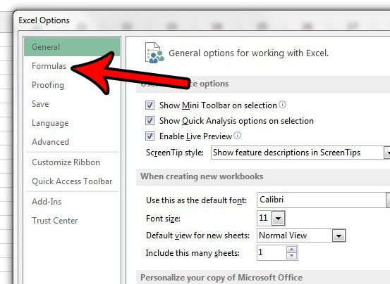
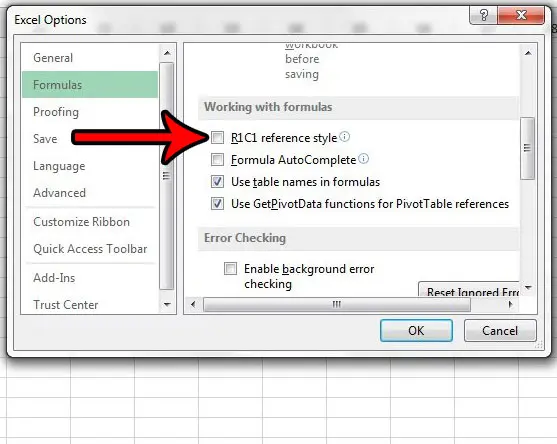
When the Excel Options window appears, click on the Formulas option on the left. Then uncheck the option called «R1C1 reference style» and click on the OK button.

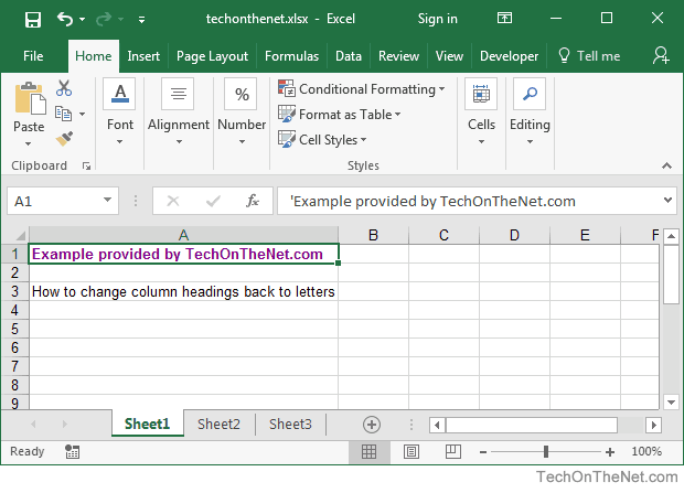
Now when you return to your spreadsheet, the column headings should be letters (A, B, C, D) instead of numbers (1, 2, 3, 4).
Skip to content
![]()
Excel has an option for showing column letters instead of number. This can be useful, for example, when you work with VBA macros or when you have to count columns (e.g. VLOOKUP). But in most cases, you would prefer letters. In this article we learn how to change column numbers to letters and the other way around in Excel.
Effect of numbers instead of letters in column headings
If you see numbers instead of letters for the column headings, you will also notice the following effect: All cell references are replaced by numbers. This style is called R1C1 reference style.
Instead of ‘=$A$2’, you will find ‘=R1C2’ for row 1 and column 2. If we remove the dollar signs, this formula might look completely different as it will always show the distance from the current cell.
Steps for changing from column letters to numbers
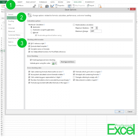
You can switch from column letters to numbers quite easily in Excel (the following numbers are referring to the picture above):
- Go To File and click on Options.
- Select Formulas on the left hand side.
- Tick “R1C1 reference style”.
Switching back from numbers to letters works the same way. Only in the last step, you have to remove the tick from “R1C1 reference style”.
Please note that all references within formulas will be replaced by numbers.

Henrik Schiffner is a freelance business consultant and software developer. He lives and works in Hamburg, Germany. Besides being an Excel enthusiast he loves photography and sports.
We use cookies on our website to give you the most relevant experience by remembering your preferences and repeat visits. By clicking “Accept”, you consent to the use of ALL the cookies.
.
Have you ever opened an Excel workbook and found that the column headings show numbers instead of letters? The formula look strange too, showing references like RC[-1] instead of D2.

This is R1C1 reference style — a handy feature, and I use it sometimes when programming or setting up a workbook.
Numbers on the column headings make it easier to set up formulas that need a column number, such as VLOOKUP. I don’t have to get fingerprints on my screen, as I count across to column R, where the lookup value is.
Video: Change Excel Column Headings from Numbers to Letters
To see why this happens, and how to switch the column headings back to letters, watch this short video tutorial. The written instructions are below the video.
Your browser can’t show this frame. Here is a link to the page
Why It Happens
Maybe you’ve never heard of R1C1 reference style, and certainly didn’t change any settings. If you didn’t turn that option on, why did the numbers suddenly appear? Probably because someone sent you a workbook, and that’s the first Excel file that you opened today.
The first workbook that you open, when opening Excel, sets the reference style. For example, perhaps I built a workbook for you, and saved it while I was using R1C1 reference style.
I sent you the workbook overnight, and it was the first thing you opened this morning. Surprise! There are numbers in the column headings.
Turn R1C1 Reference Style On or Off
If you close Excel, then open a workbook that you created yourself, with letters in the column headings, that will change the reference style back to A1, which has letters in the column headings.
Or, to manually change the reference style, you can change the option setting.
In Excel 2010:
- At the left end of the Ribbon, click the File tab, then click Options.
- Click the Formulas category.
- In the Working with Formulas section, add or remove the check mark from ‘R1C1 reference style’
- Click OK to close the Options window.

In Excel 2007:
-
- At the left end of the Ribbon, click the Office Button, then click Excel Options.
- Click the Formulas category.
- In the Working with Formulas section, add or remove the check mark from ‘R1C1 reference style’
- Click OK to close the Options window.
In Excel 2003 and earlier versions:
- On the Tools menu, click Options and select the General tab.
- Add or remove the check mark from ‘R1C1 reference style’
- Click OK to close the Options dialog box.

Use a Macro to Switch Headings
If you frequently change the headings from numbers to letters, or letters to numbers, you can create a macro to do the work for you.
There are instructions in this blog post: Excel VBA: Switch Column Headings to Numbers
________________________
Содержание
- Columns and rows are labeled numerically in Excel
- Symptoms
- Cause
- Resolution
- More information
- A1 Reference Style vs. R1C1 Reference Style
- The A1 Reference Style
- The R1C1 Reference Style
- References
- Automatically number rows
- What do you want to do?
- Fill a column with a series of numbers
- Use the ROW function to number rows
- Display or hide the fill handle
- Столбцы и строки помечены как число в Excel
- Симптомы
- Причина
- Решение
- Дополнительные сведения
- Стиль ссылок A1 и стиль ссылок R1C1
- Стиль ссылки A1
- Стиль ссылки R1C1
- Ссылки
- How to number columns in Excel and convert column letter to number
- How to return column number in Excel
- How to convert column letter to number (non-volatile formula)
- Change column letter to number using a custom function
- Return column number of a specific cell
- Get column letter of the current cell
- How to show column numbers in Excel
- How to number columns in Excel
Columns and rows are labeled numerically in Excel
Symptoms
Your column labels are numeric rather than alphabetic. For example, instead of seeing A, B, and C at the top of your worksheet columns, you see 1, 2, 3, and so on.
Cause
This behavior occurs when the R1C1 reference style check box is selected in the Options dialog box.
Resolution
To change this behavior, follow these steps:
- Start Microsoft Excel.
- On the Tools menu, click Options.
- Click the Formulas tab.
- Under Working with formulas, click to clear the R1C1 reference style check box (upper-left corner), and then click OK.
If you select the R1C1 reference style check box, Excel changes the reference style of both row and column headings, and cell references from the A1 style to the R1C1 style.
More information
A1 Reference Style vs. R1C1 Reference Style
The A1 Reference Style
By default, Excel uses the A1 reference style, which refers to columns as letters (A through IV, for a total of 256 columns), and refers to rows as numbers (1 through 65,536). These letters and numbers are called row and column headings. To refer to a cell, type the column letter followed by the row number. For example, D50 refers to the cell at the intersection of column D and row 50. To refer to a range of cells, type the reference for the cell that is in the upper-left corner of the range, type a colon (:), and then type the reference to the cell that is in the lower-right corner of the range.
The R1C1 Reference Style
Excel can also use the R1C1 reference style, in which both the rows and the columns on the worksheet are numbered. The R1C1 reference style is useful if you want to compute row and column positions in macros. In the R1C1 style, Excel indicates the location of a cell with an «R» followed by a row number and a «C» followed by a column number.
References
For more information about this topic, click Microsoft Excel Help on the Help menu, type about cell and range references in the Office Assistant or the Answer Wizard, and then click Search to view the topic.
Источник
Automatically number rows
Unlike other Microsoft 365 programs, Excel does not provide a button to number data automatically. But, you can easily add sequential numbers to rows of data by dragging the fill handle to fill a column with a series of numbers or by using the ROW function.
Tip: If you are looking for a more advanced auto-numbering system for your data, and Access is installed on your computer, you can import the Excel data to an Access database. In an Access database, you can create a field that automatically generates a unique number when you enter a new record in a table.

What do you want to do?
Fill a column with a series of numbers
Select the first cell in the range that you want to fill.
Type the starting value for the series.
Type a value in the next cell to establish a pattern.
Tip: For example, if you want the series 1, 2, 3, 4, 5. type 1 and 2 in the first two cells. If you want the series 2, 4, 6, 8. type 2 and 4.
Select the cells that contain the starting values.
Note: In Excel 2013 and later, the Quick Analysis button is displayed by default when you select more than one cell containing data. You can ignore the button to complete this procedure.
Drag the fill handle  across the range that you want to fill.
Note: As you drag the fill handle across each cell, Excel displays a preview of the value. If you want a different pattern, drag the fill handle by holding down the right-click button, and then choose a pattern.
To fill in increasing order, drag down or to the right. To fill in decreasing order, drag up or to the left.
Tip: If you do not see the fill handle, you may have to display it first. For more information, see Display or hide the fill handle.
Note: These numbers are not automatically updated when you add, move, or remove rows. You can manually update the sequential numbering by selecting two numbers that are in the right sequence, and then dragging the fill handle to the end of the numbered range.
Use the ROW function to number rows
In the first cell of the range that you want to number, type =ROW(A1).
The ROW function returns the number of the row that you reference. For example, =ROW(A1) returns the number 1.
Drag the fill handle across the range that you want to fill.
Tip: If you do not see the fill handle, you may have to display it first. For more information, see Display or hide the fill handle.
These numbers are updated when you sort them with your data. The sequence may be interrupted if you add, move, or delete rows. You can manually update the numbering by selecting two numbers that are in the right sequence, and then dragging the fill handle to the end of the numbered range.
If you are using the ROW function, and you want the numbers to be inserted automatically as you add new rows of data, turn that range of data into an Excel table. All rows that are added at the end of the table are numbered in sequence. For more information, see Create or delete an Excel table in a worksheet.
To enter specific sequential number codes, such as purchase order numbers, you can use the ROW function together with the TEXT function. For example, to start a numbered list by using 000-001, you enter the formula =TEXT(ROW(A1),»000-000″) in the first cell of the range that you want to number, and then drag the fill handle to the end of the range.
Display or hide the fill handle
The fill handle displays by default, but you can turn it on or off.
In Excel 2010 and later, click the File tab, and then click Options.
In Excel 2007, click the Microsoft Office Button  , and then click Excel Options.
In the Advanced category, under Editing options, select or clear the Enable fill handle and cell drag-and-drop check box to display or hide the fill handle.
Note: To help prevent replacing existing data when you drag the fill handle, ensure the Alert before overwriting cells check box is selected. If you do not want Excel to display a message about overwriting cells, you can clear this check box.
Источник
Столбцы и строки помечены как число в Excel
Симптомы
Метки столбцов представлены в виде чисел, а не букв. Например, вместо просмотра столбцов A, B и C в верхней части таблицы отобразятся цифры 1, 2, 3 и так далее.
Причина
Подобная ситуация возникает в том случае, если установлен флажок Стиль ссылок R1C1 в диалоговом окне «Параметры».
Решение
Чтобы изменить эту ситуацию, выполните указанные ниже действия:
- Запустите Microsoft Excel.
- В меню Сервис щелкните пункт Параметры.
- Откройте вкладку Формулы.
- В разделе Работа с формулами щелкните, чтобы снять флажок Стиль ссылок R1C1 (верхний левый угол), затем нажмите кнопку ОК.
При установке флажка Стиль ссылок R1C1 Excel изменяет стиль ссылок заголовков строк и столбцов, а ссылки на ячейки из стиля A1 изменяются в стиль R1C1.
Дополнительные сведения
Стиль ссылок A1 и стиль ссылок R1C1
Стиль ссылки A1
По умолчанию в Excel используется стиль ссылки A1, который ссылается на столбцы в виде букв (от A до IV, всего 256 столбцов) и строки в виде чисел (от 1 до 65 536). Эти буквы и числа называются заголовками строк и столбцов. Чтобы создать ссылку на ячейку, введите букву столбца и следующий за ней номер строки. Например, D50 относится к ячейке на пересечении столбца D и строки 50. Чтобы создать ссылку на диапазон ячеек, введите ссылку для ячейки, которая находится в верхнем левом углу диапазона, введите двоеточие (:), а затем введите ссылку на ячейку, которая находится в нижнем правом углу диапазона.
Стиль ссылки R1C1
Excel также может использовать стиль ссылок R1C1, в котором строки и столбцы представлены в виде чисел на рабочем листе. Стиль ссылок R1C1 полезен для вычисления позиций строк и столбцов в макросах. В стиле R1C1 Excel указывает расположение ячейки с «R», за которой следует номер строки, и «C», за которой следует номер столбца.
Ссылки
Чтобы получить дополнительные сведения по этой теме, нажмите Справка Microsoft Excel в меню Справка, введите запрос «ячейка» и «ссылки на диапазоны» в помощнике или мастере ответов, затем нажмите Поиск для просмотра темы.
Источник
How to number columns in Excel and convert column letter to number
 by Svetlana Cheusheva, updated on March 9, 2023
The tutorial talks about how to return a column number in Excel using formulas and how to number columns automatically.
Last week, we discussed the most effective formulas to change column number to alphabet. If you have an opposite task to perform, below are the best techniques to convert a column name to number.
How to return column number in Excel
To convert a column letter to column number in Excel, you can use this generic formula:
For example, to get the number of column F, the formula is:
And here’s how you can identify column numbers by letters input in predefined cells (A2 through A7 in our case):
Enter the above formula in B2, drag it down to the other cells in the column, and you will get this result: 
How this formula works:
First, you construct a text string representing a cell reference. For this, you concatenate a letter and number 1. Then, you hand off the string to the INDIRECT function to convert it into an actual Excel reference. Finally, you pass the reference to the COLUMN function to get the column number.
How to convert column letter to number (non-volatile formula)
Being a volatile function, INDIRECT can significantly slow down your Excel if used broadly in a workbook. To avoid this, you can identify the column number using a slightly more complex non-volatile alternative:
This works perfectly in dynamic array Excel (365 and 2021). In older version, you need to enter it as an array formula (Ctrl + Shift + Enter) to get it to work.
=MATCH(A2&»1″, ADDRESS(1, COLUMN($1:$1), 4), 0)
Or you can use this non-array formula in all Excel versions:
=MATCH(A2&»1″, INDEX(ADDRESS(1, INDEX(COLUMN($1:$1), ), 4), ), 0) 
How this formula works:
First off, you concatenate the letter in A2 and the row number «1» to construct a standard «A1» style reference. In this example, we have letter «A» in A2, so the resulting string is «A1».
Next, you get an array of strings representing all cell addresses in the first row, from «A1» to «XFD1». For this, you use the COLUMN($1:$1) function, which generates a sequence of column numbers, and pass that array to the column_num argument of the ADDRESS function:
Given that row_num (1st argument) is set to 1 and abs_num (3rd argument) is set to 4 (meaning you want a relative reference), the ADDRESS function delivers this array:
Finally, you build a MATCH formula that searches for the concatenated string in the above array and returns the position of the found value, which corresponds to the column number you are looking for:
Change column letter to number using a custom function
«Simplicity is the ultimate sophistication,» stated the great artist and scientist Leonardo da Vinci. To get a column number from a letter in an easy way, you can create your own custom function.
Fully in line with the above principle, the function’s code is as simple as it can possibly be:
Insert the code in your VBA editor as explained here, and your new function named ColumnNumber is ready for use.
The function requires just one argument, col_letter, which is the column letter to be converted into a number:
Your real formula can be as follows:
If you compare the results returned by our custom function and Excel’s native ones, you will make sure they are exactly the same: 
Return column number of a specific cell
To get a column number of a particular cell, simply use the COLUMN function:
For instance, to identify the column number of cell B3, the formula is:
Obviously, the result is 2. 
Get column letter of the current cell
To find out a column number of the current cell, use the COLUMN() function with an empty argument, so it refers to the cell where the formula is:
=COLUMN() 
How to show column numbers in Excel
By default, Excel uses the A1 reference style and labels column headings with letters and rows with numbers. To get columns labeled with numbers, change the default reference style from A1 to R1C1. Here’s how:
- In your Excel, click File >Options.
- In the Excel Options dialog box, select Formulas in the left pane.
- Under Working with formulas, check the R1C1 reference style box, and click OK.
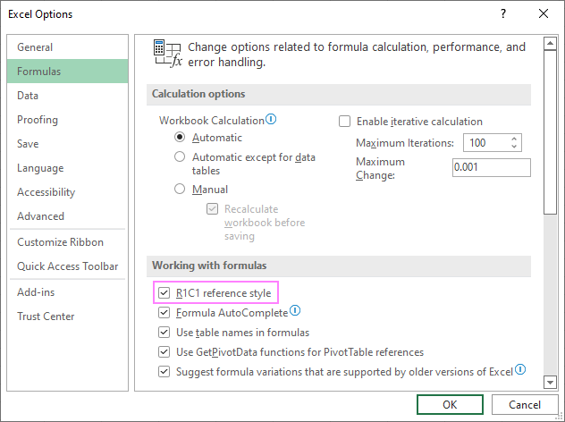
The column labels will immediately change from letters to numbers: 
Please note that selecting this option will not only change column labels — cell addresses will also change from A1 to R1C1 references, where R means «row» and C means «column». For example, R1C1 refers to the cell in row 1 column 1, which corresponds to the A1 reference. R2C3 refers to the cell in row 2 column 3, which corresponds to the C2 reference.
In existing formulas, cell references will update automatically, while in new formulas you will have to use the R1C1 reference style.
Tip. To revert back to A1 style, uncheck the R1C1 reference style check box in Excel Options.
How to number columns in Excel
If you are not used to the R1C1 reference style and want to keep A1 references in your formulas, then you can insert numbers in the first row of our worksheet, so you have both — column letters and numbers. This can be easily done with the help of the Auto Fill feature.
Here are the detailed steps:
- In A1, type number 1.
- In B1, type number 2.
- Select cells A1 and B1.
- Hover the cursor over a small square in the lower right corner of cell B1, which is called the Fill handle. As you do this, the cursor will change to a thick black cross.
- Drag the fill handle to the right up to the column you need.

As a result, you will retain the column labels as letters, and underneath the letters you will have the column numbers.
Tip. To keep the columns numbers in view while scrolling to the below areas of the worksheet, you can freeze top row.
That’s how to return column numbers in Excel. I thank you for reading and look forward to seeing you on our blog next week!
Источник
If your Microsoft Excel application has column numbers instead of letters, then you may be wondering not only how that happened, but how you can fix it.
We get used to certain things remaining consistent in the computer applications that we use regularly, and that’s especially true of Excel.
So if you have Excel column number labels at the tops of your columns instead of letters, then you can follow our steps below to switch them back.
How to Switch Excel Column Number to Letter
- Open your spreadsheet.
- Select the File tab.
- Choose Options.
- Click the Formulas tab.
- Uncheck the R1C1 reference style box.
- Click OK.
Our guide continues below with additional information to answer the question of why are my columns in Excel numbers, including pictures of these steps.
When you refer to a cell in Microsoft Excel spreadsheets, such as with a subtraction formula, you are likely accustomed to doing so by indicating the column, then the row number.
For example, the top-left cell in your spreadsheet would be cell A1. However, you might be using Excel and find that the columns are labeled with numbers instead of letters.
This can be confusing if you were not expecting it, and have not worked with this setup before.
This cell reference system is called R1C1, and is common in some fields and organizations.
However, it is just a setting in Excel 2013, and you can change it if you would prefer to use the column letters with which you are familiar.
Our guide below will show you how to turn on the R1C1 reference style so that you can go back to column letters instead of numbers.
Read our convert to number Excel guide for information on switching text to numbers in Microsoft Excel spreadsheets.
How to Change Excel 2013 Column Labels from Numbers Back to Letters (Guide with Pictures)
The steps in this article assume that you are currently seeing Excel column labels as numbers instead of letters, and that you would like to switch back. Note that this setting is defined for the Excel application, meaning that it will apply to every spreadsheet that you open in the program.
Step 1: Open Excel 2013.
Step 2: Click the File tab at the top-left corner of the window.
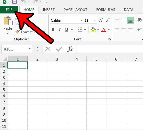
Step 3: Click Options at the bottom of the column on the left side of the window.
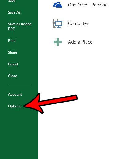
Step 4: Click the Formulas tab at the left side of the Excel Options window.
Step 5: Scroll down to the Working with formulas section of the menu, then uncheck the box to the left of R1C1 reference style. Click the OK button at the bottom of the window to apply your changes.
Now that you know how to switch Excel column numbers to letters you will be able to fix this problem again in the future, should you encounter it.
You should now be returned to your spreadsheet, where the column labels should once again be letters instead of numbers.
Are you having trouble fixing the constant issues that seem to occur whenever you try to print a spreadsheet? Our Excel printing tips can provide you with some helpful pointers and settings that can make printing your data a little less frustrating.
Additional Sources

Matthew Burleigh has been writing tech tutorials since 2008. His writing has appeared on dozens of different websites and been read over 50 million times.
After receiving his Bachelor’s and Master’s degrees in Computer Science he spent several years working in IT management for small businesses. However, he now works full time writing content online and creating websites.
His main writing topics include iPhones, Microsoft Office, Google Apps, Android, and Photoshop, but he has also written about many other tech topics as well.
Read his full bio here.
My column headings are labeled with numbers instead of letters
- On the Excel menu, click Preferences.
- Under Authoring, click General .
- Clear the Use R1C1 reference style check box. The column headings now show A, B, and C, instead of 1, 2, 3, and so on.
Contents
- 1 How do you change Excel to Numbers?
- 2 How do I show column numbers in Excel?
- 3 How do I convert text to values in Excel?
- 4 How do I convert a column of numbers to column names in Excel?
- 5 How do I change the number format in Excel?
- 6 Why does Excel have numbers for columns?
- 7 How do I show columns and row numbers in Excel?
- 8 How do I get columns and row numbers in Excel?
- 9 How do I get row numbers in Excel?
- 10 How do I format numbers in Excel?
- 11 What are the different ways in formatting numbers?
- 12 How do I change the column title in Excel?
- 13 How do I change rows and column names in Excel?
- 14 How do I change Excel columns from numbers to alphabets?
- 15 How do I get rid of column 1 headers in Excel?
- 16 How do I change the row numbers in Excel?
- 17 What is an Xlookup in Excel?
- 18 Why can’t I see row numbers in Excel?
- 19 How do I add a numbered list in Excel?
- 20 How do I automatically number in sheets?
Change numbers with text format to number format in Excel for the…
- Select the cells that have the data you want to reformat.
- Click Number Format > Number. Tip: You can tell a number is formatted as text if it’s left-aligned in a cell.
How do I show column numbers in Excel?
Show column number
- Click File tab > Options.
- In the Excel Options dialog box, select Formulas and check R1C1 reference style.
- Click OK.
How do I convert text to values in Excel?
Use the Format Cells option to convert number to text in Excel
- Select the range with the numeric values you want to format as text.
- Right click on them and pick the Format Cells… option from the menu list. Tip. You can display the Format Cells…
- On the Format Cells window select Text under the Number tab and click OK.
How do I convert a column of numbers to column names in Excel?
To convert a column number to an Excel column letter (e.g. A, B, C, etc.) you can use a formula based on the ADDRESS and SUBSTITUTE functions. With this information, ADDRESS returns the text “A1”.
How do I change the number format in Excel?
You can use the Format Cells dialog to find the other available format codes:
- Press Ctrl+1 ( +1 on the Mac) to bring up the Format Cells dialog.
- Select the format you want from the Number tab.
- Select the Custom option,
- The format code you want is now shown in the Type box.
Why does Excel have numbers for columns?
Cause: The default cell reference style (A1), which refers to columns as letters and refers to rows as numbers, was changed. Solution: Clear the R1C1 reference style selection in Excel preferences. On the Excel menu, click Preferences.The column headings now show A, B, and C, instead of 1, 2, 3, and so on.
How do I show columns and row numbers in Excel?
On the Ribbon, click the Page Layout tab. In the Sheet Options group, under Headings, select the Print check box. , and then under Print, select the Row and column headings check box .
How do I get columns and row numbers in Excel?
It is quite easy to figure out the row number or column number if you know a cell’s address. If the cell address is NK60, it shows the row number is 60; and you can get the column with the formula of =Column(NK60). Of course you can get the row number with formula of =Row(NK60).
How do I get row numbers in Excel?
Use the ROW function to number rows
- In the first cell of the range that you want to number, type =ROW(A1). The ROW function returns the number of the row that you reference. For example, =ROW(A1) returns the number 1.
- Drag the fill handle. across the range that you want to fill.
How do I format numbers in Excel?
Formatting the Numbers in an Excel Text String
- Right-click any cell and select Format Cell.
- On the Number format tab, select the formatting you need.
- Select Custom from the Category list on the left of the Number Format dialog box.
- Copy the syntax found in the Type input box.
What are the different ways in formatting numbers?
How to change number formats. You can select standard number formats (General, Number, Currency, Accounting, Short Date, Long Date, Time, Percentage, Fraction, Scientific, Text) on the home tab of the ribbon using the Number Format menu. Note: As you enter data, Excel will sometimes change number formats automatically.
How do I change the column title in Excel?
Select a column, and then select Transform > Rename. You can also double-click the column header. Enter the new name.
How do I change rows and column names in Excel?
Rename columns and rows in a worksheet
- Click the row or column header you want to rename.
- Edit the column or row name between the last set of quotation marks. In the example above, you would overwrite the column name Gold Collection.
- Press Enter. The header updates.
How do I change Excel columns from numbers to alphabets?
To change the column headings to letters, select the File tab in the toolbar at the top of the screen and then click on Options at the bottom of the menu. When the Excel Options window appears, click on the Formulas option on the left. Then uncheck the option called “R1C1 reference style” and click on the OK button.
How do I get rid of column 1 headers in Excel?
Go to Table Tools > Design on the Ribbon. In the Table Style Options group, select the Header Row check box to hide or display the table headers. If you rename the header rows and then turn off the header row, the original values you input will be retained if you turn the header row back on.
How do I change the row numbers in Excel?
Here are the steps to use Fill Series to number rows in Excel:
- Enter 1 in cell A2.
- Go to the Home tab.
- In the Editing Group, click on the Fill drop-down.
- From the drop-down, select ‘Series..’.
- In the ‘Series’ dialog box, select ‘Columns’ in the ‘Series in’ options.
- Specify the Stop value.
- Click OK.
What is an Xlookup in Excel?
Use the XLOOKUP function to find things in a table or range by row.With XLOOKUP, you can look in one column for a search term, and return a result from the same row in another column, regardless of which side the return column is on.
Why can’t I see row numbers in Excel?
In order to show (or hide) the row and column numbers and letters go to the View ribbon. Set the check mark at “Headings”. That’s it!
How do I add a numbered list in Excel?
Click the Home tab in the Ribbon. Click the Bullets and Numbering option in the new group you created. The new group is on the far right side of the Home tab. In the Bullets and Numbering window, select the type of bulleted or numbered list you want to add to the text box and click OK.
How do I automatically number in sheets?
Use autofill to complete a series
- On your computer, open a spreadsheet in Google Sheets.
- In a column or row, enter text, numbers, or dates in at least two cells next to each other.
- Highlight the cells. You’ll see a small blue box in the lower right corner.
- Drag the blue box any number of cells down or across.
Topics Map > OS and Desktop Applications > Applications > Productivity
Microsoft Excel can be configured to display column labels as numbers instead of letters. This feature is called «R1C1 Reference Style«, and though it can be useful, it can also be confusing if inadvertently enabled.
This document contains instructions for disabling the «R1C1 Reference Style» feature in the following versions of Microsoft Office:
Office 2008/2011 (Mac)
-
Click on the Excel menu at the top of the screen and select Preferences.

-
Click on General.

-
Uncheck R1C1 Reference Style.
-
Click OK at the bottom.


Office 2010/2013 (Win)
-
Click on the File tab at the top of the screen and select Options.

-
Click Formulas.
-
Uncheck R1C1 Reference Style.
-
Click OK at the bottom of the window.


Office 2007 (Win)
-
Click on the Office button in the top left hand corner.
-
Click on Excel Options.

-
Select the Formulas tab on the left.
-
Uncheck R1C1 Reference Style.
-
Click OK at the bottom.


Office 2003 (Win)
-
Click on the Tools menu.
-
Choose Options.
-
Click on the General tab.
-
Uncheck R1C1 Reference Style.
| Keywords: | excel xp 2001 2002 2003 2007 2008 column label number letter r1c1 format display header reference Suggest keywords | Doc ID: | 781 |
|---|---|---|---|
| Owner: | Help Desk KB Team . | Group: | DoIT Help Desk |
| Created: | 2000-11-21 19:00 CDT | Updated: | 2022-08-02 13:18 CDT |
| Sites: | DoIT Help Desk, New Mexico State University, University of Illinois Unified, UW Oshkosh | ||
| Feedback: | 12 2 Comment Suggest a new document |
Friday, March 27th, 2015

What to do when Excel shows Column 1 not Column A
My Excel has been behaving stupidly lately. Instead of Column letters – A, B & C etc, the columns are numbered 1, 2, 3 and so on.
While I haven’t solved the fundamental problem I do have a short term solution. It all has to do with the Excel options. To change the column numbers back to letters chose File (the Office Button in Excel 2007) and choose Options > Formulas and disable the checkbox for R1C1 Reference Style.

On the Mac click Excel > Preferences > General and deselect the Use R1C1 Reference Style checkbox.

This setting kicks Excel back into the correct mode – much more to my taste!
Of course, if you prefer seeing numbers and not letters all you need to do is to click the checkbox and you are good to go!
Labels: change Excel columns to letters, change Excel columns to numbers, column letters, column numbers, columns as numbers, Excel, r1c1, troubleshooting
Labels:office, Windows
- Remove From My Forums
-
Question
-
Using office/excel 2010.
My excel now designates columns with numbers.
Formulas are now written with row and column designations based on change from current cell, not showing the other cell’s address.
I believe a setting must have been changed somehow.
How can I change it back to Letters with columns and formulas that use cell addresses?
Answers
-
On Wed, 7 Dec 2011 19:32:26 +0000, Chuck Peterson wrote:
>
>
>Using office/excel 2010.
>
>My excel now designates columns with numbers.
>
>Formulas are now written with row and column designations based on change from current cell, not showing the other cell’s address.
>
>I believe a setting must have been changed somehow.
>
>How can I change it back to Letters with columns and formulas that use cell addresses?
>
>
Office Buttons/ Excel Options / Formulas / Working with Formulas: DEselect the R1C1 option
Ron
-
Marked as answer by
Thursday, December 8, 2011 3:05 AM
-
Marked as answer by