
Excel Columns to Rows (Table of Contents)
- Columns to Rows in Excel
- How to Convert Columns to Rows in Excel using Transpose?
Columns to Rows in Excel
In Excel, to convert any Columns to Rows, first select the column which you want to switch and copy the selected cells or columns. To proceed further, go to the cell where you want to paste the data. Then from the Paste option, which is under the Home menu tab, select the Transpose option. This will convert the selected Columns into Rows. You can also use the shortcut keys Alt + H + V + T, which will directly take us to the TRANSPOSE function.
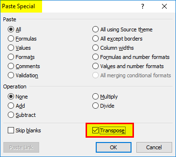
Paste Special Option.
The shortcut key for paste special:
Once you have copied the range of cells that need to be transposed, click on Alt + E + S in a cell where you want to paste special a dialog box popup window with the transpose option.
How to Convert Columns to Rows in Excel using Transpose?
Converting data from column to row in excel is very simple and easy. Let’s understand the working of converting columns to rows by using some examples.
You can download this Convert Columns to Rows Excel Template here – Convert Columns to Rows Excel Template
Example #1
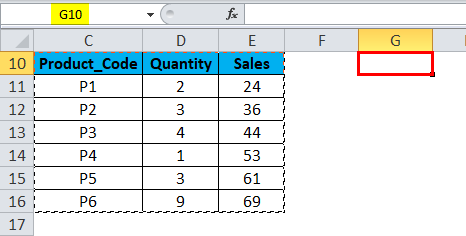
The below-mentioned Pharma sales table contains the medicine product code in column C (C10 to C16), quantity sold in column D (D10 to D16) & total sales value in column E (E10 to E16).
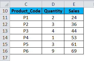
Here we need to convert its orientation from columns to rows with the help of a paste special option in excel.
- Select the whole table range, i.e. all the cells with the dataset in a spreadsheet.
- Copy the selected cells by pressing Ctrl + C.
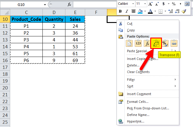
- Select the cell where you want to paste this data set, i.e. G10.
- When you enable right-click on the mouse, the paste option appears. You must then select the 4th option, i.e. Transpose (As mentioned in the below screenshot)
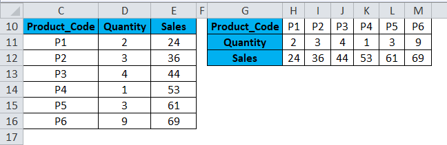
- On selecting the transpose option, your dataset gets copied in that cell range starting from cell G10 to M112.
- Apart from the above procedure, you can also use a shortcut key to convert columns to rows in excel.
- Copy the selected cells by pressing Ctrl + C.
- Select the cell where you need to copy this data set, i.e. G10.
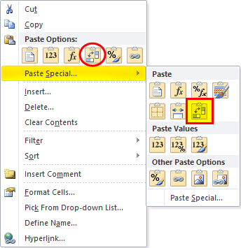
- Click on Alt + E + S, paste special dialog box popup window appears, in that select or click on the box of Transpose option, it will result or convert column data to rows data in excel.
Data that is copied is called source data, and when this source data is copied to other ranges, i.e. pasted data, which is referred to as transposed data.
Note: In the other direction where you are going to copy raw or source data, you have to ensure to select the same number of cells as the original set of cells so that there is no overlapping with the original dataset. In the above-mentioned example, there are 7-row cells that are arranged vertically. So when we copy this dataset to the horizontal direction, it should contain 7 column cells towards the other direction so that the overlapping does not occur with the original dataset.
Example #2
Sometimes, when you have huge number of columns, column data at the end is not visible, and it does not fit to screen. In this scenario, you can change its orientation from the current horizontal range to the vertical range with the help of the paste special option in excel.
- The table contains months and their serial number (From columns C to W).
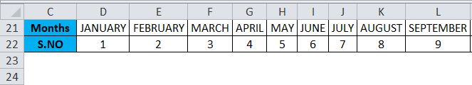
- Select the whole table range, i.e. all the cells with the dataset in a spreadsheet.
- Copy the selected cells by pressing Ctrl + C.
- Select the cell where you need to copy this data set, i.e. C24.
- When you right-click on the mouse, the paste options appear, in that you have to select 4th option, i.e. Transpose (Below mentioned screenshot)
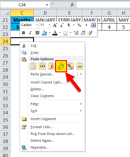
- On selecting the transpose option, your dataset gets copied in that cell range starting from cell C24.
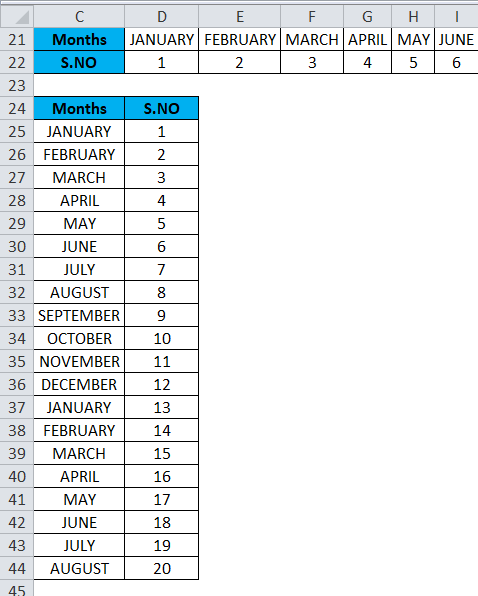
In the transposed data, all the data values are visible and clear as compared to the source data.
Disadvantages of using Paste special option:
- Sometimes copy-paste option creates duplicates.
- If you have used the Paste special option in excel to convert columns to rows, the transposed cells (or arrays) are not linked to each other with source data, and it does not get updated when you try to change data values in source data.
Example #3
Transpose function: It converts columns to rows and rows to columns in excel.
The syntax or formula for the Transpose function is:

- Array: It is a range of cells that you need to convert or change their orientation.
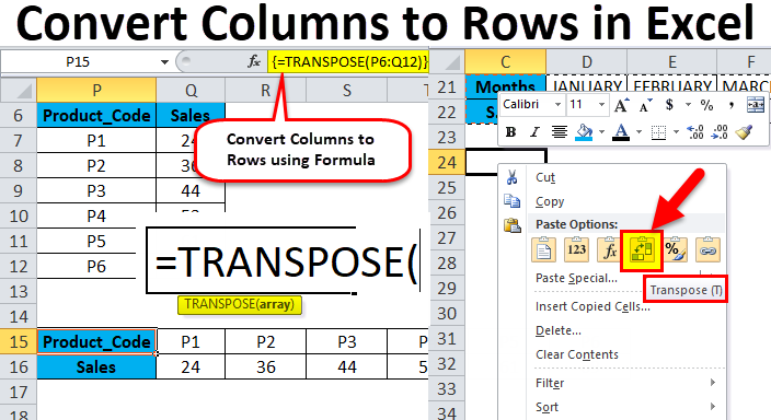
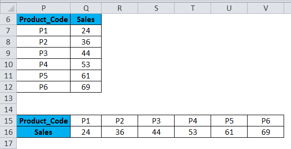
In the below example, the Pharma sales table contains medicine product code in column P (P7 to P12), and sales data in column Q (Q7 to Q12).
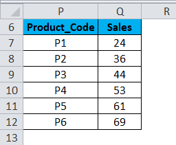
Check out the number of rows & columns in the source data which you want to transpose.
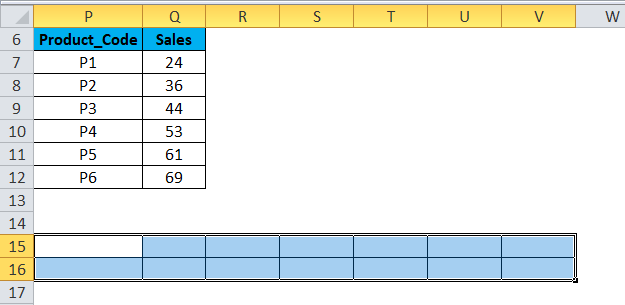
i.e. Initially, count the number of rows and columns in your original source data (7 rows & 2 columns) which is vertically positioned. Now select the same number of blank cells, but in the other direction (Horizontal), i.e. (2 rows & 7 columns)
- Prior to entering the formula, select the empty cells, i.e. from P15 to V16.
- With the empty cells selected, Type the transpose formula in cell P15. i.e. = TRANSPOSE (P6:Q12).
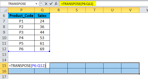
- Since the formula needs to be applied for the whole range, press Ctrl + Shift + Enter to make it an array formula.
Now you can check the dataset; here, columns are converted to rows with datasets.
Advantages of the TRANSPOSE function:
- The main benefit or advantage of using the TRANSPOSE function is that transposed data or the rotated table retains the connection with the source table data, and whenever you change the source data, the transposed data also changes accordingly.
Things to Remember about Convert Columns to Rows in Excel
- Paste special option can also be used for other tasks, i.e. Add, Subtract, Multiply, and Divide between datasets.
- #VALUE error occurs while selecting the cells, i.e. If the number of columns and rows selected in transposed data are not equal to the rows and columns of the source data.
Recommended Articles
This has been a guide to Columns to Rows in Excel. Here we have discussed how to convert columns to rows in excel using transpose along with practical examples and a downloadable excel template. Transpose can help everyone to convert multiple Columns to Rows in excel easily and quickly. You can also go through our other suggested articles –
- COLUMNS Formula in Excel
- Add Rows in Excel Shortcut
- Column Header in Excel
- VBA Columns
In this article, we will learn how to switch the row value into column value and column value into row value through Transpose formula in Excel.
Problem is: -Transposing the values in List1 (cells A2:A5) into a row, and the values in List2 (cells B10:F10) in to a column.
In Excel, we have Transpose formula to update the column data in row and row data in column. Also, we can use Index function along with Row function to convert the row data in column, and we will use a combination of Index function and column function to convert the column data in row.
Let’s take an example and understand how we can transpose the values:-
To transpose the values in Column A (List1) into a Row:

Follow below given steps:-
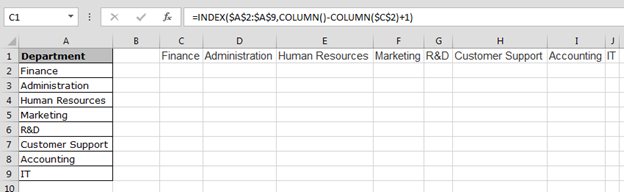
- Enter the formula in cell C1.
- =INDEX($A$2:$A$9,COLUMN()-COLUMN($C$2)+1), and press Enter.
- Copy the formula C1:I1.

We can use Transpose function. Let’s see how we use the Transpose function.
- Select the range C1:I1 and press F2.
- Enter the formula in cell =TRANSPOSE(A2:A5)
- Press Ctrl+Shift+Enter on your keyboard.
How to transpose from a Row into a Column?
We have data in range A1:I1, and we want to update this data in range A2:A9.

- Enter the formula in cell A2.
- =INDEX($B$1:$I$1,ROW()-ROW($K$1)), and press Enter.
- Copy the formula A2:A9.

We can use Transpose function as well. Now, let’s see how we can use the Transpose function.
- Select the range A2:A9 and press F2.
- Enter the formula in cell =TRANSPOSE(B1:I1)
- Press Ctrl+Shift+Enter on your keyboard.

This is the way we can update the row data into column and column data into row through formula in Excel.
Below you can find more example to learn about Transpose:-
How to transpose cells in Microsoft Excel
How to use Transpose function
How to Transpose in Microsoft Excel 2007
How to Copy Vertical and Paste Horizontal in Microsoft Excel
![]()
If you liked our blogs, share it with your friends on Facebook. And also you can follow us on Twitter and Facebook.
We would love to hear from you, do let us know how we can improve, complement or innovate our work and make it better for you. Write us at info@exceltip.com
We all look at data differently. For example, some people create Microsoft Excel spreadsheets with the main fields horizontal. Others prefer data flipped vertically in columns. Sometimes these preferences lead to a scenario where you want to switch data. In this tutorial, I’ll show how to switch rows and columns using the Transpose feature.
The Layout Problem
I was recently given a large Microsoft Excel spreadsheet that contained vendor evaluation information. The information was useful, but I couldn’t use tools like Auto Filter because of the way the data was organized. I would also have issues if I needed to import the original source table into a database. A simple example is shown below.

Instead, I want to have the Company names displayed vertically in Column A and the Data Attributes displayed horizontally in Row 1. This would make it easier for me to do the analysis. For example, I can’t easily filter for California vendors with the original table.
What is Excel’s Transpose Function
In simple terms, the transpose feature changes your columns’ orientation (vertical range) and rows (horizontal range). My original data rows would become columns, and my columns would become rows. So this fixes my layout problem above without me having to retype my original data. And the system would adjust for column labels.
The transpose function is pretty versatile. For example, you can use the feature in Excel formulas or with paste options. However, there are some differences based on which method you use.
Convert Columns to Rows Using Paste Special
The steps outlined below were done using Microsoft Office 365, but recent Microsoft Excel versions will work.
- Open the spreadsheet you need to change. You may also download the example sheet at the end of this tutorial.
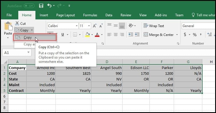
- Click the first cell in your cell range such as A1.
- Shift-click the last cell of the range. Your data set should highlight.
- From the Home tab, select Copy or type Ctrl + c.
- Select the new cell where you would like to copy your transposed data.
- Right-click in that cell and select the Transpose icon from the Paste Options.

✪ As you hover over the Paste options, you can see the data layout change.
You should now see Excel switched the columns and rows. You can resize your columns to suit your needs.
These two data sets are independent. You can delete cells from the top set and it will not impact the transposed set.

When using this method, your original formatting is maintained. For example, if I added a yellow background to my original cells B1:G1, the same background color would be applied. The same is true if I used red text on cell E:5.
Use Transpose Function in a Formula
As I mentioned, Excel has multiple ways for you to switch columns to rows or vice versa. This second way utilizes a formula and array. The result is the same except your original data, and the new transposed data are linked. As a result, you may lose some of your original formatting. For example, colored text and styles came across, but not cell fill colors.
- Open your Excel sheet.
- Click a blank cell where you want your converted data. I’m using A7.
- Type =transpose.
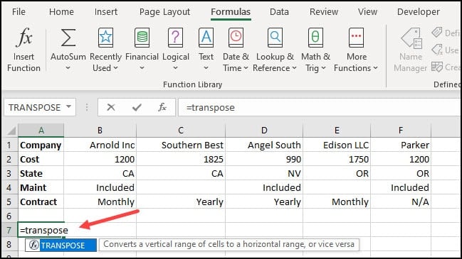
✪ Notice how Excel provides a tooltip showing for Transpose – “Converts a vertical range of cells to a horizontal range and vice versa“.
- Finish the formula by adding a ( and highlighting the cell range we wish to swap.
- Type ) to close the range.
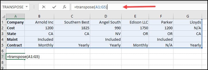
- Press Enter.
✪ If you’re not using Microsoft 365, you’ll probably need to press CTRL + SHIFT + Enter
Differences in Transpose Options
While these two methods produce similar results, there are differences. In the first paste method, whatever action I take on a cell is independent of the transposed version. I could delete the original values, and nothing would happen to the columns I swapped.
In contrast, the Transpose formula version is tethered to the original data. So, for example, if I change the value in B2 from 1200 to 1500, the new value will automatically update in B8. However, the reverse isn’t true. If I change any transposed cells, the original set will not change. Instead, I will get a #SPILL error, and my transposed data will disappear.

Transpose Formula & Blank Cells
Another difference with using the Transpose formula is it will convert blank cells to “0”s.

The fix for this quirk is to use an IF statement to the formula that keeps the blanks cells as blanks.
=TRANSPOSE(IF(A1:G5="","",A1:G5))Alternatively, you could do a search and replace on the zeros.
Now that we’ve shown you how to transpose data in Excel, try playing around with the practice worksheet below. You’ll be swapping your rows and columns in Excel in no time. And while you likely work with multiple rows, you can convert one Excel column to row.
Show Me How Video
Click the image below to see a short video showing how to switch columns and rows without a formula.
![]()
Tutorial Resources
Hand-picked Tutorials
- Beginner’s Guide to XLOOKUP
- How to Use Excel VLOOKUP
- How to Use Excel Auto Filter
- How to Extract Text from a Cell in Excel
- How to Highlight Cells in Excel with Conditional Formatting
The problem is not that we lack data, it’s that we have so much data that it’s hard to find meaning inside of it. You need a way to re-arrange and clean up your data to make it usable. Microsoft Excel is a very user-friendly tool, but you still need to clean up your data before it’s usable for analysis and review.
That’s where Power Query comes into play. Power Query, also called «Get and Transform Data» lives inside of Excel and automates the data cleanup process.
One of the most popular data cleanup steps is to take data that’s spread across columns and convert it into rows of data. Take your Excel skills to the next level by «unpivoting» your data using Microsoft Power Query. In this tutorial, you’ll learn how to use Power Query to convert columns into rows in Excel.
Why Convert Columns to Rows?
Before we get started, you might be wondering why it’s so helpful to take data that’s structured in many columns and convert it into rows.
The answer that is a bit technical. Basically, it’s preferable if each row of data is like a record, a single data point. Columnar data is mixed up with multiple attributes spread across columns.
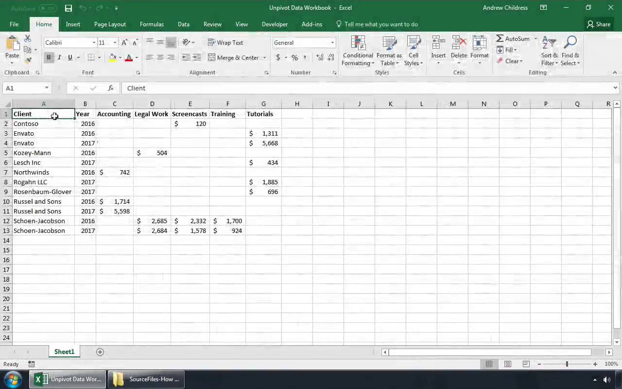
In the example below, you can see what data looks like when you convert it from columns to rows in Excel. On the left side is a set of client records, with different project types in columns. On the right side, I’ve unpivoted the data and converted it to a row format.


Also, if you’re a Pivot Table user, it’s very important that your data is in rows instead of columns when you use it to create a Pivot Table. Data in columns simply doesn’t feed Pivot Tables correctly.
In short: converting data from columns to rows makes it easier to work with. Power Query makes this an easy, two click operation. Let’s learn how:
How To Quickly Convert Columns To Rows In Excel (Watch & Learn)
If you’ve never used Power Query before, I’d highly recommend checking out this quick, two minute screencast below to watch me work with it. You’ll learn how to take your columnar data and convert it into rows (records) in Excel to make it easier to work with.
Let’s also walk through a written version of these instructions to learn more about Power Query and «unpivoting» data in Excel.
Meet Microsoft Power Query for Excel
Power Query, which is formally called «Get and Transform Data» in Excel 2016, is a tool with two main functions:
- You can use it to get data, such as pointing it to other Excel files, databases, and even web pages to pull data down and into a spreadsheet.
- It can help you transform data, which means rearranging it on the fly, adding more columns, or merging other sets of data with it.


Power Query is a deep and powerful tool that lives inside of Excel. Instead of manually rearranging data and repeating the process, Power Query lets you build a set of steps that you can apply to your data repeatedly.
Installing Power Query
Power Query is built into Excel 2016, but you can install it for earlier versions of Excel as an add-in. Unfortunately, Power Query is only available for Excel on Windows.
To install Power Query for Excel on Windows, (only needed for Excel 2013 for Excel 2010, as this feature is built into Excel 2016) jump over to Microsoft’s website to download and install the Power Query add-in.
Send Data to Power Query
Power Query is used inside of Excel, but it opens up in a new window that sits on top of Excel.
To unpivot data in Excel, you’ll first need to convert your Excel data into a table if it’s not already in that format. You can hand off a data table to Power Query to work with your data.
If you’d like to follow along with me in this tutorial, I’ve made the sample data available in this free Excel file.
Convert to Table
To convert data into a table, click anywhere inside the table and then find the Format as Table option that’s on Excel’s ribbon. You can click on any of the style thumbnails to convert your flat cells into a data table.


Handoff to Power Query
Once your data is in a table format, go to the Data tab on Excel’s ribbon, and click on the From Table button to send the table data to Power Query to transform your data.


This sends the data into a new window that opens inside of, but on top of Microsoft Excel. It’s an entirely new window with a ton of features.
Unpivot Data
At this point, you should see something similar to the screenshot below. This is the window that holds the tools you need to unpivot.
To unpivot the data in Excel, highlight all of the columns that you want to unpivot. Basically, Power Query will transform each of these columns into rows of their own. For the sample data here, I’ve highlighted each of the columns for the project types:


Once you’ve clicked on Unpivot Columns, Excel will transform your columnar data into rows. Each row is a record of its own, ready to throw into a Pivot Table or work with in your datasheet.


This feature feels like magic. Now, let’s send the data back over to Microsoft Excel to work with.
Close & Load
The Power Query window has many features that you can dive into with other tutorials, but for now, we’re finished with unpivoting our data. Let’s go ahead and click on the Close & Load button to send data back to Excel.


Close and Load sends data back to Excel, and puts it in a spreadsheet. You’ll also see a queries window on the right side that shows the query that we just built to unpivot data.
Refresh the Query
So, what if your original data changes? If you have more rows added to the original data, you don’t have to repeat this entire process in order to unpivot those rows.
Instead of recreating the query from scratch, you need to use the Refresh Data option. In the screenshot below, I’ll add an entirely new row for a brand new client to my original data source:


Now, let’s return to the tab where our unpivoted data is loaded. When we click inside of the table, you’ll see the Workbook Queries menu open next to your data. Press the Refresh button (right side of the menu) to refresh the query.
This action looks back at the original table and re-runs the query steps. Because we’ve added new rows to our original data table, Power Query adds these new rows to the query and runs them through the unpivot transformation.


This is one of my favorite features about Power Query. We added data to the original source, but one click has refreshed it and unpivoted the new data as well.
Recap and Keep Learning More About Using Microsoft Excel
In this tutorial, you learned how easy it is to convert columns to rows in Microsoft Excel. Power Query is a flexible and robust tool to grab and rearrange your data on the fly. Continue learning more Microsoft Excel techniques in these Envato Tuts+ tutorials:
How do you use Power Query or other tools to unpivot your data? If you have a favorite tip to share, make sure to check in with a comment below.
Did you find this post useful?

I believe that life is too short to do just one thing. In college, I studied Accounting and Finance but continue to scratch my creative itch with my work for Envato Tuts+ and other clients. By day, I enjoy my career in corporate finance, using data and analysis to make decisions.
I cover a variety of topics for Tuts+, including photo editing software like Adobe Lightroom, PowerPoint, Keynote, and more. What I enjoy most is teaching people to use software to solve everyday problems, excel in their career, and complete work efficiently. Feel free to reach out to me on my website.
This question is stale but I just needed it, so I’ll answer.
I found the solution by Chris Chua on Quora, please upvote him there if this is helpful: https://www.quora.com/How-do-I-convert-multiple-column-data-into-a-column-with-multiple-rows-in-excel
I’ll also copy-paste it here in case of a broken link:
Apologies. I can’t really see the writings clearly, but I’m assuming that you want to unpivot the column headers as part of the data set.
Here I am suggesting a solution using Microsoft Excel’s Power Query feature. If you have Excel 2016, the feature is found under Data | Get & Transform ribbon command. Otherwise if you have Excel 2013 or the Professional Plus version of 2010, you can download the Power Query add-in from here.
Step 1: Select all the data, press Ctrl+T to create a table, and under Create Table, make sure that My table has headers is selected.
Sample data create table dialog
Step 2: In Excel 2016, go to Data | Get & Transform | From Table. For Power Query add-in for Excel 2013 and 2010, look for something in the Power Query tab ribbon that says From Table.
Ribbon location for «From Table»
Step 3: The Power Query interface will open up. Click on the header of No. Column, hold Ctrl and click on the header of the Name Column. With both columns now selected, right click on the headers and select Unpivot Other Columns.
Right Click, Unpivot Other Columns screencap
Step 4: Notice that the data is now unpivoted (which is what you wanted). Double click on the Attribute and Value headers to rename them.
Step 5: Click Home | Close & Load.
Close & Load screencap
Step 6: Excel will load the new cleaned up table onto a new sheet. Ta-da you’re done!
Screencap of pivoted table, which is the desired output.
To update any new data in the future:
Supposed you now have new data in your original table.
Updated sample data table screencap with a new column, row and value inserted.
Go to the new cleaned up table, right click and select Refresh.
Screencap of right-clicking inside the pivoted output table, clicking Refresh.
The new data will be updated immediately.
Get and Transform
The “Get and Transform” tools have been widely available since Excel 2016. Prior to 2016, the tools were available via a free download as part of the Power Query toolset.
The Problem
Our dataset contains sales for a year grouped by month (blue), and each row represents an App/Type grouping (yellow).

We want to transpose the monthly data and combine it with the App/Type data. Our result should have
- 12 rows for “WenCaL/Sales” (Jan…Dec)
- 12 rows for “WenCaL/Volume” (Jan…Dec)
- 12 rows for “WenCaL/Returns” (Jan…Dec), etc.
Problem with Blanks
One of the issues with traditional transpose strategies is wherever an empty cell exists, no row will be created for that App/Type combination.
To solve this issue, we will need to “zero fill” all the empty cells in the range of numbers.
Step 1 – Pull the Data into Power Query
The Power Query suite of tools (located in the “Get and Transform” group on the Data tab) will allow us to quickly and easily correct this data.
Click anywhere in the data (anywhere in A3:N12) and select Data (tab) -> Get & Transform Data (group) -> From Table/Range.

Provided there are no completely blank rows or columns in the data, the Create Table dialog box’s selection range should be correct. If not, make the necessary adjustments. Also, make sure the “My table has headers” option is selected then click OK.

The data will be sent to the Power Query Editor for further processing.
The Power Query Editor is an entire suite of tools used to fix virtually any data irregularity or data transformation issue.

The first thing we will do is to select the Name field from the Query Settings -> Properties panel on the right and change the name to something more meaningful, like “TableFinal”.

Step 2 – Fix the Data
Our first task will be to replace all the empty value cells with zeroes. Empty cells will be skipped in the next step when we transpose the table. Since we don’t want chronological gaps in our data, we need to occupy the empty cells with a value.

NOTE: In Power Query, an empty cell is labeled as a “null” cell. This is just a fancy way to say “empty” in Power Query.
We have 12 columns of monthly data to replace nulls with zeroes.
Click the header of the “Jan” column, scroll to the right, hold CTRL then click the header of the “Dec” column.
With the 12 month columns highlighted, select Home (tab) -> Transform (group) -> Replace Values.

In the Replace Values dialog box, type “null” (no quotation marks) in the Value To Find field, and a “0” (no quotation marks) in the Replace With field and click OK.

All the “null” cells have been replaced with zeroes.

Step 3 – Transposing the Months
The next step is to transpose the month columns and create associated entries for each corresponding App/Type combination.
We could select the month columns like we did earlier and then transpose them but imagine if instead of 12 month columns there were 1,000 product columns.
A faster method would be to select the two columns that we will be reproducing, the App and Type columns, and then instruct Power Query to fix all the OTHER columns, leaving our selected columns out of the process.
Select the App and Type columns, then select Transform (tab)-> Any Column (group) -> click the small arrow next to Unpivot Columns -> Unpivot Other Columns.

The data has been transposed.

Step 4 – Loading the Results into Excel
To load the results into Excel, select Home (tab) -> Close (group)-> Close & Load.

We have our transposed list in Excel as an official Excel Table.

We can now create Pivot Tables, Charts, filter, and sort to our heart’s delight.
3 Ways to Transpose
Change Horizontal Data to Vertical
Unstack Data from One Column to Many Columns
Practice Workbook
Feel free to Download the Workbook HERE.
![]()
Published on: September 19, 2019
Last modified: February 28, 2023


Leila Gharani
I’m a 5x Microsoft MVP with over 15 years of experience implementing and professionals on Management Information Systems of different sizes and nature.
My background is Masters in Economics, Economist, Consultant, Oracle HFM Accounting Systems Expert, SAP BW Project Manager. My passion is teaching, experimenting and sharing. I am also addicted to learning and enjoy taking online courses on a variety of topics.
In Excel one can easily convert data columns to rows or multiple data rows to columns which is technically named transpose.
What is Transpose?
In Excel switching or rotating columns to rows or rows to columns is called Transposing the data.
And this actually shifts the dimensions of data and along with it definitely the address of different data bits will also change. Therefore, if you are into transposing your data, do it with caution as if you shift the data the dependent cells might miscalculate the figures.
Love reading about Excel? Subscribe my youtube channel dedicated to Excel.
[vc_btn title=”Subscribe” style=”custom” custom_background=”#ff0000″ custom_text=”#ffffff” size=”lg” align=”right” i_icon_fontawesome=”fa fa-youtube-play” add_icon=”true” link=”url:https%3A%2F%2Fgoo.gl%2Fx16inH||target:%20_blank|”]
Many already know how to do this. But for those who don’t this one minute Excel tutorial is for them. By the way, yes! you can use pivot tables to shift rows as columns. To learn how to make pivot tables read this readers’ favourite tutorial. And most probably you will figure out the way how rows are shifted as columns using pivot tables.
We have several ways to switch or rotate Excel data columns to rows or vice versa to accomplish this task. Following are the transpose methods we are discussing today in which few involve converting columns to rows using Excel formulas:
- Use Paste Special
- Use TRANSPOSE function
- Use INDIRECT function
- Use INDEX function
- Use Paste Special + Common Sense
Method 1: Convert columns to rows using Paste Special
Copying and Pasting is one great thing happened to PC. With Paste Special it really went miles ahead. In Excel you can copy a data and then using paste special functionality you can twist, rotate, manipulate, process and do other things with the data very easily including Transpose i.e. flipping columns to rows or rows to columns. To do this following steps will help:
Step 1: Select the data that you want to transpose and copy it using the copy button or with Ctrl+C shortcut.
Step 2: Go to the cell where you want the data to paste. And go to Home tab > clip board group > click the drop down button just under paste button > select:
- under paste sub-group click transpose button that comes with this icon; OR
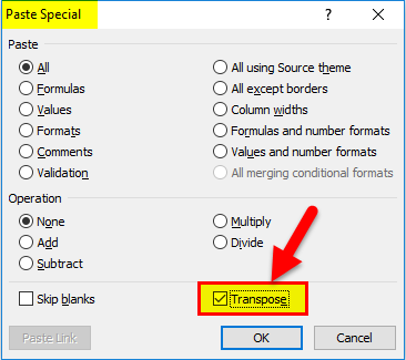
- Select paste special. This will open the paste special dialogue from which check the transpose checkbox and click OK button
Your data will be transposed instantly. Told ya! it is easy!
Method 2: TRANSPOSE Function to switch columns to rows or vice versa
Yes there is a function that can do the somersault called TRANSPOSE. The use of this function is a little tricky and requires knowing more than pressing TAB so follow the steps closely.
IMPORTANT: Determine the rows and columns of your data. For example you have 2 columns and 7 rows. Once you transpose the data it will be 2 rows and 7 columns.
Step 1: Determine the rows and columns of data. In our case it is 7 rows and 2 columns
Step 2: Select a vacant region in the worksheet which is 2 rows deep and 7 columns wide.
Step 3: Press F2 key to enter edit mode while the region still selected.
Step 4: Write TRANSPOSE function following the equal sign and enter the data range that you want to transpose
Step 5: Hit CTRL+SHIFT+ENTER. Yes! Not just Enter key but Ctrl+Shift+Enter as this is an array formula
TANGO! Your data is transposed!
Benefit of TRANSPOSE Function
The best thing with using TRANSPOSE function is that if you change the values in the source range then transposed range will also change accordingly. So basically it is a live-transposed-range of the source-range.
But as this is an array function this is very much dependent on the source and if you try to change anything this tends to break. Therefore, even if it is good for many reasons, it is hard go by in many situations. So follow along to learn some more easier to go tricks to get the data transposed in Excel.
Method 3: TRANSPOSE Using INDIRECT function
INDIRECT function was introduced in one of my favourite article some time back in which we learned how to build a reference to worksheet based on cell value. I must confess that I used to think INDIRECT has very little use but this little function can prove tremendous help.
Today we will look at another use of INDIRECT function i.e. to transpose the data. However, if you use this function the treatment for column to row shift is a little different from row to column shift. So I will explain both one by one.
Transpose – Column to Row using INDIRECT
Suppose our data is based on 2 columns A and B and 7 rows from 1 to 7.
The data of column A has address like A1, A2, A3,…. A7. In this A is constant whereas due to additional rows we have increasing numbers from 1 to 7. If you understand up to this, you will understand what we are about to learn.
Lets say you want to put the transposed data starting at cell C10. I will put this formula in cell C10 and press Enter key:
=INDIRECT(“A”&COLUMN()-2)
And this formula in C11 and press Enter:
=INDIRECT(“B”&COLUMN()-2)
Now select these two cells and drag the fill handle across to column I. So there you have the data transposed. But lets understand what formula is actually doing.
Understanding INDIRECT approach to TRANSPOSE
As told earlier Indirect formula helps in converting text strings to cell references. COLUMN function actually gives us the number of column in which the formula is entered. For example if you put =COLUMN in any cell of column A it will give the value of 1 as it is first column. Similarly if you put the COLUMN function in any cell of column I, it will return 9 as it is 9th column.
So with the column function we were able to incremental numbers as we drag the formula across columns. But as we inserted the formula in third column and the not first column so it would have returned 3 in which case the first address to be fetched would have been A3. But we want the values from first cell of column A therefore we had to insert “-2”. This way we got 1, 2, 3 and not 3, 4, 5
So the formula: =INDIRECT(“A”&COLUMN()-2)
In the above formula “A” is provided as text string which is joined (concatenated) using “&” with the values generated through COLUMN function. And thus successfully built the cell references.
Now if you change the values in source range the transposed range will also change. But it is much more flexible as it won’t break if you change one item in transposed range manually.
Transpose – Rows to Columns using INDIRECT
Using the same technique learnt above, we can transpose the data from rows to columns. But in this case you will use ROWS() function instead of COLUMNS to work correctly.
As you are converting rows to columns therefore you will be going down the rows and thus you require number increments as rows are jumped. So simply adjust the formula as per your needs and use ROW instead of COLUMN and it will do the rest for you.
No you can’t simply replace the COLUMN function with ROW function as mentioned above to convert the rows back to columns. Instead you will have to use the combination of INDIRECT, ADDRESS and ROW function.
In my case to transpose first row to column I used the formula: =INDIRECT(ADDRESS(10,ROW()-11))
Whereas to convert the second row to column I used this formula: =INDIRECT(ADDRESS(11,ROW()-11))

Method 4: TRANSPOSE using INDEX functions
Using the technique learnt to transpose columns to rows above. You can use INDEX function if building reference is difficult for you and you still have your head spinning.
INDEX function is one great addition to Excel functions and formulas repository. Lets have a look at the syntax of INDEX very briefly so that we understand how can we use it to transpose the data.
INDEX(array, row_num, [column_num])
array: the range, in our case it is the range we want to transpose
row_num: the row number. In this function we have mention row number to help it fetch the value
[column_num]: this is the optional argument. If not mentioned the column number doesn’t change and it will be the same in which function is applied. But today we need this option badly!
Transposing Rows to Columns using INDEX function
Suppose our data is arranged from cell A1 to G2. Two rows and seven columns in other words. So if we transpose the data we will have 2 columns and 7 rows.
To transpose the data arranged in a row to column go to the cell from where you want the data to start. I selected cell C6 and D6 and put theses formula:
Cell C6: =INDEX($A$1:$G$2,1,ROW()-5)
Cell D6: =INDEX($A$1:$G$2,2,ROW()-5)
Select both cells and drag the fill handle down to next six rows i.e. row 12. And you will get the data transposed from rows to columns.
Understanding the formula
Lets take some time to understand the mechanics of this formula. The formula we applied in cell C6 is as follows:
=INDEX($A$1:$G$2,1,ROW()-5)
array: [$A$1:$G$2] – this is the range that we want to transpose. The reference is made absolute so that as we drag the formula this array stays static and does not change.
row_num: [1] – this represent the first row of the data and we mentioned it so that INDEX function recognize that we want it to fetch the values only from row 1 of selected array i.e. $A$1:$G$2.
column_num: [ROW()-5] – Our data A, B, C, … G is in one row but across 7 columns. That means the address of:
- value A is first row-first column
- value B is first row-second column
- value C is first row-third column; and so on…
So as we drag the formula down, we want the formula to get the values from 1st, 2nd, 3rd, 4th, 5th, 6th and 7th column. To do this we have to tell the column number. Now one way is to mention column number manually every time we put the INDEX function in next cell so that it fetches the right value.
But to automate the process of feeding column numbers to the function, I used ROW() function as the argument of column number (column_num). And as I drag the fill handle down, the ROW function will churn out row numbers inside the formula.
ROW function gives the row number. Now as I have put the INDEX function cell C6 the ROW function will tell that ROW number is 6. But we want it to be 1 as I want to fetch the values from the first column of the selected array. That is the reason we have “-5” following ROW() inside the formula. So it reduces the numbers generated by ROW function by 5 and this it will give 1, 2, 3, … 7.
Transposing Columns to Rows using INDEX function
Once you understand how INDEX function has fetched the values in above situation. Its easy to understand how to tackle the data which is arranged in columnar form and we want it to shift in rows.
For this we will make two changes:
for row_num: now we will use COLUMN() function generate numbers so that as we drag the formula towards right the row number will get updated because we are jumping across columns and thus COLUMN function will fetch the column number. Adjust the value generated by column number by adding or subtracting constants so that you get the desired result.
for column_num: mention 1 or 2 depending on the column within the selected array from which you want the values fetched.
Example
For example my data is based in 2 columns 7 rows and is housed in column C and D starting at Row 6.
I want the data transposed in rows 13 and 14 in column F. Therefore I put these formula:
cell F13:
=INDEX($C$6:$D$12,COLUMN()-5,1)
cell F14:
=INDEX($C$6:$D$12,COLUMN()-5,2)
Select both cells and drag to the right until column L
Method 5: Paste Special + Common Sense = Paste Ultimate!
We saw TRANSPOSE function went ahead of Paste Special as it was not only able push columns as rows (transpose) but were also live as transposed range was able to update as source change. We fixed some of the TRANSPOSE nuisances through INDIRECT approach. But writing formula and then dragging the range takes time.
But can we get TRANSPOSE like result using paste special? The answer is yes!
Paste Link
To get the live feed of source range we can use Paste Special’s inhouse capability called Paste link. Paste link pastes the cell references and not the values in cell and if source data changes, the linked cell will also change.
However, for unknown reasons, if you try to transpose and paste link at the same time Excel does not allow that i.e. you can either transpose or paste link. In other words, if you click Paste Link button with transpose option checked, the moment you select transpose option the paste link button gets disabled.
To get around this misery we took help of our Agent-X named common sense. Follow along!
Step 1: Copy the range and go to any vacant space in the same worksheet.
Step 2: Hit Alt+Ctrl+V to invoke paste special dialogue box and hit the button paste link. This will paste NOT the cell values but the cell references of the range you copied.
Step 3: Select the range you just pasted and hit Ctrl+H. This will bring up the REPLACE dialogue.
Step 4: In ‘Find what’ field mention equal sign i.e. “=” (without quotes) and in replace with field mention “HS=” and hit Replace ALL button. This will actually convert the formula into text as you have just replaced the equal sign with HS=
Step 5: Copy the range again and now go to the place where you want to put the transposed range. Hit Alt+Ctrl+V to bring the paste special dialogue box. Select the Transpose option and click OK. This will effectively transpose the data.
Step 6: To revert the formulas back in place so that you get the correct values in place from the source range. Hit Ctrl+H again. This time in Find what field put HS= and in replace with mention =. Hit Replace ALL button.
Now you have the live-transposed-range of the source WITHOUT using TRANSPOSE function or similar alternatives. How cheeky was that! 😉
So how do you do the transpose? If you have new ideas or any better versions of the ideas discussed do let me know in the comment section
If you have a worksheet with data in columns that you need to rotate to rearrange it in rows, use the Transpose feature. With it, you can quickly switch data from columns to rows, or vice versa.
For example, if your data looks like this, with Sales Regions in the column headings and and Quarters along the left side:
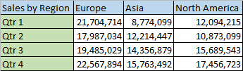
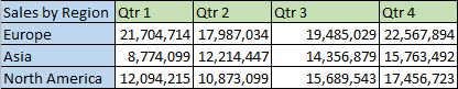
The Transpose feature will rearrange the table such that the Quarters are showing in the column headings and the Sales Regions can be seen on the left, like this:
Note: If your data is in an Excel table, the Transpose feature won’t be available. You can convert the table to a range first, or you can use the TRANSPOSE function to rotate the rows and columns.
Here’s how to do it:
-
Select the range of data you want to rearrange, including any row or column labels, and press Ctrl+C.
Note: Ensure that you copy the data to do this, since using the Cut command or Ctrl+X won’t work.
-
Choose a new location in the worksheet where you want to paste the transposed table, ensuring that there is plenty of room to paste your data. The new table that you paste there will entirely overwrite any data / formatting that’s already there.
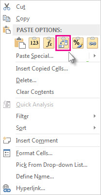
Right-click over the top-left cell of where you want to paste the transposed table, then choose Transpose
 .
.
-
After rotating the data successfully, you can delete the original table and the data in the new table will remain intact.
 .
.
Tips for transposing your data
-
If your data includes formulas, Excel automatically updates them to match the new placement. Verify these formulas use absolute references—if they don’t, you can switch between relative, absolute, and mixed references before you rotate the data.
-
If you want to rotate your data frequently to view it from different angles, consider creating a PivotTable so that you can quickly pivot your data by dragging fields from the Rows area to the Columns area (or vice versa) in the PivotTable Field List.
You can paste data as transposed data within your workbook. Transpose reorients the content of copied cells when pasting. Data in rows is pasted into columns and vice versa.
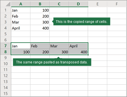
Here’s how you can transpose cell content:
-
Copy the cell range.
-
Select the empty cells where you want to paste the transposed data.
-
On the Home tab, click the Paste icon, and select Paste Transpose.

30 Aug How to Track Excel Template Submission Versions
Howdee! A big part of some analyst’s job is usually collecting data via templates and aggregating that data into reports for leaders to review. This presents a problem. Many times, the way users want to enter data, is not favorable for aggregating reports or inserting data into a database. This can lead to complex formulas and lots potential issues. Let’s look at a revenue forecast document for example. Typically, you’ll send a document where each column represents a month of the fiscal year. However, month really should be a single field from a data perspective. Turning Excel columns to rows of data is a common requirement when aggregating data. Fortunately, there exists an effortless way of accomplishing this, and it has the added benefit of allowing you to version your data submissions!
Prep the Data
As with most things in Excel, getting the data ready is most of the battle. In this case, you need to closely examine what column’s you’re wanting moved to row data and what other data needs to be included to make sense of it. I’ve made this example data below to demo this:

In this simple example, we have a monthly forecast, the revenue streams the forecast represents, and who submitted it. The reason to decide beforehand, is that we need to consolidate all the columns we want in our final data set into one “key” column. This may sound strange, but it will make sense shortly. Beyond combining the columns, we need to delimit them so we can separate them for later use. I typically concatenate them with the pipe (shift + backslash key to get “|”) delimiter. However, if any of your columns contain pipes, you’ll need to reconsider which key to delimit with.
Next, we need to make sure that there are no blank cells in the columns we want to move to row data. If the cell is blank, that result will be missing from our final data. If that won’t affect you, then you may not need to worry about this, but I’ve found it to have adverse effects depending on what I am doing with that final data. Lastly, we need to make sure all the columns we want to perform the columns to rows action on are grouped together and that our “key” column is inserted directly beside it. The result is a column of data that looks like this:

A side note here, since some of you might be questioning the “CONCAT” formula vs. “CONCATENATE”. That came with a recent Microsoft update for Office 365 users a few months ago. The only difference is that CONCAT accepts range inputs where CONCATENATE is limited to one cell per input. This is helpful when you need to concatenate several fields together to make a unique ID for a row.
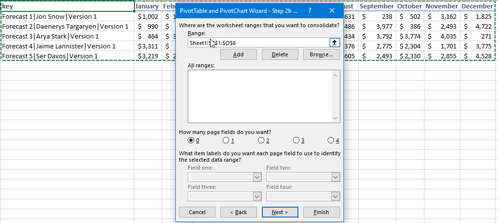
Moving on, the next step is to use a little-known shortcut to access the old Office menu. I don’t think that many people are aware that, pressing “Alt + D” allows you to access some of the older functionality of Excel. In this case, the full shortcut is “Atl + D + P”. Some of you may remember this old user interface for creating pivot tables through the pivot table wizard. There are a lot more options that affect how the data is stored inside of the cube. For us we want to first select the “Multiple consolidation ranges” radio button, and keep the “PivotTable” radio button selected in the second option and click next. In the second window, select the “I will create the page fields” option and click next. Finally, click the up arrow next to the Range box, and select your range. It should only include the “key” column, and the columns we want to move to rows.
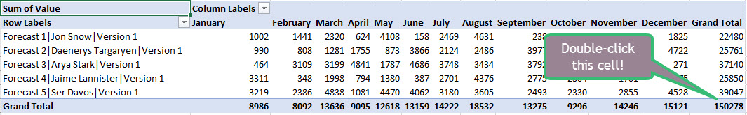
Once you select finish, you’ll be directed to a new worksheet where you’re pivot table will be populated. It will look just like the data you selected to be pivoted except it will have totals for columns and rows. This means everything worked great! Also, if you did have blank cells in the data you select to be pivoted, you’ll most likely end up with a PivotTable that reflects counts instead of sums. It’s not a big deal if that data isn’t important to you but, if it is, you’ll need to back up a few steps and get rid of those blank cells. A find and replace typically works for me.
Next, double click on the cell of the pivot table where the grand total for rows intersects the grand total for columns. See picture below for example:
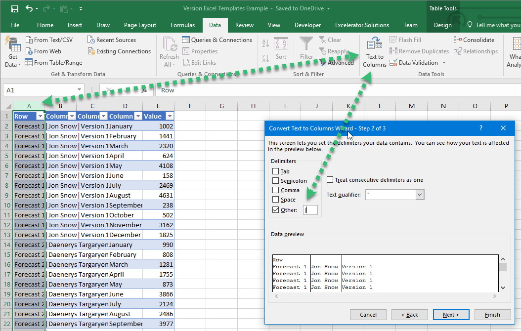
The result of this will be a data table with three columns. The first will be the concatenated “key” column. The second will be the “columns to rows” columns. Finally, the third will be the values from those columns. The last step is to expand our concatenated column back out so we have all the data we want back in one spot. Immediately to the right of the first column, I will insert two columns (one for the extra field and I concatenated and one for the version). Then use the “Text To Columns” functionality to un-concatenate your string as pictured below. You will get an error telling you there is text already here but don’t worry, that’s just because of the table column headers. Finally, rename your columns and you have a brand new data set where all of your values are in one column and you know what submission version this came from!
Summary
Discovering this method literally changed everything about the way I handled reporting. I could easily compare submissions side by side and see what changed from the previous submission. Before, I had to use incredibly complex formulas linked across multiple files to do this. Now I just keep adding to a data table, pivot the results, and I can compare any submission I’ve previously stored using this approach. Hopefully you find this excel columns to rows example as helpful as I have over the years.
As usual, I’ve saved this file in the “Example Files” section of my site. If you’re a subscriber, you can download it for free. It just takes a minute to sign up. It’s free and I won’t spam you with tons of unwanted emails. If you have questions on anything in this article, drop them in the comments below!
Cheers,
R