
In a Data Model, each column has an associated data type that specifies the type of data the column can hold: whole numbers, decimal numbers, text, monetary data, dates and times, and so on. Data type also determines what kinds of operations you can do on the column, and how much memory it takes to store the values in the column.
If you’re using the Power Pivot add-in, you can change a column’s data type. You might need to do this if a date column was imported as a string, but you need it to be something else. For more information, see Set the data type of a column in Power Pivot.
In this article
-
Summary of data types
-
Table Data Type
-
-
Implicit and explicit data type conversion in DAX formulas
-
Table of Implicit Data Conversions
-
Addition (+)
-
Subtraction (-)
-
Multiplication (*)
-
Division (/)
-
Comparison operators
-
-
-
Handling blanks, empty strings, and zero values
Summary of data types
The following table lists data types supported in a Data Model. When you import data or use a value in a formula, even if the original data source contains a different data type, the data is converted to one of these data types. Values that result from formulas also use these data types.
|
Data type in Excel |
Data type in DAX |
Description |
|---|---|---|
|
Whole Number |
A 64 bit (eight-bytes) integer value 1, 2 |
Numbers that have no decimal places. Integers can be positive or negative numbers, but must be whole numbers between -9,223,372,036,854,775,808 (-2^63) and 9,223,372,036,854,775,807 (2^63-1). |
|
Decimal Number |
A 64 bit (eight-bytes) real number 1, 2 |
Real numbers are numbers that can have decimal places. Real numbers cover a wide range of values: Negative values from -1.79E +308 through -2.23E -308 Zero Positive values from 2.23E -308 through 1.79E + 308 However, the number of significant digits is limited to 15 decimal digits. |
|
TRUE/FALSE |
Boolean |
Either a True or False value. |
|
Text |
String |
A Unicode character data string. Can be strings, numbers or dates represented in a text format. Maximum string length is 268,435,456 Unicode characters (256 mega characters) or 536,870,912 bytes. |
|
Date |
Date/time |
Dates and times in an accepted date-time representation. Valid dates are all dates after January 1, 1900. |
|
Currency |
Currency |
Currency data type allows values between -922,337,203,685,477.5808 to 922,337,203,685,477.5807 with four decimal digits of fixed precision. |
|
N/A |
Blank |
A blank is a data type in DAX that represents and replaces SQL nulls. You can create a blank by using the BLANK function, and test for blanks by using the logical function, ISBLANK. |
1 DAX formulas do not support data types smaller than those listed in the table.
2 If you try to import data that has very large numeric values, import might fail with the following error:
In-memory database error: The ‘<column name>’ column of the ‘<table name>’ table contains a value, ‘1.7976931348623157e+308’, which is not supported. The operation has been cancelled.
This error occurs because Power Pivot uses that value to represent nulls. The values in the following list are synonyms for the null value:
|
Value |
|
|---|---|
|
9223372036854775807 |
|
|
-9223372036854775808 |
|
|
1.7976931348623158e+308 |
|
|
2.2250738585072014e-308 |
Remove the value from your data and try importing again.
Table Data Type
DAX uses a table data type in many functions, such as aggregations and time intelligence calculations. Some functions require a reference to a table; other functions return a table that can then be used as input to other functions. In some functions that require a table as input, you can specify an expression that evaluates to a table; for some functions, a reference to a base table is required. For information about the requirements of specific functions, see DAX Function Reference.
Implicit and explicit data type conversion in DAX formulas
Each DAX function has specific requirements as to the types of data that are used as inputs and outputs. For example, some functions require integers for some arguments and dates for others; other functions require text or tables.
If the data in the column you specify as an argument is incompatible with the data type required by the function, DAX in many cases will return an error. However, wherever possible DAX will attempt to implicitly convert the data to the required data type. For example:
-
You can type a date as a string, and DAX will parse the string and attempt to cast it as one of the Windows date and time formats.
-
You can add TRUE + 1 and get the result 2, because TRUE is implicitly converted to the number 1 and the operation 1+1 is performed.
-
If you add values in two columns, and one value happens to be represented as text («12») and the other as a number (12), DAX implicitly converts the string to a number and then does the addition for a numeric result. The following expression returns 44: = «22» + 22
-
If you attempt to concatenate two numbers, Excel will present them as strings and then concatenate. The following expression returns «1234»: = 12 & 34
The following table summarizes the implicit data type conversions that are performed in formulas. Excel performs implicit conversions whenever possible, as required by the specified operation.
Table of Implicit Data Conversions
The type of conversion that is performed is determined by the operator, which casts the values it requires before performing the requested operation. These tables list the operators, and indicate the conversion that is performed on each data type in the column when it is paired with the data type in the intersecting row.
Note: Text data types are not included in these tables. When a number is represented as in a text format, in some cases Power Pivot will attempt to determine the number type and represent it as a number.
Addition (+)
|
Operator (+) |
INTEGER |
CURRENCY |
REAL |
Date/time |
|---|---|---|---|---|
|
INTEGER |
INTEGER |
CURRENCY |
REAL |
Date/time |
|
CURRENCY |
CURRENCY |
CURRENCY |
REAL |
Date/time |
|
REAL |
REAL |
REAL |
REAL |
Date/time |
|
Date/time |
Date/time |
Date/time |
Date/time |
Date/time |
For example, if a real number is used in an addition operation in combination with currency data, both values are converted to REAL, and the result is returned as REAL.
Subtraction (-)
In the following table the row header is the minuend (left side) and the column header is the subtrahend (right side).
|
Operator (-) |
INTEGER |
CURRENCY |
REAL |
Date/time |
|---|---|---|---|---|
|
INTEGER |
INTEGER |
CURRENCY |
REAL |
REAL |
|
CURRENCY |
CURRENCY |
CURRENCY |
REAL |
REAL |
|
REAL |
REAL |
REAL |
REAL |
REAL |
|
Date/time |
Date/time |
Date/time |
Date/time |
Date/time |
For example, if a date is used in a subtraction operation with any other data type, both values are converted to dates, and the return value is also a date.
Note: Data models also supports the unary operator, — (negative), but this operator does not change the data type of the operand.
Multiplication (*)
|
Operator (*) |
INTEGER |
CURRENCY |
REAL |
Date/time |
|---|---|---|---|---|
|
INTEGER |
INTEGER |
CURRENCY |
REAL |
INTEGER |
|
CURRENCY |
CURRENCY |
REAL |
CURRENCY |
CURRENCY |
|
REAL |
REAL |
CURRENCY |
REAL |
REAL |
For example, if an integer is combined with a real number in a multiplication operation, both numbers are converted to real numbers, and the return value is also REAL.
Division (/)
In the following table the row header is the numerator and the column header is the denominator.
|
Operator (/) (Row/Column) |
INTEGER |
CURRENCY |
REAL |
Date/time |
|---|---|---|---|---|
|
INTEGER |
REAL |
CURRENCY |
REAL |
REAL |
|
CURRENCY |
CURRENCY |
REAL |
CURRENCY |
REAL |
|
REAL |
REAL |
REAL |
REAL |
REAL |
|
Date/time |
REAL |
REAL |
REAL |
REAL |
For example, if an integer is combined with a currency value in a division operation, both values are converted to real numbers, and the result is also a real number.
Comparison operators
In comparison expressions Boolean values are considered greater than string values and string values are considered greater than numeric or date/time values; numbers and date/time values are considered to have the same rank. No implicit conversions are performed for Boolean or string values; BLANK or a blank value is converted to 0/»»/false depending on the data type of the other compared value.
The following DAX expressions illustrate this behavior:
=IF(FALSE()>»true»,»Expression is true», «Expression is false»), returns «Expression is true»
=IF(«12″>12,»Expression is true», «Expression is false»), returns «Expression is true».
=IF(«12″=12,»Expression is true», «Expression is false»), returns «Expression is false»
Conversions are performed implicitly for numeric or date/time types as described in the following table:
|
Comparison Operator |
INTEGER |
CURRENCY |
REAL |
Date/time |
|---|---|---|---|---|
|
INTEGER |
INTEGER |
CURRENCY |
REAL |
REAL |
|
CURRENCY |
CURRENCY |
CURRENCY |
REAL |
REAL |
|
REAL |
REAL |
REAL |
REAL |
REAL |
|
Date/time |
REAL |
REAL |
REAL |
Date/time |
Top of Page
Handling blanks, empty strings, and zero values
In DAX, a null, blank value, empty cell, or a missing value are all represented by the same new value type, a BLANK. You can also generate blanks by using the BLANK function, or test for blanks by using the ISBLANK function.
How blanks are handled in operations, such as addition or concatenation, depends on the individual function. The following table summarizes the differences between DAX and Microsoft Excel formulas, in the way that blanks are handled.
|
Expression |
DAX |
Excel |
|---|---|---|
|
BLANK + BLANK |
BLANK |
0 (zero) |
|
BLANK +5 |
5 |
5 |
|
BLANK * 5 |
BLANK |
0 (zero) |
|
5/BLANK |
Infinity |
Error |
|
0/BLANK |
NaN |
Error |
|
BLANK/BLANK |
BLANK |
Error |
|
FALSE OR BLANK |
FALSE |
FALSE |
|
FALSE AND BLANK |
FALSE |
FALSE |
|
TRUE OR BLANK |
TRUE |
TRUE |
|
TRUE AND BLANK |
FALSE |
TRUE |
|
BLANK OR BLANK |
BLANK |
Error |
|
BLANK AND BLANK |
BLANK |
Error |
For details on how a particular function or operator handles blanks, see the individual topics for each DAX function, in the section, DAX Function Reference.
Top of Page
readxl::read_excel() will guess column types, by
default, or you can provide them explicitly via the
col_types argument. The col_types argument is
more flexible than you might think; you can mix actual types in with
"skip" and "guess" and a single type will be
recycled to the necessary length.
Here are different ways this might look:
Type guessing
If you use other packages in the tidyverse, you are probably
familiar with readr, which
reads data from flat files. Like readxl, readr also provides column type
guessing, but readr and readxl are very different under the hood.
- readr guesses column type based on the data.
- readxl guesses column type based on Excel cell types.
Each cell in an Excel spreadsheet has its own type. For all intents
and purposes, they are:
empty < boolean < numeric < text
with the wrinkle that datetimes are a very special flavor of numeric.
A cell of any particular type can always be represented as one of any
higher type and, possibly, as one of lower type. When guessing,
read_excel() keeps a running “maximum” on the cell types it
has seen in any given column. Once it has visited guess_max
rows or run out of data, this is the guessed type for that column. There
is a strong current towards “text”, the column type of last resort.
Here’s an example of column guessing with deaths.xlsx
which ships with readxl.
read_excel(readxl_example("deaths.xlsx"), range = cell_rows(5:15))
#> # A tibble: 10 × 6
#> Name Profe…¹ Age Has k…² `Date of birth` `Date of death`
#> <chr> <chr> <dbl> <lgl> <dttm> <dttm>
#> 1 David Bow… musici… 69 TRUE 1947-01-08 00:00:00 2016-01-10 00:00:00
#> 2 Carrie Fi… actor 60 TRUE 1956-10-21 00:00:00 2016-12-27 00:00:00
#> 3 Chuck Ber… musici… 90 TRUE 1926-10-18 00:00:00 2017-03-18 00:00:00
#> 4 Bill Paxt… actor 61 TRUE 1955-05-17 00:00:00 2017-02-25 00:00:00
#> # … with 6 more rows, and abbreviated variable names ¹Profession,
#> # ²`Has kids`Excel types, R types, col_types
Here’s how the Excel cell/column types are translated into R types
and how to force the type explicitly in col_types:
| How it is in Excel | How it will be in R | How to request in col_types
|
|---|---|---|
| anything | non-existent | "skip" |
| empty |
logical, but all NA
|
you cannot request this |
| boolean | logical |
"logical" |
| numeric | numeric |
"numeric" |
| datetime | POSIXct |
"date" |
| text | character |
"text" |
| anything | list |
"list" |
Some explanation about the weird cases in the first two rows:
- If a column falls in your data rectangle, but you do not want an
associated variable in the output, specify the column type
"skip". Internally, these cells may be visited in order to
learn their location, but they are not loaded and their data is never
read. - You cannot request that a column be included but filled with
NAs. Such a column can arise naturally, if all the cells
are empty, or you can skip a column (see previous point).
Example of skipping and guessing:
read_excel(
  readxl_example("deaths.xlsx"),
  range = cell_rows(5:15),
  col_types = c("guess", "skip", "guess", "skip", "skip", "skip")
)
#> # A tibble: 10 × 2
#>   Name            Age
#>   <chr>         <dbl>
#> 1 David Bowie      69
#> 2 Carrie Fisher    60
#> 3 Chuck Berry      90
#> 4 Bill Paxton      61
#> # … with 6 more rows
More about the "list" column type in the last row:
- This will create a list-column in the output, each component of
which is a length one atomic vector. The type of these vectors is
determined using the logic described above. This can be useful if data
of truly disparate type is arranged in a column.
We demonstrate the "list" column type using the
clippy.xlsx sheet that ship with Excel. Its second column
holds information about Clippy that would be really hard to store with
just one type.
(clippy <-
   read_excel(readxl_example("clippy.xlsx"), col_types = c("text", "list")))
#> # A tibble: 4 × 2
#>   name                 value
#>   <chr>                <list>
#> 1 Name                 <chr [1]>
#> 2 Species              <chr [1]>
#> 3 Approx date of death <dttm [1]>
#> 4 Weight in grams      <dbl [1]>
tibble::deframe(clippy)
#> $Name
#> [1] "Clippy"
#>
#> $Species
#> [1] "paperclip"
#>
#> $`Approx date of death`
#> [1] "2007-01-01 UTC"
#>
#> $`Weight in grams`
#> [1] 0.9
sapply(clippy$value, class)
#> [[1]]
#> [1] "character"
#>
#> [[2]]
#> [1] "character"
#>
#> [[3]]
#> [1] "POSIXct" "POSIXt"
#>
#> [[4]]
#> [1] "numeric"
Final note: all datetimes are imported as having the UTC timezone,
because, mercifully, Excel has no notion of timezones.
When column guessing goes wrong
It’s pretty common to expect a column to import as, say, numeric or
datetime. And to then be sad when it imports as character instead. Two
main causes:
Contamination by embedded missing or bad data of incompatible
type. Example: missing data entered as ?? in a
numeric column.
- Fix: use the
naargument ofread_excel()
to describe all possible forms for missing data. This should prevent
such cells from influencing type guessing and cause them to import as
NAof the appropriate type.
Contamination of the data rectangle by leading or trailing
non-data rows. Example: the sheet contains a few lines of
explanatory prose before the data table begins.
- Fix: specify the target rectangle. Use
skipand
n_maxto provide a minimum number of rows to skip and a
maximum number of data rows to read, respectively. Or use the more
powerfulrangeargument to describe the cell rectangle in
various ways. See the examples forread_excel()help or
vignette("sheet-geometry")for more detail.
The deaths.xlsx sheet demonstrates this perfectly.
Here’s how it imports if we don’t specify range as we did
above:
deaths <- read_excel(readxl_example("deaths.xlsx"))
#> New names:
#> • `` -> `...2`
#> • `` -> `...3`
#> • `` -> `...4`
#> • `` -> `...5`
#> • `` -> `...6`
print(deaths, n = Inf)
#> # A tibble: 18 × 6
#>    `Lots of people`             ...2               ...3  ...4  ...5  ...6
#>    <chr>                        <chr>              <chr> <chr> <chr> <chr>
#>  1 simply cannot resist writing NA                 NA    NA    NA    some…
#>  2 at                           the                top   NA    of    thei…
#>  3 or                           merging            NA    NA    NA    cells
#>  4 Name                         Profession         Age   Has … Date… Date…
#>  5 David Bowie                  musician           69    TRUE  17175 42379
#>  6 Carrie Fisher                actor              60    TRUE  20749 42731
#>  7 Chuck Berry                  musician           90    TRUE  9788  42812
#>  8 Bill Paxton                  actor              61    TRUE  20226 42791
#>  9 Prince                       musician           57    TRUE  21343 42481
#> 10 Alan Rickman                 actor              69    FALSE 16854 42383
#> 11 Florence Henderson           actor              82    TRUE  12464 42698
#> 12 Harper Lee                   author             89    FALSE 9615  42419
#> 13 Zsa Zsa Gábor                actor              99    TRUE  6247  42722
#> 14 George Michael               musician           53    FALSE 23187 42729
#> 15 Some                         NA                 NA    NA    NA    NA
#> 16 NA                           also like to writ… NA    NA    NA    NA
#> 17 NA                           NA                 at t… bott… NA    NA
#> 18 NA                           NA                 NA    NA    NA    too!
Non-data rows above and below the main data rectangle are causing all
the columns to import as character.
If your column typing problem can’t be solved by specifying
na or the data rectangle, request the "list"
column type and handle missing data and coercion after import.
Peek at column names
Sometimes you aren’t completely sure of column count or order, and
yet you need to provide some information via
col_types. For example, you might know that the column
named “foofy” should be text, but you’re not sure where it appears. Or
maybe you want to ensure that lots of empty cells at the top of “foofy”
don’t cause it to be guessed as logical.
Here’s an efficient trick to get the column names, so you can
programmatically build the col_types vector you need for
your main reading of the Excel file. Let’s imagine I want to force the
columns whose names include “Petal” to be text, but leave everything
else to be guessed.
(nms <- names(read_excel(readxl_example("datasets.xlsx"), n_max = 0)))
#> [1] "Sepal.Length" "Sepal.Width"  "Petal.Length" "Petal.Width"
#> [5] "Species"
(ct <- ifelse(grepl("^Petal", nms), "text", "guess"))
#> [1] "guess" "guess" "text"  "text"  "guess"
read_excel(readxl_example("datasets.xlsx"), col_types = ct)
#> # A tibble: 150 × 5
#>   Sepal.Length Sepal.Width Petal.Length Petal.Width Species
#>          <dbl>       <dbl> <chr>        <chr>       <chr>
#> 1          5.1         3.5 1.4          0.2         setosa
#> 2          4.9         3   1.4          0.2         setosa
#> 3          4.7         3.2 1.3          0.2         setosa
#> 4          4.6         3.1 1.5          0.2         setosa
#> # … with 146 more rows
Square pegs in round holes
You can force a column to have a specific type via
col_types. So what happens to cells of another type? They
will either be coerced to the requested type or to an NA of
appropriate type.
For each column type, below we present a screen shot of a sheet from
the built-in example type-me.xlsx. We force the first
column to have a specific type and the second column explains what is in
the first. You’ll see how mismatches between cell type and column type
are resolved.
Logical column
A numeric cell is coerced to FALSE if it is zero and
TRUE otherwise. A date cell becomes NA. Just
like in R, the strings “T”, “TRUE”, “True”, and “true” are regarded as
TRUE and “F”, “FALSE”, “False”, “false” as
FALSE. Other strings import as NA.
df <- read_excel(readxl_example("type-me.xlsx"), sheet = "logical_coercion",
                 col_types = c("logical", "text"))
#> Warning: Expecting logical in A5 / R5C1: got a date
#> Warning: Expecting logical in A8 / R8C1: got 'cabbage'
print(df, n = Inf)
#> # A tibble: 10 × 2
#>    `maybe boolean?` description
#>    <lgl>            <chr>
#>  1 NA               "empty"
#>  2 FALSE            "0 (numeric)"
#>  3 TRUE             "1 (numeric)"
#>  4 NA               "datetime"
#>  5 TRUE             "boolean true"
#>  6 FALSE            "boolean false"
#>  7 NA               ""cabbage""
#>  8 TRUE             "the string "true""
#>  9 FALSE            "the letter "F""
#> 10 FALSE            ""False" preceded by single quote"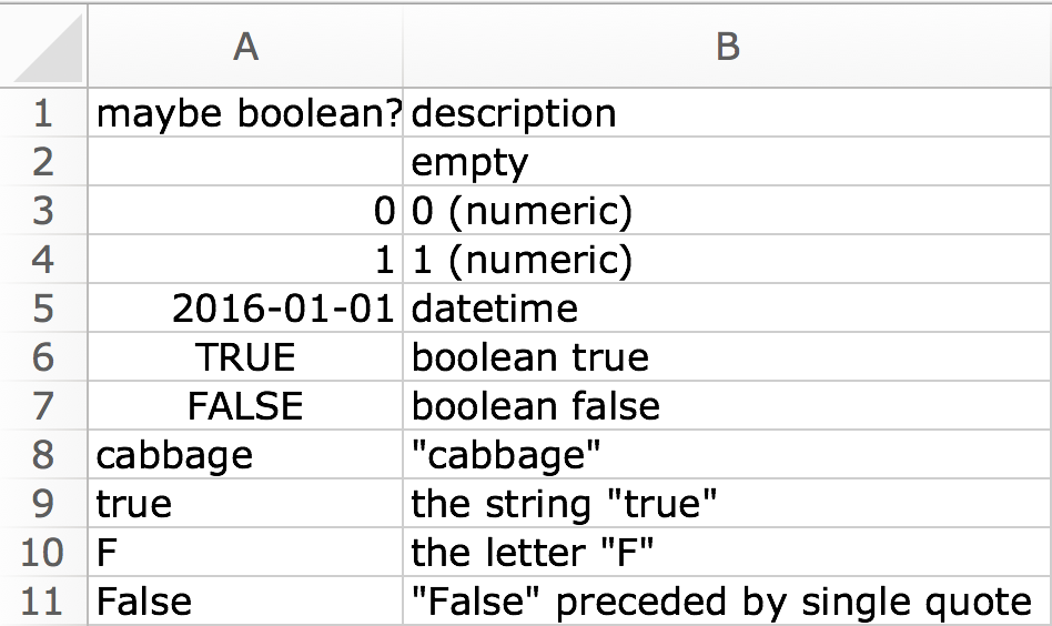
Numeric column
A boolean cell is coerced to zero if FALSE and one if
TRUE. A datetime comes in as the underlying serial date,
which is the number of days, possibly fractional, since the date
origin. For text, numeric conversion is attempted, to handle the
“number as text” phenomenon. If unsuccessful, text cells import as
NA.
df <- read_excel(readxl_example("type-me.xlsx"), sheet = "numeric_coercion",
                 col_types = c("numeric", "text"))
#> Warning: Coercing boolean to numeric in A3 / R3C1
#> Warning: Coercing boolean to numeric in A4 / R4C1
#> Warning: Expecting numeric in A5 / R5C1: got a date
#> Warning: Coercing text to numeric in A6 / R6C1: '123456'
#> Warning: Expecting numeric in A8 / R8C1: got 'cabbage'
print(df, n = Inf)
#> # A tibble: 7 × 2
#>   `maybe numeric?` explanation
#>              <dbl> <chr>
#> 1               NA "empty"
#> 2                1 "boolean true"
#> 3                0 "boolean false"
#> 4            40534 "datetime"
#> 5           123456 "the string "123456""
#> 6           123456 "the number 123456"
#> 7               NA ""cabbage""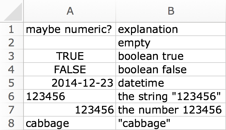
Date column
A numeric cell is interpreted as a serial date (I’m questioning
whether this is wise, but https://github.com/tidyverse/readxl/issues/266).
Boolean or text cells become NA.
df <- read_excel(readxl_example("type-me.xlsx"), sheet = "date_coercion",
                 col_types = c("date", "text"))
#> Warning: Expecting date in A5 / R5C1: got boolean
#> Warning: Expecting date in A6 / R6C1: got 'cabbage'
#> Warning: Coercing numeric to date in A7 / R7C1
#> Warning: Coercing numeric to date in A8 / R8C1
print(df, n = Inf)
#> # A tibble: 7 × 2
#>   `maybe a datetime?` explanation
#>   <dttm>              <chr>
#> 1 NA                  "empty"
#> 2 2016-05-23 00:00:00 "date only format"
#> 3 2016-04-28 11:30:00 "date and time format"
#> 4 NA                  "boolean true"
#> 5 NA                  ""cabbage""
#> 6 1904-01-05 07:12:00 "4.3 (numeric)"
#> 7 2012-01-02 00:00:00 "another numeric"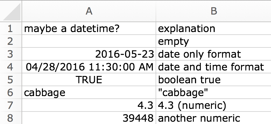
Text or character column
A boolean cell becomes either "TRUE" or
"FALSE". A numeric cell is converted to character, much
like as.character() in R. A date cell is handled like
numeric, using the underlying serial value.
df <- read_excel(readxl_example("type-me.xlsx"), sheet = "text_coercion",
                 col_types = c("text", "text"))
print(df, n = Inf)
#> # A tibble: 6 × 2
#>   text     explanation
#>   <chr>    <chr>
#> 1 NA       "empty"
#> 2 cabbage  ""cabbage""
#> 3 TRUE     "boolean true"
#> 4 1.3      "numeric"
#> 5 41175    "datetime"
#> 6 36436153 "another numeric"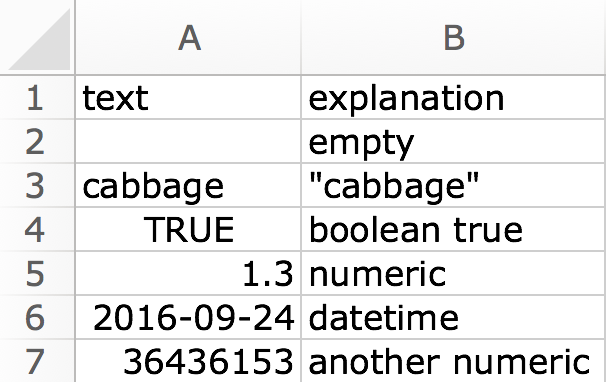
Since the start of Excel, one cell could only contain one piece of data.
With Excel’s new rich data type feature, this is no longer the case. We now have multiple data fields inside one cell!
When you think of data types you might be thinking about text, numbers, dates or Boolean values, but these new data types are quite different. They are really connections to an online data source that provides more information about the data.
At present there are two data types available in Excel; Stocks and Geography.
For example, with the new stock data type our cell might display the name of a company, but will also contain information like the current share price, trading volume, market capitalization, employee head count, and year of incorporation for that company.
The connections to the additional data are live, which is especially relevant for the stock data. Since data like the share price is constantly changing, you can always get the latest data by refreshing the connection.
Caution: The stock data is provided by a third party. Data is delayed, and the delay depends on which stock exchange the data is from. Information about the level of delay for each stock exchange can be found here.
The data connection for the geography data type is also live and can be refreshed, but these values should change very infrequently.
Video Tutorial
Converting Text To Rich Data Types
Whichever data type you want to use, converting cells into a data type is the same process. As you might expect, the new data types have been placed in the Data tab of the Excel ribbon in a section called Data Types.
At present the two available data types fit nicely into the space. But you can click on the lower right area to expand this space, which seems to suggest more data types are on their way!
You will need to select the range of cells with your text data and go to the Data tab and click on either the Stock or Geography data type. This will convert the plain text into a rich data type.
Warning: You can’t convert cells containing formula to data types.
You can easily tell when a cell contains a data type as there will be a small icon on the left inside the cell. The Federal Hall icon indicates a Stock data type and the map icon indicates a Geography data type.
Right Click Data Type Menu
The right click menu has a contextual option which is only available when the right click is performed on a cell or range containing data types. This is where you’ll find most commands related to data types.
Automatic Data Type Conversion
If you want to add to your list of data type cells, all you need to do is type in the cell directly below a data type and Excel will automatically convert it to the same data type as above.
Correcting Missing Data Types
Excel will try and convert your text with the best match, but it might not always find a suitable match or there might be some ambiguity. When this happens, a question mark icon will appear in the cell. You can click on this icon to help Excel find the best match.
Click on the question mark icon and this will open the Data Selector window pane. You can use the search bar to try and locate the desired result and then click on the Select button to accept one of the options presented.
Changing Data Types
In case Excel made the wrong choice, you can also change a data type. You right click on the data and choose Data Type then Change from the menu. This will also open the Data Selector window pane.
Currency & Cryptocurrency Data
With the stock data type, you can get more than just stocks from a company name. The stock data type can also be used for currency and cryptocurrency conversions.
Currency Exchange Rate Pairs
You can convert pairs of currencies into data types to get exchange rates.
Cryptocurrency Exchange Rate Pairs
You can convert cryptocurrency/currency pairs into data types too. Exchange rates between cryptocurrencies are currently not supported.
Country, State, Province, County & City Data
The geography data type supports most types of geographies. Countries, states, provinces, counties and cities will all work.
The fields available for each type of geography will vary. For example, a country, state, province, or county might have a capital city field, but this field will not be available for a city.
Data Cards
There is a pretty cool way to view the data contained inside a cell that’s been. When you click on the icon for any data type a Data Card will appear.
This is also accessible through the rick click menu. Right click then choose Data Type from the menu then choose Data Card.
Data cards will show all the available data for that cell and may also include a picture related to the data such as a company logo or a country’s flag.
Each piece of data displayed in the card also comes with an Extract to grid button that becomes visible when you hover the mouse cursor over that area. This will extract the data into the next blank cell to the right of the data type.
In the lower right corner of the card, there’s a flag icon. This allows you to report any bad data that might be displayed in the card back to Microsoft.
Extracting Data
The data cards are nice for viewing the data inside a cell, but how can you use this data? There are Extract to grid buttons for each piece of data inside the data cards, but these will only extract data for one cell. What if you want to extract data from many cells?
When you select a range of cells containing data types, an Extract to grid icon will appear at the top right of the selected range. When you click on this, Excel will show a list of all the available data that can be extracted. Unfortunately, you’ll only be able to select one piece of data at a time.
A handy feature with extracting data, is that Excel takes care of the number formatting. Whether you’re extracting a percent, number, currency, date or time, Excel will apply the relevant formatting.
Dot Formulas & FIELDVALUE Function
Extract is probably not the best word to use for the Extract to grid button. If you check the contents of the extracted data, you’ll see it’s a formula reference to the data type cell.
Dot Formula Notation
In fact, you don’t need to use the extract to grid button to create these formulas. You can write them just like any other Excel formula.
= B3.PopulationThe above formula will return the population of Canada.
= B3.Population / B3.AreaThe above formula will give us a density calculation and return 3.7 people per square kilometer.
Thankfully, Excel’s formula IntelliSense will show you all the available fields when you create a cell reference to a data type cell followed by a period. This makes writing data type formulas easy!
Note: When the field name contains spaces, the field reference needs to be encased with square braces.
Formulas only support one dot.
= B3.CapitalThe above formula will return the capital of Canada, which is geographical data.
= B3.Capital.PopulationBut the above formula won’t return the population of the capital city of Canada. To get this information, you would need to extract the capital, then copy and paste the result as a value, then convert that value to a data type, then extract the population.
FIELDVALUE Function
The FIELDVALUE function was introduced with data types and can be used to get the exact same results from a data type cell.
= FIELDVALUE(Value, Field)This new function has two arguments:
- Value is a reference to a data type.
- Field is the name of a field in the data type.
Warning: The FIELDVALUE function does not have IntelliSense for the available fields in a data type.
= FIELDVALUE(B3, "Population")The previous example to return the population of Canada can be written as above using the FIELDVALUE function.
= FIELDVALUE(B3, "Population") / FIELDVALUE(B3, "Area")The previous example to return the population density can be written as above using the FIELDVALUE function.
New FIELD Error Type
A new #FIELD! error has been added to Excel for the dot formulas and FIELDVALUE function. This error can be returned for several reasons.
- The field does not exist for the data type.
- The value referenced in the formula is not a data type.
- The data does not exist in the online service for the combination of value and field.
In the above example, Ireland is returning a #FIELD! error for the abbreviation because this data is missing online.
Refreshing Data
How do you refresh data? Using the Refresh and Refresh All commands found in the Data tab will refresh any data types you have in your spreadsheet.
This means you can use the keyboard shortcuts Alt + F5 (refresh) and Ctrl + Alt + F5 (refresh all) to refresh data types.
Using the Refresh command will refresh all cells in the workbook that are the same data type as your active cell.
The Refresh All command will refresh all cells of any data type.
Warning: Refresh All will also refresh all other connections in the workbook such as pivot tables and power queries.
There is also a refresh method that is proprietary to data types. If you select a cell with a data type, you can right click and choose Data Type from the menu then choose Refresh. This will refresh all cells in the workbook that are the same data type as the selected cell and won’t refresh any other connections like pivot tables or power query.
Unlinking Data
If you no longer want your data connected, you can unlink the data by converting it back to regular text. The only way to do this is to right click on the selected range of data then choose Data Type from the menu and select Change to Text.
Warning: Linking and unlinking data might change your data.
When you convert text to a data type and then convert it back to text, you might not get your original text back exactly as it was. It’s best to create a copy of any text data before converting to a data type so you always have the original text.
Using Tables With Data Types
You don’t need to use Excel tables with data types, but there is a nice bonus feature with tables when extracting data. Excel will create the column headings for you.
Note: You can create an Excel table from the Insert tab with the Table command or using the keyboard shortcut Ctrl + T.
Learn more about Excel tables: Everything You Need to Know About Excel Tables
The Extract to grid button will appear anytime the active cell is inside a table containing data types. The active cell does not need to be on a cell containing a data type.
When there are two or more columns with data type inside a table, the Extract to grid button will be based on the right most column. Unfortunately, this means you can’t extract from any other columns.
Using Sort & Filter With Data Types
Sorting and filtering data types has a nice feature that allows you to sort and filter based on any field even if it hasn’t been extracted.
Note: Turn on the sort and filter toggles for any table or list by using the Ctrl + Shift + L keyboard shortcut.
When you click on the sort and filter toggle of a column of data types, you will be able to select a field from a drop down at the top of the menu. This will change the field which sorting and filtering is based on.
For example, we could select the Year incorporated field and sort our list of companies from oldest to newest, or filter out any company incorporated after the year 2000.
Finding Data Types In A Workbook
Data types are visually distinct because of the icons in cell, so distinguishing between a regular cell and a data type cell is easy. But what if you want to locate all the data type cells in a large workbook? Visual inspection might not be practical.
Since data types are not supported by earlier versions of Excel, the easiest way to locate them in a workbook is with Excel’s check compatibility feature.
Note: Check compatibility can be found in the File tab ➜ Info ➜ Check for Issues ➜ Check Compatibility.
The compatibility checker will list out all the features in the workbook that are not backwards compatible with prior version of Excel. To find any data types, you can look for the words “This workbook contains data types…” in the summary. Each summary will also have a Find hyperlink that will take you to the location and select those cells.
Note: Selecting only Excel 2016 from the Select versions to show button will reduce the results in the compatibility checker and make finding the data types easier.
Conclusions
With rich Data Types you can now get more from your data without leaving Excel to use your favourite search engine.
You can quickly and easily get current financial data, currency rates, cryptocurrency values and geographical data with a couple clicks.
This is a very powerful feature in Excel you need to start using, and with the hint of more data types to come, will become even more useful.
About the Author
John is a Microsoft MVP and qualified actuary with over 15 years of experience. He has worked in a variety of industries, including insurance, ad tech, and most recently Power Platform consulting. He is a keen problem solver and has a passion for using technology to make businesses more efficient.
- Remove From My Forums
-
Question
-
Dear M experts,
I have an Excel table with two columns «Name» and «Type» with the column names and for every column a type (type text, Int64.Type etc.). Now I want a list of names and types for the
Table.TransformColumnTypes-feature. This is what I have tried:
ExcelSource = Excel.CurrentWorkbook(){[Name=»ColumnTypes»]}[Content],
TypeList = Table.ToRows(ExcelSource),
ChangedType = Table.TransformColumnTypes(Source,TypeList)I get the error «Expression.Error: Cannot convert the value «»type text»» to type «Type» «.
Can anyone help?
Answers
-
Hi,
It’s not clear why you’re wanting to do this. Is it to override the types that Power Query automatically sets with the #Changed Type» step?
You could add a step to evaluate the types in text to produce actual type values, but you would get only primitive types after evaluation, e.g. «Int64.Type» will be evaluated as type number.
TransformedTypes = List.Transform(TypeList, each {_{0}} & {Expression.Evaluate(_{1}, #shared)})-
Marked as answer by
Thursday, January 18, 2018 12:57 PM
-
Marked as answer by
Содержание
- Классификация типов данных
- Текстовые значения
- Числовые данные
- Дата и время
- Логические данные
- Ошибочные значения
- Формулы
- Вопросы и ответы

Многие пользователи Excel не видят разницы между понятиями «формат ячеек» и «тип данных». На самом деле это далеко не тождественные понятия, хотя, безусловно, соприкасающиеся. Давайте выясним, в чем суть типов данных, на какие категории они разделяются, и как можно с ними работать.
Классификация типов данных
Тип данных — это характеристика информации, хранимой на листе. На основе этой характеристики программа определяет, каким образом обрабатывать то или иное значение.
Типы данных делятся на две большие группы: константы и формулы. Отличие между ними состоит в том, что формулы выводят значение в ячейку, которое может изменяться в зависимости от того, как будут изменяться аргументы в других ячейках. Константы – это постоянные значения, которые не меняются.
В свою очередь константы делятся на пять групп:
- Текст;
- Числовые данные;
- Дата и время;
- Логические данные;
- Ошибочные значения.
Выясним, что представляет каждый из этих типов данных подробнее.
Урок: Как изменить формат ячейки в Excel
Текстовые значения
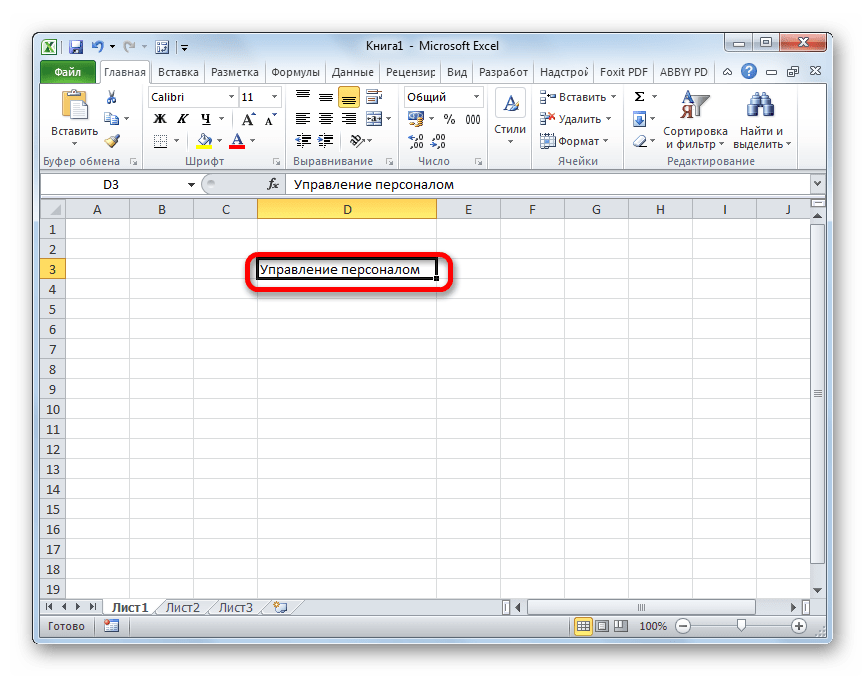
Текстовый тип содержит символьные данные и не рассматривается Excel, как объект математических вычислений. Это информация в первую очередь для пользователя, а не для программы. Текстом могут являться любые символы, включая цифры, если они соответствующим образом отформатированы. В языке DAX этот вид данных относится к строчным значениям. Максимальная длина текста составляет 268435456 символов в одной ячейке.
Для ввода символьного выражения нужно выделить ячейку текстового или общего формата, в которой оно будет храниться, и набрать текст с клавиатуры. Если длина текстового выражения выходит за визуальные границы ячейки, то оно накладывается поверх соседних, хотя физически продолжает храниться в исходной ячейке.
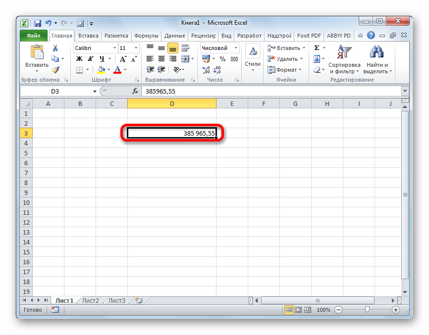
Числовые данные
Для непосредственных вычислений используются числовые данные. Именно с ними Excel предпринимает различные математические операции (сложение, вычитание, умножение, деление, возведение в степень, извлечение корня и т.д.). Этот тип данных предназначен исключительно для записи чисел, но может содержать и вспомогательные символы (%, $ и др.). В отношении его можно использовать несколько видов форматов:
- Собственно числовой;
- Процентный;
- Денежный;
- Финансовый;
- Дробный;
- Экспоненциальный.
Кроме того, в Excel имеется возможность разбивать числа на разряды, и определять количество цифр после запятой (в дробных числах).
Ввод числовых данных производится таким же способом, как и текстовых значений, о которых мы говорили выше.
Дата и время
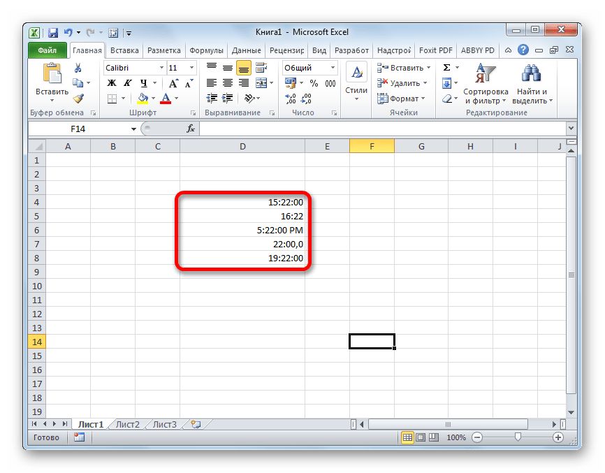
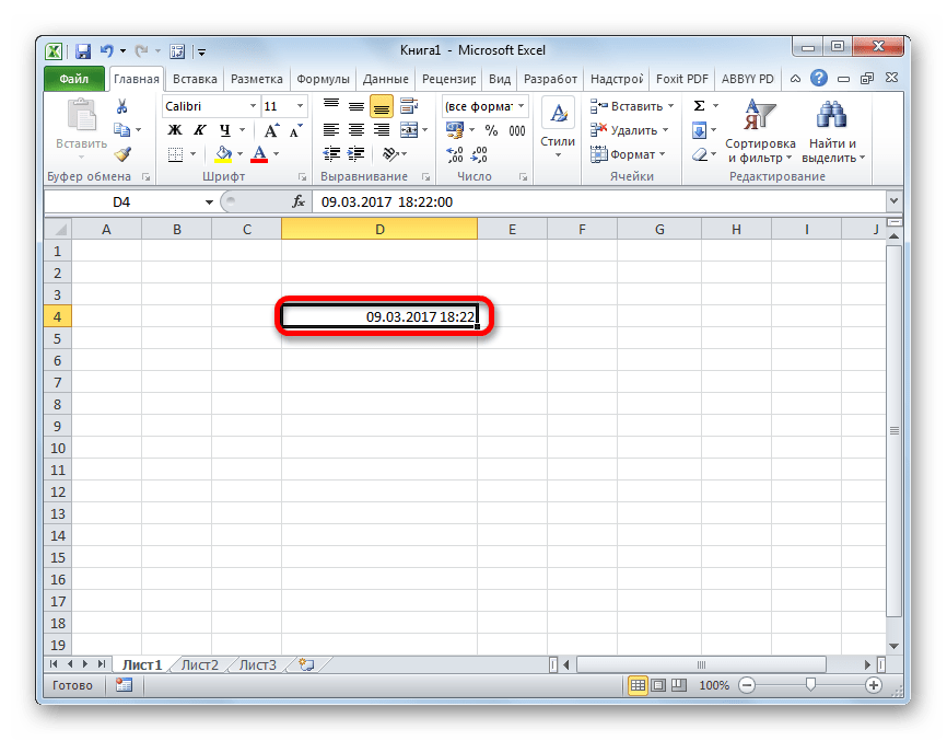
Ещё одним типом данных является формат времени и даты. Это как раз тот случай, когда типы данных и форматы совпадают. Он характеризуется тем, что с его помощью можно указывать на листе и проводить расчеты с датами и временем. Примечательно, что при вычислениях этот тип данных принимает сутки за единицу. Причем это касается не только дат, но и времени. Например, 12:30 рассматривается программой, как 0,52083 суток, а уже потом выводится в ячейку в привычном для пользователя виде.

Существует несколько видов форматирования для времени:
- ч:мм:сс;
- ч:мм;
- ч:мм:сс AM/PM;
- ч:мм AM/PM и др.
Аналогичная ситуация обстоит и с датами:
- ДД.ММ.ГГГГ;
- ДД.МММ
- МММ.ГГ и др.
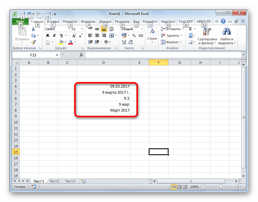
Есть и комбинированные форматы даты и времени, например ДД:ММ:ГГГГ ч:мм.
Также нужно учесть, что программа отображает как даты только значения, начиная с 01.01.1900.
Урок: Как перевести часы в минуты в Excel
Логические данные
Довольно интересным является тип логических данных. Он оперирует всего двумя значениями: «ИСТИНА» и «ЛОЖЬ». Если утрировать, то это означает «событие настало» и «событие не настало». Функции, обрабатывая содержимое ячеек, которые содержат логические данные, производят те или иные вычисления.

Ошибочные значения
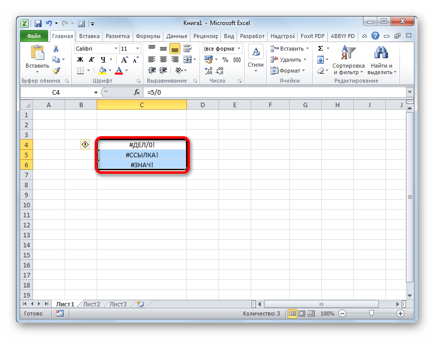
Отдельным типом данных являются ошибочные значения. В большинстве случаев они появляются, когда производится некорректная операция. Например, к таким некорректным операциям относится деление на ноль или введение функции без соблюдения её синтаксиса. Среди ошибочных значений выделяют следующие:
- #ЗНАЧ! – применение неправильного вида аргумента для функции;
- #ДЕЛ/О! – деление на 0;
- #ЧИСЛО! – некорректные числовые данные;
- #Н/Д – введено недоступное значение;
- #ИМЯ? – ошибочное имя в формуле;
- #ПУСТО! – некорректное введение адресов диапазонов;
- #ССЫЛКА! – возникает при удалении ячеек, на которые ранее ссылалась формула.
Формулы
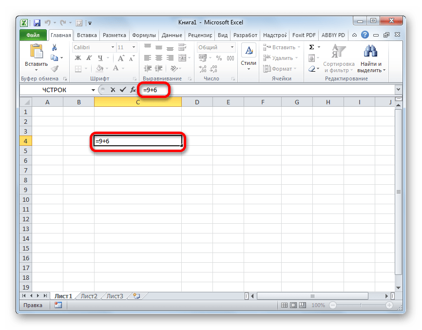
Отдельной большой группой видов данных являются формулы. В отличие от констант, они, чаще всего, сами не видны в ячейках, а только выводят результат, который может меняться, в зависимости от изменения аргументов. В частности, формулы применяются для различных математических вычислений. Саму формулу можно увидеть в строке формул, выделив ту ячейку, в которой она содержится.

Обязательным условием, чтобы программа воспринимала выражение, как формулу, является наличие перед ним знака равно (=).
Формулы могут содержать в себе ссылки на другие ячейки, но это не обязательное условие.
Отдельным видом формул являются функции. Это своеобразные подпрограммы, которые содержат установленный набор аргументов и обрабатывают их по определенному алгоритму. Функции можно вводить вручную в ячейку, поставив в ней предварительно знак «=», а можно использовать для этих целей специальную графическую оболочку Мастер функций, который содержит весь перечень доступных в программе операторов, разбитых на категории.
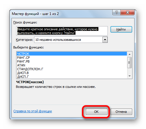
С помощью Мастера функций можно совершить переход к окну аргумента конкретного оператора. В его поля вводятся данные или ссылки на ячейки, в которых эти данные содержатся. После нажатия на кнопку «OK» происходит выполнение заданной операции.

Урок: Работа с формулами в Excel
Урок: Мастер функций в Excel
Как видим, в программе Excel существует две основные группы типов данных: константы и формулы. Они, в свою очередь делятся, на множество других видов. Каждый тип данных имеет свои свойства, с учетом которых программа обрабатывает их. Овладение умением распознавать и правильно работать с различными типами данных – это первоочередная задача любого пользователя, который желает научиться эффективно использовать Эксель по назначению.
Asked
10 years, 1 month ago
Viewed
13k times
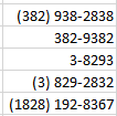
Is there any way in which I can predefine data type of a column of an excel sheet ?
For eg. when I enter 0022598741 in a column it will be formatted as 22598741 but I want it as it is.In this case this particular column takes the data as number type but I want it to be taken as text type.
- excel
asked Feb 19, 2013 at 14:19
![]()
SharmiSharmi
791 gold badge1 silver badge10 bronze badges
2
-
As this question stands, it will be a better fit over on SuperUser.
Feb 19, 2013 at 14:22
-
@Buggabill already flagged to move.
Feb 19, 2013 at 14:22
1 Answer
Format it as Text before input: right click > cell properties.
answered Feb 19, 2013 at 14:22
![]()
Peter L.Peter L.
7,2465 gold badges34 silver badges53 bronze badges
2
-
Actually I need to predefine the column type before hand and then it will be downloaded somewhere else and used. So will «right click > cell properties» work in that case ?
Feb 19, 2013 at 14:26
-
For sure and that’s the best way to preserve input: select entire column, format as text, save the file and send wherever you need -format will be kept.
Feb 19, 2013 at 14:27
- The Overflow Blog
- Featured on Meta
Related
Hot Network Questions
-
The Dating Game / Secretary Problem
-
Looking for a 90’s sorcery game on Atari ST
-
Sheet music shown in Picard S3 end credits: what song is this?
-
For the purposes of the Regenerate spell, does a snail shell count as a limb?
-
A Question on the Proof of A Form of the Minkowski Inequality
-
What’s the meaning of «Mek» from the Gentleman «Red town» song?
-
What remedies can a witness use to satisfy the «all the truth» portion of his oath?
-
Salvage tuna marinated in pineapple
-
Antonym for “elitist” with a negative connotation?
-
How do I create BLeeM’s «Emphasis Rolls» on Anydice?
-
How would a future humanity «terraform» the moon?
-
Gödel encoding — Part I
-
Is it okay to hard-code table and column names in queries?
-
Why are accessible states taken as eigenstates in statistical physics? Is the resolution via decoherence?
-
What’s the name of the piece that holds the fender on (pic attached)
-
What additional inputs are required to convert dBFS to dB SPL?
-
touch command not able to create file in write-permitted directory
-
What is the difference between elementary and non-elementary proofs of the Prime Number Theorem?
-
Is there a way to sign a transaction?
-
How can one transform a neutral lookup table texture for color blindness?
-
«Why» do animals excrete excess nitrogen instead of recycling it?
-
compare software available for Debian stable vs Ubuntu LTS (to work with data)
-
Inconsistent kerning in units when using detect-all
-
Division of binary numbers, confusing
more hot questions
Question feed
Your privacy
By clicking “Accept all cookies”, you agree Stack Exchange can store cookies on your device and disclose information in accordance with our Cookie Policy.
This tutorial about cell format types in Excel is an essential part of your learning of Excel and will definitely do a lot of good to you in your future use of this software, as a lot of tasks in Excel sheets are based on cells format, as well as several errors are due to a bad implementation of it.
A good comprehension of the cell format types will build your knowledge on a solid basis to master Excel basics and will considerably save you time and effort when any related issue occurs.
A- Introduction
Excel software formats the cells depending on what type of information they contain.
To update the format of the highlighted cell, go to the “Home” tab of the ribbon and click, in the “Number” group of commands on the “Number Format” drop-down list.
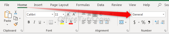
The drop-down list allows the selection to be changed.
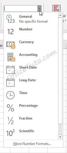
Cell formatting options in the “Number Format” drop-down list are:
- General
- Number
- Currency
- Accounting
- Short Date
- Long Date
- Time
- Percentage
- Fraction
- Scientific
- Text
- And the “More Number Formats” option.
Clicking the “More Number Formats” option brings up additional options for formatting cells, including the ability to do special and custom formatting options.
These options are discussed in detail in the below sections.
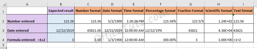
Cell format types in Excel are: General, Number, Currency, Accounting, Date, Time, Percentage, Fraction, Scientific, Text, Special (Zip Code, Zip Code + 4, Phone Number, Social Security Number), and Custom. You can get them from the “Number Format” drop-down list in the “Home” tab, or from the launcher arrow below it.
I will detail each one of them in the following sections:
1- General format
By default, cells are formatted as “General”, which could store any type of information. The General format means that no specific format is applied to the selected cell.
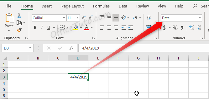
When information is typed into a cell, the cell format may change automatically. For example, if I enter “4/4/19” into a cell and press enter, then highlight the cell to view details about it, the cell format will be listed as “Date” instead of “General”.
Similarly, we can update a cell’s format before or after entering data to adjust the way the data appears. Changing the format of a cell to “Currency” will make it so information entered is displayed as a dollar amount.
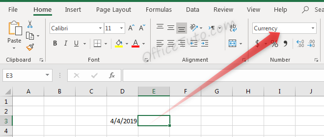
Typing a number into this cell and pressing enter will not just show that number, but will instead format it accordingly.
Before pressing enter, Excel shows the value which was typed: “4”.
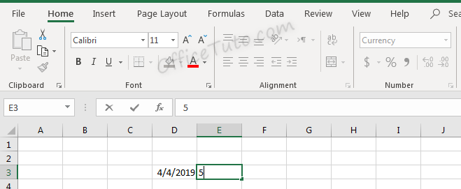
After pressing enter, the value is updated based on the formatting type selected.
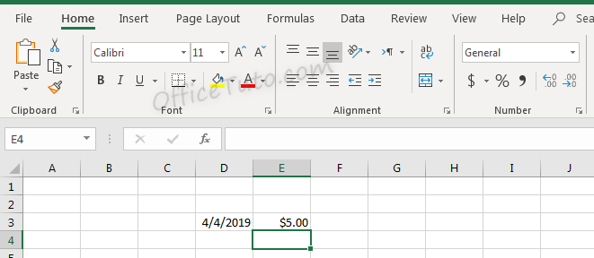
Don’t let the format type showed in the illustration at the drop-down list confusing you; it is reflecting the cell below (i.e. E4), since we validated by an Enter.
2- Number format
Cells formatted as numbers behave differently than general formatted cells. By default, when a number is entered, or when a cell is formatted as a number already, the alignment of the information within the cell will be on the right instead of on the left. This makes it easier to read a list of numbers such as the below.
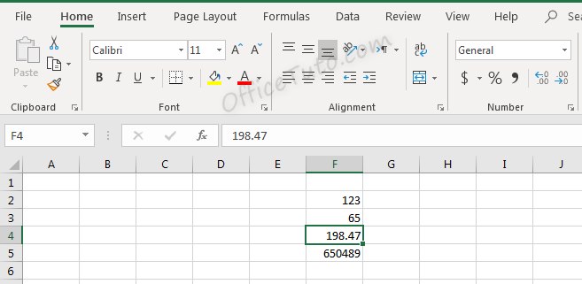
Note in the above screenshot that since we didn’t choose the “Number” format for our cells, they still have a “General” one. They are numbers for Excel (meaning, we can do calculations on them), but they didn’t have yet the number format and its formatting aspects:
You can set the formatting options for Excel numbers in the “Format Cells” dialog box.
To do that, select the cell or the range of cells you want to set the formatting options for their numbers, and go to the “Home” tab of the ribbon, then in the “Number” group of commands, click on the launcher of the dialog box (the arrow on the right-down side of the group).
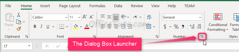
Excel opens the “Format Cells” dialog box in its “Number” tab. Click in the “Category” pane on “Number”.
- In this dialog box, you can decide how many decimal places to display by updating options in the “Decimal places” field.
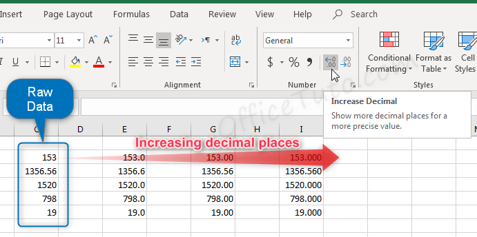
Note that this feature is also available in the “Home” tab of the ribbon where you can go to the “Number” group of commands and click the Increase Decimal ![]() or Decrease Decimal
or Decrease Decimal ![]() buttons.
buttons.
Here is the result of consecutive increasing of decimal places on our example of data (1 decimal; 2 decimals; and 3 decimals):
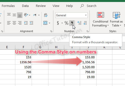
- You can also decide if commas should be shown in the display as a thousand separator, by updating the “Use 1000 Separator (,)” option in the “Format Cells” dialog box.
This feature is also available in the “Home” tab of the ribbon by clicking the “Comma Style” button ![]() in the “Number” group of commands.
in the “Number” group of commands.
Note that using the Comma Style button will automatically set the format to Accounting.
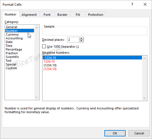
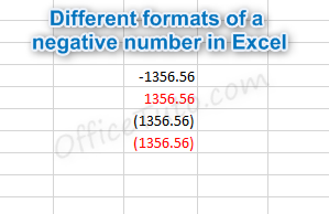
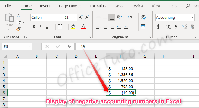
- Another option from the Format Cells dialog box is to decide how negative numbers should display by using the “Negative numbers” field.
There are four options for displaying negative
numbers.
- Display
negative numbers with a negative sign before the number. - Display
negative numbers in red. - Display
negative numbers in parentheses. - Display
negative numbers in red and in parentheses.
3- Currency format
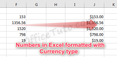
Cells formatted as currency have a currency symbol such as a dollar sign $ immediately to the left of the number in the cell, and contain two numbers after the decimal by default.
The alignment of numbers in currency formatted cells will be on the right for readability.
Currency formatting options are similar to
number formatting options, apart from the currency symbol display.
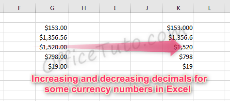
- As with regular number formatting, you can decide, in the “Format Cells” dialog box, how many decimal places to display by updating the field “Decimal places”.
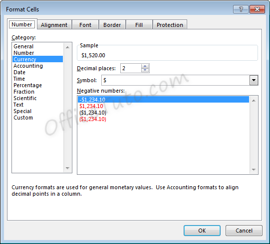
You can also find this feature in the “Home” tab of the ribbon, by going to the “Number” group of commands and clicking the Increase Decimal ![]() or Decrease Decimal
or Decrease Decimal ![]() .
.
- You can also decide what currency symbol should be shown in the display by updating the “Symbol” field in the “Format Cells” dialog box.
- As with regular number formatting, you can also decide how negative numbers should display by updating the “Negative numbers” field in the “Format Cells” dialog box.
There are four
options for displaying negative numbers.
- Display
negative numbers with a negative sign before the number. - Display
negative numbers in red. - Display
negative numbers in parentheses. - Display
negative numbers in red and in parentheses.
4- Accounting format
Like with the currency format, cells formatted as accounting have a currency symbol such as a dollar sign $; however, this symbol is to the far left of the cell, while the alignment of numbers in the cell is on the right. Accounting numbers contain two numbers after the decimal by default.
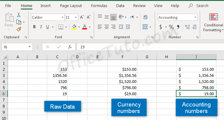
Clicking the “Accounting Number Format” button ![]() in the “Number” group of commands of the “Home” tab, will quickly format a cell or cells as Accounting.
in the “Number” group of commands of the “Home” tab, will quickly format a cell or cells as Accounting.
The down arrow to the right of the Accounting Number Format button allows selection between common symbols used for accounting, including English (dollar sign), English (pound), Euro, Chinese, and French symbols.
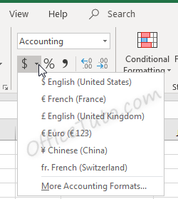
Accounting formatting options in the “Format Cells” dialog box (“Home” tab of the ribbon, in the “Number” group of commands, click on the launcher of the “Number Format” dialog box), are similar to number and currency formatting options.
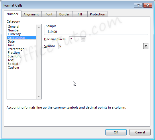
- You can decide how many decimal places to display by updating its option in the “Format Cells” dialog box.
As mentioned before in this tutorial, this feature is also available directly in the “Home” tab of the ribbon by clicking the Increase Decimal ![]() or Decrease Decimal
or Decrease Decimal ![]() buttons in the “Number” group of commands.
buttons in the “Number” group of commands.
- You can also decide in the “Format Cells” dialog box, what currency symbol should be shown in the display by using the “Symbol” drop-down list.
This dropdown gives a much broader list of options than the “Accounting Number Format” option in the “Home” tab of the ribbon.
Note that with the Accounting formatting option, negative numbers display in parentheses by default. There are not options to change this.
5- Date format
There are options for “Short Date” and “Long Date” in the “Number Format” dropdown list of the “Home” tab.
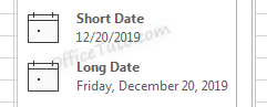
Short date shows the date with slashes separating month, day, and year. The order of the month and day may vary depending on your computer’s location settings.
Long date shows the date with the day of the week, month, day, and year separated by commas.
More options for formatting dates are available in the “Format Cells” dialog box (accessible by clicking in the “Number Format” dropdown list of the “Home” tab and choosing the “More Number Formats” option at the bottom).
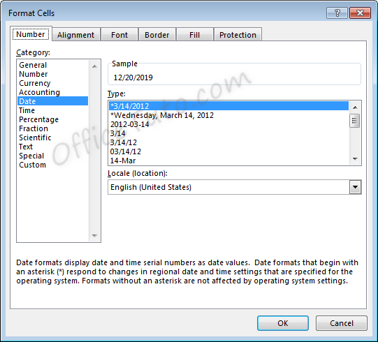
- You can choose from a long list of available date formats.
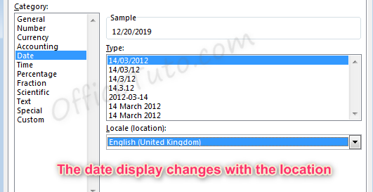
- You can update the location settings used for formatting the date. This will alter the list of format options in the above list and will adjust the display and potentially the order of the elements (day, month, year) within the date.
Note the below example when we switch from English (United States) format to English (United Kingdom) format.
6- Time format
Cells formatted as time display the time of
day. The default time display is based on your computer’s location settings.
Time formatting options are available in the “Format Cells” dialog box (accessible by choosing the “More Number Formats” option at the bottom of the “Number Format” dropdown list in the “Home” tab of the ribbon).
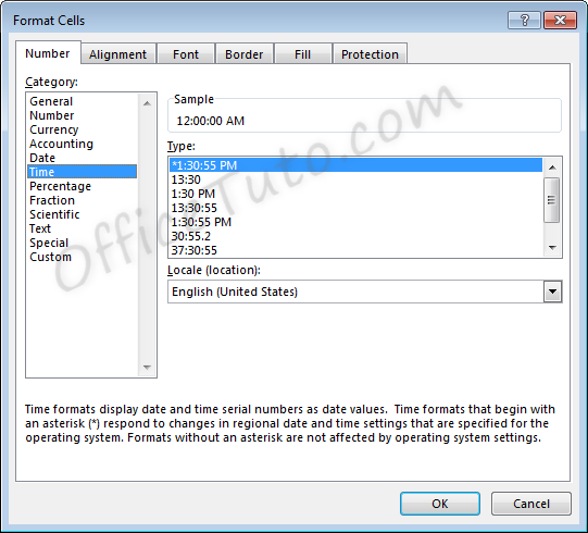
- You can choose from a long list of available time formats.
- You can update the location settings used for formatting the time. This will alter the list of format options in the above list and will adjust the display.
7- Percentage format
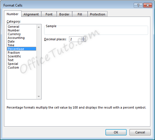
Cells formatted as percentage display a percent sign to the right of the number. You can change the format of a cell to a percentage using the “Number Format” dropdown list, or by clicking the “Percent Style” button ![]() . Both options are accessible from the “Home” tab of the ribbon, in the “Number” group of commands.
. Both options are accessible from the “Home” tab of the ribbon, in the “Number” group of commands.
Note that updating a number to a percentage
will expect that the number already contains the decimal. For example:
A cell containing the value 0.08, as a percentage, will show 8%.
A cell containing the value 8, as a percentage, will show 800%.
Percentage formatting options are available in the “Format Cells” dialog box, accessible by clicking on “More Number Formats” of the “Number Format” dropdown list in the “Home” tab of the ribbon.
8- Fraction format
Cells formatted as a fraction display with a slash
symbol separating the numerator and denominator.
Fraction formatting options are available in the “Format Cells” dialog box, accessible by clicking in the “Home” tab of the ribbon, on “More Number Formats” of the “Number Format” dropdown list.
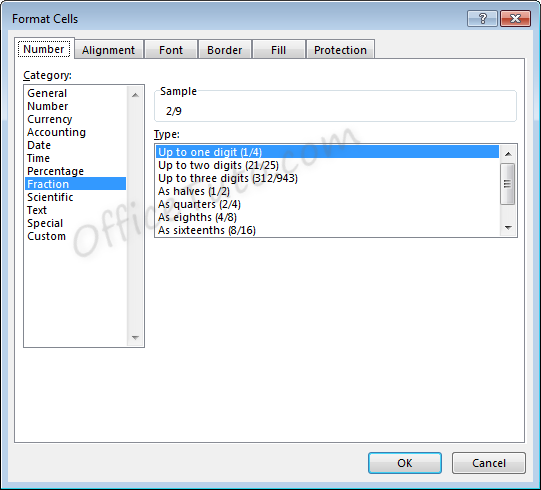
- Note that
when selecting the format to use for a fraction, Excel will round to the
nearest fraction where the formatting criteria can be met.
As an example, if the
formatting option selected is “Up to one digit”, entering a fraction with two
digits will cause rounding to occur. For example, with the setting of “Up to
one digit”,
If we enter a value of 7/16, the value displayed will be 4/9, as converting to 9ths was the option with only one digit which required the least amount of rounding.
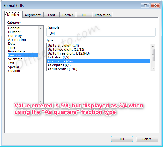
For another example, if the formatting option selected is “As quarters”, entering a fraction that cannot be expressed in quarters (divisible by four) will also cause rounding to occur.
If we enter a value of 5/8, the value displayed will be 3/4. Excel rounded up to 6/8, or 3/4, which was the closest option divisible by four.
- Also note
that for the formatting options with “Up to x digits”, Excel will always round
down to the lowest exact equivalent fraction when possible.
For example, if we enter a value of 2/4 with one of these formatting options active, the value displayed will be 1/2, as this is the mathematical equivalent. This behavior will not take place for formatting options “As…”, since these specifically determine what the denominator should be.
- Fractions listed as more than a whole (meaning the numerator is a higher number than the denominator), such as 7/4 will automatically be adjusted into a whole number and a fraction 13/4, where the fraction follows the formatting rules selected.
9- Scientific format
Scientific format, otherwise known as
Exponential Notation, allows very large and small numbers to be accurately
represented within a cell, even when the size of the cell cannot accommodate
the size of the numbers.
The way exponential notation works is to theoretically place a decimal in a spot that would make the number shorter, then describe where to move that decimal to return to the original number.
Examples with large numbers, where the decimal is moved to the left:
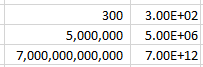
For the number 300 to be expressed in
exponential notation, Excel moves the decimal from after the whole number
300.00 to between the 3 and the 00. This is typed out as E+02 since the decimal
was moved two places to the left. The other examples are similar, where the
decimal was moved 6 and 12 places to the left.
Examples with small numbers, where the decimal is moved to the right:
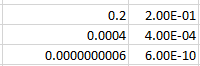
For the number 0.2 to be expressed in
exponential notation, Excel moves the decimal to create a whole number 2. This
is typed out as E-01 since the decimal was moved one place to the right. The
other examples are similar, where the decimal was moved 4 and 10 places to the
right.
Scientific formatting options are listed in the “Format Cells” dialog box, accessible by going to the “Home” tab of the ribbon, and clicking the “More Number Formats” option of the “Number Format” dropdown list.
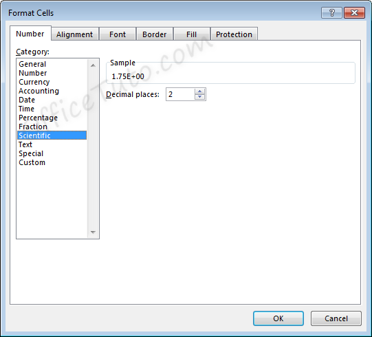
The only option available is to alter the
number of decimal places shown in the number prior to the scientific notation.
For example, for the value 11.43 formatted with the scientific format, if we change the Decimal places from 2 to 1, the display will change as follows.
Two decimals: 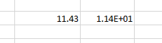
One decimal: 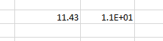
10- Text format
Cells can be formatted as Text through the
“Number Format” dropdown list, in the “Number” group of commands of the “Home”
tab.
Using the Text format in Excel allows values to be entered as they are, without Excel changing them per the above formatting rules.
In general, when entering a text in a cell, you won’t need to set its type to “Text”, as the default format type “General” is sufficient in most cases.
This may be useful when you want to display numbers with leading zeros, want to have spaces before or after numbers or letters, or when you want to display symbols that Excel normally uses for formulas.
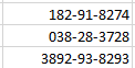
Below are examples of some fields formatted as Text.
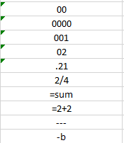
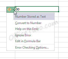
Note that when a number is formatted as Text, Excel will display a symbol showing that there could be a possible error ![]() .
.
Clicking the cell, then clicking the pop-up icon will show what the error may be and offer suggestions for resolution.
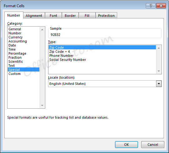
11- Special format
Special format offers four options in the “Format Cells” dialog box, accessible by going to the “Home” tab of the ribbon, and clicking the launcher arrow in the “Number” group of commands.
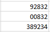
- Zip Code
When less than five numbers are entered in Zip
Code format, leading zeros will be added to bring the total to five numbers.
When more than five numbers are entered in Zip Code format, all numbers will be displayed, even though this does not meet the format criteria.
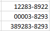
- Zip Code + 4
Zip Code + 4 format automatically creates a
dash symbol – before the last four numbers in the zip code.
When less than nine numbers are entered in Zip
Code + 4 format, leading zeros will be added to bring the total to nine
numbers.
When more than nine numbers are entered in Zip Code + 4 format, extra numbers are displayed prior to the dash symbol –.
- Phone Number
Phone Number format automatically creates a
dash –
before the last four numbers in the phone number. This format also adds
parentheses ( ) around the area code when an area code is entered.
When less than the expected number of digits
are entered in Phone Number format, only the entered digits will be displayed,
starting from the end of the phone number, as shown on the third and fourth
lines, below.
When more than the expected number of digits
are entered in Phone Number format, extra numbers are displayed within the area
code parentheses.
Note that Phone Number format in Excel does not handle the number 1 before an area code. This entry would be treated like any other extra number.
- Social Security Number
Social Security Number format automatically
creates a dash – before the last four numbers in the social security number
and a dash before the last six numbers in the social security number.
When less than nine numbers are entered in
Social Security Number format, leading zeros will be added to bring the total
to nine numbers.
When more than nine numbers are entered in Social Security Number format, extra numbers are displayed prior to the first dash –.
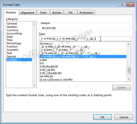
12- Custom format
Custom formats can be used or added through the
“Format Cells” dialog box, accessible from the “Number” group of commands in
the “Home” tab of the ribbon by clicking the “Number Format” launcher arrow.
This can be useful if the above formatting options do not work for your needs. Custom number formats can be created or updated by typing into the “Type” field of the “Format Cells” dialog box.
When creating a new custom format, be sure to use an existing custom format that you are okay with changing.
Custom number formats are separated, at
maximum, into four parts separated by semicolons ; .
- Part 1: How
to handle positive number values - Part 2: How
to handle negative number values - Part 3: How
to handle zero number values - Part 4: How
to handle text values
Note that if fewer parts are included in the custom format coding, Excel will determine how best to merge the above options: As an example, if two parts are listed, positive and zero values will be grouped.
Note that Excel may update the formatting of some fields to Custom automatically depending on what actions are taken on the field.
C- Common issues caused by wrong cell format types in Excel
1- Common issues due to wrong cell format types in Excel
The most common problems you may encounter with a wrong cell format type in Excel are of 3 types:
– Getting a wrong value.
– Getting an error.
– Formula displayed as-is and not calculated.
Let’s illustrate these 3 cases with some examples:
- Getting a wrong value
This may occur when you enter a value in an already formatted cell with an inappropriate format type, or when you apply a different format to a cell already containing a value.
The following table details some examples:
- Getting an error
This occurs when you enter a text preceded with a symbol of a dash, or plus, or equal, as an element of a list.
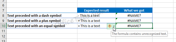
Excel wrongly interprets the text as a formula and show the error “The formula contains unrecognized text”.
- Formula displayed as-is and not calculated
In the following example, we tried to calculate the total of prices from cell B2 to B6 using the Excel SUM function, but Excel doesn’t calculate our formula and just displayed it as-is.
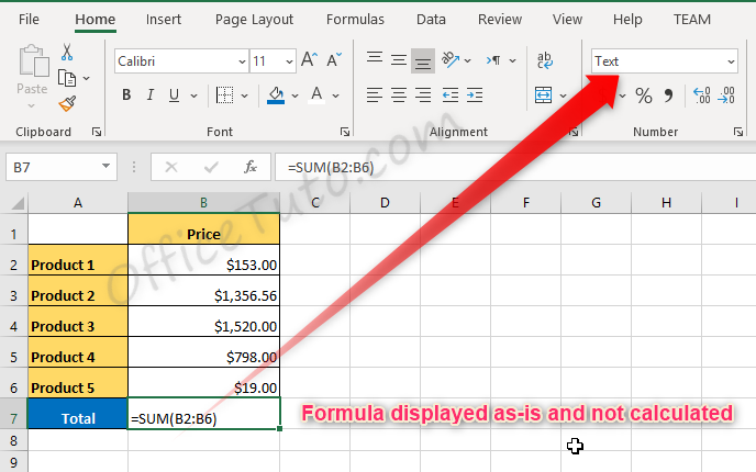
The source of the problem is that the result cell, B7, was previously formatted as text before entering the formula.
2- How to correct wrong cell format type issues in Excel
To correct cell format type issues in Excel, apply the right format in the “Number Format” drop-down list, and sometimes, you’ll also need to re-enter the content of the cell. For cells with formulas displayed as text, choose the “General” format, then double click in the cell and press Enter.

Jeff Golden is an experienced IT specialist and web publisher that has worked in the IT industry since 2010, with a focus on Office applications.
On this website, Jeff shares his insights and expertise on the different Office applications, especially Word and Excel.