
Range.EntireColumn
Yes! You can use Range.EntireColumn MSDN
dim column : column = 4

dim column_range : set column_range = Sheets(1).Cells(column).EntireColumn
Range(«ColumnName:ColumnName»)
If you were after a specific column, you could create a hard coded column range with the syntax e.g. Range("D:D").
However, I’d use entire column as it provides more flexibility to change that column at a later time.
Worksheet.Columns
Worksheet.Columns provides Range access to a column within a worksheet. MSDN
If you would like access to the first column of the first sheet. You would
call the Columns function on the worksheet.
dim column_range: set column_range = Sheets(1).Columns(1)
The Columns property is also available on any Range MSDN
EntireRow can also be useful if you have a range for a single cell but would like to reach other cells on the row, akin to a LOOKUP
dim id : id = 12345


dim found : set found = Range("A:A").Find(id)

if not found is Nothing then
    'Get the fourth cell from the match
    MsgBox found.EntireRow.Cells(4)
end if
When given a single cell reference, the COLUMN function returns the column number for that reference. However, when given a range that contains multiple columns, the COLUMN function will return an array that contains all column numbers for the range. In the example shown the array looks like this:
{2,3,4}
If you want only the first column number, you can use the MIN function to extract just the first column number, which will be the lowest number in the array.
Simple version
Entered in a single cell, the COLUMN function will display only the first column number, even when it returns an array. This means, in practice, you can often just use the COLUMN function alone:
=COLUMN(rng)
However, inside formulas more complex formulas, it’s sometimes necessary to make sure you are dealing with only one item, and not an array. In that case, you’ll want to use MIN to pull out just the first item.
We can get a complete set of relative column numbers in a range with an array formula that is based on the COLUMN function. The steps below will walk through the process.
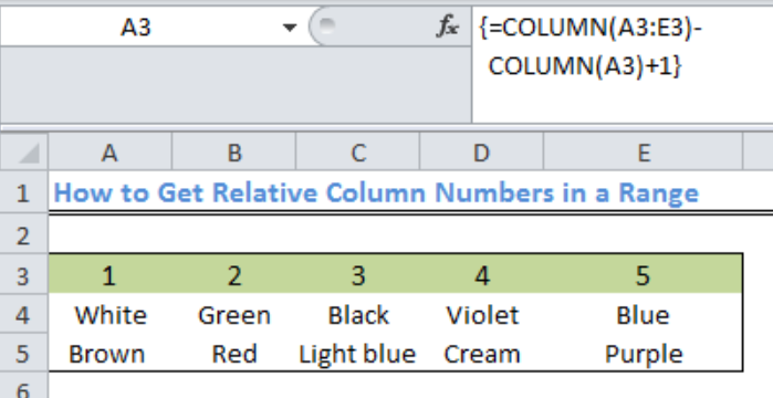 Figure 1: Result of Relative Column Numbers in a Range:
General Formula
{=COLUMN(range)-COLUMN(firstcell)+1}
Formula
=COLUMN(A3:E3)-COLUMN(A3)+1
Setting up the Data
We will determine the relative column number for range A3:E3 based on the content of figure 2
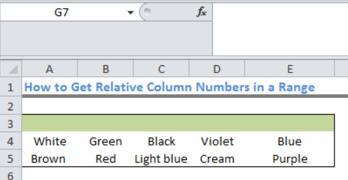 Figure 2: Setting up the Data
Get Relative Column Numbers in a Range
- We will highlight the range from Cell A3 to E3
- We will input the formula below inside the range
{=COLUMN(A3:E3)-COLUMN(A3)+1}
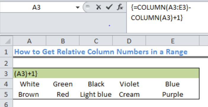 Figure 3: How to Get Relative Column Numbers in a Range
- Because this is an array formula, we will press CTRL+SHIFT+ENTER to get the result
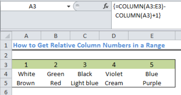 Figure 4: Result of Relative Column Numbers in a Range
Explanation
In this formula, the first Column function creates an array of 5 numbers like this: {2,3,4,5,6}. The second Column function creates an array that has only one item: {2}. This is subtracted from the first array and results in {0,1,2,3,4}. 1 is added to the result to produce: {1,2,3,4,5}.
Instant Connection to an Expert through our Excelchat Service
Most of the time, the problem you will need to solve will be more complex than a simple application of a formula or function. If you want to save hours of research and frustration, try our live Excelchat service! Our Excel Experts are available 24/7 to answer any Excel question you may have. We guarantee a connection within 30 seconds and a customized solution within 20 minutes.
-
Select the cell where you want the result to appear.
-
On the Formulas tab, click More Functions, point to Statistical, and then click one of the following functions:
-
COUNTA: To count cells that are not empty
-
COUNT: To count cells that contain numbers.
-
COUNTBLANK: To count cells that are blank.
-
COUNTIF: To count cells that meets a specified criteria.
Tip: To enter more than one criterion, use the COUNTIFS function instead.
-
-
Select the range of cells that you want, and then press RETURN.
-
Select the cell where you want the result to appear.
-
On the Formulas tab, click Insert, point to Statistical, and then click one of the following functions:
-
COUNTA: To count cells that are not empty
-
COUNT: To count cells that contain numbers.
-
COUNTBLANK: To count cells that are blank.
-
COUNTIF: To count cells that meets a specified criteria.
Tip: To enter more than one criterion, use the COUNTIFS function instead.
-
-
Select the range of cells that you want, and then press RETURN.
I’m going to start by reviewing a couple fundamentals about selecting ranges in Excel with VBA, then I’ll discuss methods for selecting ranges with variable row numbers.
Selecting Cells in Excel
One of the most common situations in Microsoft Excel is that you need to select a cell or a range of cells to perform an action. For example, even just to copy and paste content, you need to perform steps below one-by-one (I bet you never thought this was actually a complex task).
- Select the cell(s) to be copied
- Click on copy (or) ctrl + c
- Select the cell(s) into which the content needs to be pasted
- Click on paste (or) ctrl + v
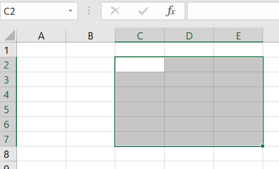
In this process, we select one cell or multiple cells that are in continuous rows and columns. This continuous selection is called a “Range”. A range is generally identified by the starting cell reference in the left-side top corner and ending cell reference in the bottom right corner of the selection. For example, in the image below, the range is from C2 to E7. All the cells within this cell reference are selected.
The Range Expression
VBA offers a Range expression that can be used in selection of cells.
Syntax:
Range (“ < reference starting cell > : < reference ending cell >”)
(or)
Range ( Cells ( <row_number> , <col_number> ) , Cells ( <row_number> , <col_number> ) )
In other words, the range of cells selected in the image above can be expressed in any one of the following ways — for our example, we’ll assume that we are selecting the range on a sheet named “Wonders.”
Sheets("Wonders").Range("C2:E7").Select
Note that letters are used to represent column number and row is indicated by a number. There is a colon in between to two cell references and the entire parameter is encased in double quotes.
Sheets("Wonders").Range(Cells(2, 3), Cells(7, 5)).Select
In this case, double quotes are not used for the range. There is comma instead of the colon symbol, and the cell references are represented using the Cells expression and the row and column numbers.
Try it yourself. Name an Excel sheet “Wonders.” Try running the code below and check the “Wonders” sheet to see what has been selected.
Sub range_demo()
Sheets("Wonders").Range("B2:F6").Select
Sheets("Wonders").Range(Cells(2, 3), Cells(7, 5)).Select
End Sub
Variable row numbers in the Range expression
So far we’ve tried to select a range of cells knowing the exact references of two cells that form the range. Now, it is time to see how to insert a dynamic or varying row or column number in the same expression.
The way to do it is simply with concatenation using double quotes and the ampersand (&) symbol.
Let’s look at some examples.
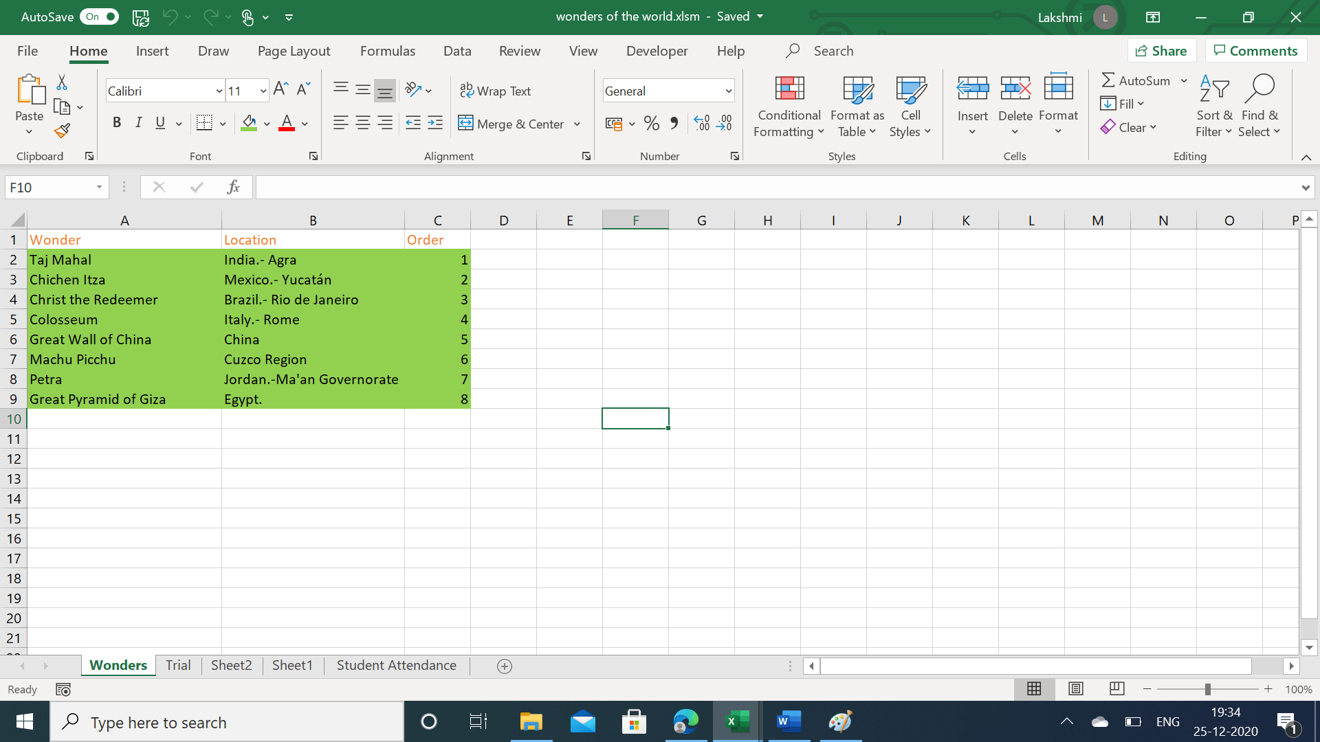
Color a range of cells up to a dynamically changing last row
In the example below, let’s find the last used row and dynamically use that row in the Range expression. This example will color the selected cells in green.
Sub range_demo()
'declare variable
Dim lastrow As Integer
'initialize variable
lastrow = ActiveSheet.UsedRange.Rows.Count
'Use the variable in the range expression to select
Sheets("Wonders").Range("A2:C" &amp;amp;amp; lastrow).Select
'colour the selected cells in green
With Selection.Interior
.Pattern = xlSolid
.PatternColorIndex = xlAutomatic
.Color = 5296274 'green colour
End With
End Sub
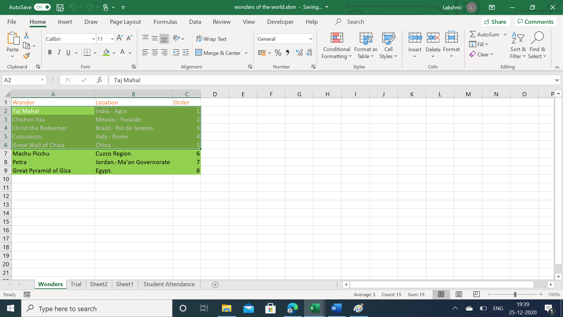
Color the font of selected cells up to a specific row input by the user
Below is another example that uses the Cells expression to do the same thing. Here we will change the font color of the selected cells.
Sub range_demo()

'declare variable
Dim row_num As Integer

'initialize variable - enter 6 while running the code
row_num = InputBox("Enter the row number")

'Use the variable in the range expression to select only the first 5 rows of data - not the headers
Sheets("Wonders").Range(Cells(2, 1), Cells(row_num, 3)).Select

'colour the font of selected cells in white
With Selection.Font
        .ThemeColor = xlThemeColorDark1
        .TintAndShade = 0
End With

End Sub
Use a different runtime number in both cell references
In this example, we’re still not hardcoding the cell references. Three rows starting from the row number input by the user are formatted in “Bold.”
Sub range_demo()

'declare variable
Dim row_num As Integer

'initialize variable - enter 3 while running the code
row_num = InputBox("Enter the row number")

'Use the variable in the range expression to select only the first 3 rows of data starting from the row_num input by the user
Sheets("Wonders").Range(Cells(row_num, 1), Cells((row_num + 3), 3)).Select

'make the font of the selected cells to "Bold"
Selection.Font.Bold = True

End Sub

Concatenating both cell references of a simple range expression
Sub range_demo()
'declare variable
Dim row_num As Integer
'initialize variable - enter 7 while running the code
row_num = InputBox("Enter the row number")
'Use the variable in the range expression to select only the first 3 rows of data starting from the row_num input by the user
Sheets("Wonders").Range("A" &amp;amp;amp; row_num &amp;amp;amp; ":C" &amp;amp;amp; row_num + 2).Select
'make the font of the selected cells to "Italics"
Selection.Font.Italic = True
End Sub

Conclusion
The Range expression in VBA is very useful for calculating and formatting cells in MS Excel. Not just row numbers, but also column numbers can be dynamically inserted to make the best use of the expression. In other words, instead of hard coding the reference directly, we can use a variable that holds the number in the expression.
Column Letter to Number in Excel
Figuring out which row you are in is as easy as you like. But, how do you tell which column you are in now? Excel has 16,384 columns, represented by alphabetic characters in Excel. So, suppose you want to find the column CP. How do you tell?
Yes, it is almost impossible to figure out the column number in Excel. However, nothing to worry about because we have a built-in function called COLUMN in excelColumn function finds out the column numbers of the target cells in excel. It takes one argument which is the target cell as reference. Note that this function does not give the value of the cell as it returns only the column number of the cell. read more, which can tell the exact column number we are in right now or find the column number of the supplied argument.
Table of contents
- Column Letter to Number in Excel
- How to Find Column Number in Excel? (with Examples)
- Example #1
- Example #2
- Example #3
- Example #4
- Things to Remember
- Recommended Articles
- How to Find Column Number in Excel? (with Examples)
How to Find Column Numbers in Excel? (with Examples)
You can download this Column to Number Excel template here – Column to Number Excel template
Example #1
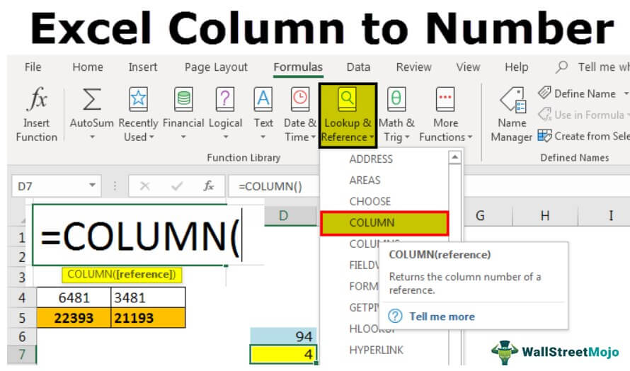
We can get the current column number by using the COLUMN function in Excel.
- We have opened a new workbook and typed some of the values in the worksheet.

- Let us say we are in cell D7, and we want to know the column number of this cell.

- To find the current column number, we must write the COLUMN function in the Excel cell and do not pass any argument; close the bracket.

- Press the “Enter” key. As a result, we will have a current column number in Excel.


Example #2
We can get the column number of the different cells by using the COLUMN function in Excel.
Getting the current column is not the toughest task at all. Suppose we want to know the column number of the cell CP5 and how we get that column number.
- We can write the COLUMN function and pass the specified cell value in any cells.

- Then press the “Enter” key. It will return the column number of CP5.

We have applied the COLUMN formula in cell D6 and passed the argument as CP5, i.e., cell referenceCell reference in excel is referring the other cells to a cell to use its values or properties. For instance, if we have data in cell A2 and want to use that in cell A1, use =A2 in cell A1, and this will copy the A2 value in A1.read more of CP5 cell. However, unlike normal cell reference, it will not return the value in the cell CP5. Rather, it will return the column number of CP5.
So, the column number of the cell CP5 is 94.
Example #3
We can get how many columns are selected in the range by using the COLUMNS function in Excel.
We have learned how to get the current cell column number and specified cell column number in Excel. But, how do you tell how many columns are selected in the range?
We have another built-in function called the COLUMNS function in excelThe COLUMNS function returns the total number of columns in the given array or collection of references.read more, which can return the number of columns selected in the formula range.
Assume we want to know how many columns are from the range C5 to N5.
- We can open the formula COLUMNS in any cell and select the range as C5 toN5.

- Press the “Enter” key to get the desired result.
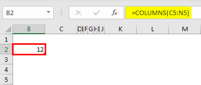
So totally, we have selected 12 columns in the range C5 to N5.
In this way, by using the COLUMN and COLUMNS function in Excel, we can get the two different kinds of results, which can help us calculate or identify the exact column when dealing with huge datasets.
Example #4
We can change the cell reference form to R1C1 references in Excel.
By default, we have cell references, all the rows are represented numerically, and all the columns are represented alphabetically.

It is the usual spreadsheet structure we are familiar with. The cell reference is started with the column alphabet and then followed by row numbers.
As we learned earlier in the article, we need to use the COLUMN function to get the column number. How about changing the column headers from the alphabet to numbers like our row headers? Like the image below.

It is called ROW-COLUMN reference in Excel. Now, take a look at the below image and the reference type.
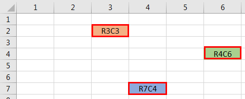
Unlike our standard cell reference, reference starts with a row number followed by a column number, not an alphabet.
Follow the below steps to change it to the R1C1 reference style.
- We must first go to the “File” and “Options.”

- Next, go to “Formulas” under “Options.”
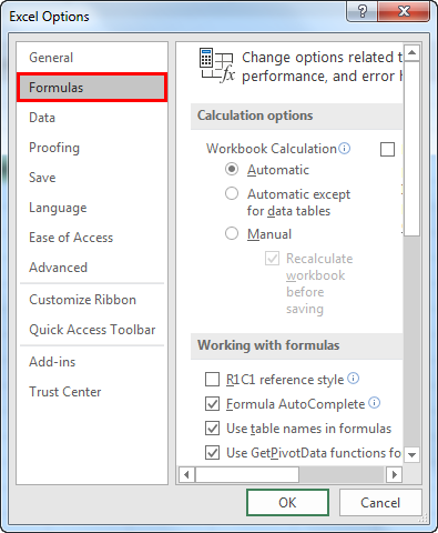
- Working with “Formulas,” select the checkbox “R1C1 reference style” and click “OK.”

Once we click “OK,” cells will change to R1C1 references.
Things to Remember
- The R1C1 cell reference is the rarely followed cell reference in Excel. As a result, we may get confused easily at the start.
- We see column alphabet first and row number next in normal cell references. But in R1C1 cell references, the row number will come first and the column number.
- The COLUMN function can return the current column number and the supplied column number.
- The R1C1 cell reference makes it easy to find the column number easily.
Recommended Articles
This article has been a guide to Column Letter to Numbers in Excel. We discuss finding column numbers in Excel using the COLUMN and COLUMNS functions. You may learn more about Excel from the following articles: –
- Excel Rows Function
- Excel Rows vs. Columns
- Excel Rows and Columns
- Concatenate Excel Columns
Excel COLUMNS Function (Example + Video)

When to use Excel COLUMNS Function
Excel COLUMNS function can be used when you want to get the number of columns in a specified range or array.
What it Returns
It returns a number that represents the total number of columns in the specified range or array.
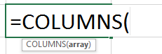
Syntax
=COLUMNS(array)
Input Arguments
- array – it could be an array, an array formula or a reference to a contiguous range of cells.
Additional Notes
- Even if the array contains multiple rows and columns, only the columns are counted. For example:
-
COLUMNS(A1:B1) returns 2.
-
COLUMNS(A1:B100) also returns 2.
-
- This formula can be useful when you want to get a sequence of numbers as you go to the right in your worksheet.
- For example, if you want 1 in A1, 2 in B1, 3 in C1 and so on, use the following formula =COLUMNS($A$1:A1). As you would drag this to the right, the reference inside it would change and the number of columns in the reference would get incremented by one. For example, when you drag it to column B1, the formula becomes COLUMNS($A$1:B1) which then returns 2.
Excel COLUMNS Function – Examples
Here are two examples of using the Excel COLUMNS function.
Example 1: Finding the number of Columns in an Array

In the example above, =COLUMNS(A1:A1) returns 1 as it covers one row (which is A1). Similarly, =COLUMNS(A1:C1) returns 3 as the array A1:C1 covers four columns in it.
Also, note that it only counts the number of columns. Hence, whether the array is A1:C1, or A1:C5, it would return 3 in both the cases.
Example 2: Getting a Sequence of Numbers in a Column

Excel COLUMNS function can be used to get a sequence of numbers. Since the first reference is fixed, as you copy the formula down, the second reference changes and so does the row numbers in the array.
Excel COLUMNS Function – Video Tutorial
Related Excel Functions:
- Excel COLUMN Function.
- Excel ROW Function.
- Excel ROWS Function
Other articles you may also like:
- Row vs Column in Excel – What’s the Difference?