
Facing problem just because your filter not working in Excel? No need to suffer from this problem anymore….!
As today I have chosen this specific topic of “Excel filter not working” to answer. All in all this post will help you to explore the reasons behind why Filter Function Not Working In Excel and ways to fix Excel filter not working issue.
Why Is Your Filter Not Working In Excel And Ways To Fix It?
Reason 1# Excel Filter Not Working With Blank Rows
One very common problem with the Excel filter function is that it won’t work with the blank rows. Excel Filter doesn’t count the cells with the first blank spaces.
To fix this, you need to choose the range right before using the filter function. For a clearer idea of how to perform this task, check out the following example.
- Before using the Excel filter function on the column C. either you can choose the column “C” completely or just select the data which you want to filter out.

- From the “data” tab select the “Filter” option. Now all the items become visible in the filter checkbox list or filtered list.
- Similarly, you have to choose the cell ranges or multiple columns before the application of the filter function.

To fix damaged Excel workbook, we recommend this tool:
This software will prevent Excel workbook data such as BI data, financial reports & other analytical information from corruption and data loss. With this software you can rebuild corrupt Excel files and restore every single visual representation & dataset to its original, intact state in 3 easy steps:
- Download Excel File Repair Tool rated Excellent by Softpedia, Softonic & CNET.
- Select the corrupt Excel file (XLS, XLSX) & click Repair to initiate the repair process.
- Preview the repaired files and click Save File to save the files at desired location.
Reason 2# Make Proper Selection Of The Data
If your spreadsheet contains empty rows or columns. Or if you only want to filter out only the specific range then choose the section which you want to filter prior to turning on the Filter.
If you don’t choose the area then Excel applies the filter on the complete one. This can also result in selection up to the first empty column or rows excluding the data present after the blanks.
So it will be better if you manually select the data in which you want to apply the Excel filter function.
- In order to remove the blank rows from the selected filter area. First of all turn on the filter and then click on the drop-down arrow present in any columns to show the filter list.
- Now remove the check sign across the ‘(Select All)’ after then shift right on the bottom of the filter list. Choose the ‘(Blanks)’ option and tap to the OK.

- After this only, the blank rows will clearly appear on your screen.
- For easy identification, the row number of each blank row appears in blue color.
- For deleting up these blank rows. You need to select these rows first and then make a right-click over the anyone of the blue color row number. Choose the Delete option from the listed option to delete the select blank rows.

- By turning off the filter you can see the rows that are now been removed.
Reason 3# Check The Column Headings
- Check the data which has only one row of column headings.
- In order to get multiple lines for the heading, into the cell you just need to type the first line. After that press “ALT + ENTER” option for typing in the new line of the cell.
- In such cases, the Wrap Text function also works great in formatting the cells correctly.

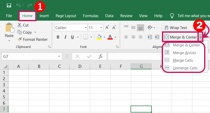
Reason 4# Check For Merged Cells
Another reason for your Excel filter not working is because of the merged cells.
So unmerge if you have any merged cells in the spreadsheet.
If the column headings are being merged, then the Excel filter becomes unable to choose the items present from the merged columns.
The same thing happens with the merged rows. Excel filter won’t count the merged rows data.

For unmerging the cells:
-
Go to the Home tab and to the Alignment group.
-
Now hit the down arrow present across Merge & Center and choose the Unmerge Cells option.
Reason 5# Check For Errors
Check carefully that your data doesn’t include any errors.
Suppose, if you are filtering the ‘Top 10’, ‘Above Average’ or ‘Below Average’ values within your list then using the Number Filters gets compulsory. Otherwise, the error may hinder your Excel application to apply the filter.
- For removing up the errors use the filters to fetch them. Usually, they get listed at the list’s bottom so scroll down.
- Choose the error and tap to the OK option. After locating up the error, fix or delete it and then only clear up the filter.

Reason 6# Check For The Hidden Rows
On the Excel filter, list hidden rows won’t appear as the filter option.
- For unhiding the rows firstly you need to choose the area having the hidden rows. This means you have to choose the rows to present below or above of the hidden data.
- After that either you can make a right-click over the rows header area. Or you can choose the Unhide option. OR just go to the Home tab > cells group> Format> Hide & Unhide> Unhide Rows option.

Reason 7# Check For The Other Filters
Check that your filter is not been left on any other column.
The best option for clearing up all the Excel filters is by tapping to the Clear button present on the ribbon (which is on the right section of the filter button).

This will leave the filter turned on, but it will clear all the filter settings. So now you can make a fresh start with your complete data.
Reason 8# The Filter Button Is Greyed Out
If your Filter function button is appearing gray in color then it means that the filter not working in Excel. The reason behind this can be that your grouped worksheets.
So check out whether your worksheets are grouped or not.
- You can easily identify it by watching out the title bar where generally the filename appears at the screen top.
- If the ‘Your file name’ – Group is appearing then it means that your worksheet is grouped.

- In this case, ungrouping the worksheet can fix filter function not working in Excel issue.
- So come down to your worksheet and make a right-click on the sheet tab. After that choose the Ungroup Sheets option.

- You will see, after making these changes again the filter option starts appearing.
Reason 9# The ‘Equals’ Filter Isn’t Working
While using the Equals filter, Number Filter, or Date Filter, if your Excel is not showing the right data then check whether the format of your data is the same or not.
Suppose, if you are having 2 cells and in each cell, you have entered 1000 as data. One cell is formatted in “currency” format and another one is formatted in “number” format. So when you make use of the “Number Filters, Equals” option, then Excel will only fetch the matches in which you have typed the number format also.
Only typing the text 1000 will search the match for the cells only in the number format. Whereas typing the text $1,000.00 will look for the cells which are formatted as ‘Currency’.
The same rule is also applicable in the case of dates. 16-Jan-19 and 16/01/2019 both are different. Thus make sure that the complete data column is formatted in the same format to avoid filter function not working in Excel issue.
Wrap Up:
The very first thing that Excel filters always check is whether your data matches well with its basic layout standards or not. If you are following all the Excel filters rules then you won’t get Excel filter not working issue.
So, take a close check whether you are following all the above mentioned Excel Filter rules correctly or not.
If none of the above fixes works to resolve your Excel Filter Not Working issue then ask about your queries on our Facebook and Twitter page.


Priyanka is an entrepreneur & content marketing expert. She writes tech blogs and has expertise in MS Office, Excel, and other tech subjects. Her distinctive art of presenting tech information in the easy-to-understand language is very impressive. When not writing, she loves unplanned travels.
Selecting the whole column when applying the filter seems to work
by Matthew Adams
Matthew is a freelancer who has produced a variety of articles on various topics related to technology. His main focus is the Windows OS and all the things… read more
Updated on January 19, 2023
Reviewed by
Vlad Turiceanu

Passionate about technology, Windows, and everything that has a power button, he spent most of his time developing new skills and learning more about the tech world. Coming… read more
- Some users have reported that their Excel filter is not working properly.
- We will show you how to fix the filter in Excel using various methods.
- Depending on your issue, a different solution will work, so be sure to try them accordingly.

Most Excel users probably set up data tables within that application. Users can filter data in their tables with Excel’s filtering tool. However, sometimes Excel spreadsheet tables might not filter the data correctly.
If you need to fix Excel’s table filtering, check out some of the potential resolutions below.
How can I fix Excel table filtering?
1. Select the whole column to apply the filter to
If Excel is not filtering the whole column in a spreadsheet, you can manually configure it to do this. What you need to do is select the column and tweak its filter settings.
1. Launch Microsoft Excel.
2. Open the file where the filter is not working.
3. Select the table’s whole spreadsheet column by clicking the column’s letter.
4. Navigate to the Data tab.
5. Then click the Filter button to apply the filter to the whole column.
6. Click the cell filter arrow button to open the filtering options shown directly below.
7. Uncheck the Blanks checkbox. This setting will ensure that blank cells will not be filtered.
8. Click on OK to apply the changes.
2. Delete blank cells from the table’s column
Alternatively, you can erase blank rows from a table’s column to include values below the empty cells within the filter.
Select all the empty cells’ rows by holding the Ctrl key. Then right-click and select the Delete option.

3. Ungroup sheets
The Filter option will be greyed out when your sheets are grouped together. Thus, you can’t filter spreadsheet tables in grouped sheets. To fix that, right-click the grouped sheets at the bottom of Excel and select Ungroup sheets.

4. Unprotect the worksheet
- Select Excel’s Review tab.
- Press the Unprotect sheet button.

- If an Unprotect sheet window opens, enter the password for the worksheet in the text box.
- Click the OK button.

5. Unmerge cells
- Press the Ctrl + F hotkey.

- Click the Format button on the Find and Replace window.
- Click Merge cells on the Alignment tab shown directly below.

- Press the OK button.
- Press the Find All button.
- Thereafter, the Find and Replace window will list all cell references with merged cells.
- To unmerge merged cells, select a merged cell.
- Click the Merge & Center option on the Home tab.
- Select the Unmerge cells option.


6. Set up a new filter
- If there are rows in your table that don’t get filtered, try setting up a new filter. To do so, select the Data tab.
- Click the Clear button within the Sort & Filter group.
- Then select the table’s full column range with the cursor.
- Click the Filter button on Excel’s Data tab.

Those are some of the resolutions that might get your Excel table filters fixed. In most cases, reapplying filters or clearing them to set up new filters will often resolve Excel filtering issues.
Which of the solutions solved the pro-Excel filtering issue for you? Let us know by leaving a message in the comments section below.
RELATED ARTICLES TO CHECK OUT:
- How to fix Excel’s sharing violation error
- How to fix Microsoft Excel’s File not loaded completely error
- Microsoft Excel cannot add new cells? Check out these tips
Still having issues? Fix them with this tool:
SPONSORED
If the advices above haven’t solved your issue, your PC may experience deeper Windows problems. We recommend downloading this PC Repair tool (rated Great on TrustPilot.com) to easily address them. After installation, simply click the Start Scan button and then press on Repair All.
![]()
Newsletter
| Введение | |
| Excel не фильтрует столбец |
Из этой статьи Вы узнаете как фильтровать столбцы в Excel.
Проблема
Вы хотите отфильтровать столбец, но не видите вообще никаких данных

Фото: AndreyOlegovich.ru
Возможно, эта ошибка вызвана тем, что Вы выделили всею верхнюю сроку под фильтр.
Где-то есть ошибка и она не позволяет фильтровать
Проверьте стоят ли фильтры на всех столбцах, как на картинке ниже или только на одном.

Фото: AndreyOlegovich.ru
Заново выделите верхнюю строку → Нажмите Sort & Filter → Filter

Фото: AndreyOlegovich.ru
Увеличил картинку на случай, если плохо видно

Фото: AndreyOlegovich.ru
Убеждаемся в том, что выделение снятно

Фото: AndreyOlegovich.ru
Выделяем нужный столбец и ставим фильтр снова через Sort & Filter → Filter

Фото: AndreyOlegovich.ru
Убеждаемся в том, что фильтр работает.
Фото: AndreyOlegovich.ru
| MS Excel | |
| VBA | |
| Чередование цвета в строках | |
| Режим разработчика | |
| Цветной выпадающий список | |
| Сортировка чисел | |
| Всё пропало | |
| Перенос строки внутри ячейки Excel | |
| Excel не фильтрует столбец |
Are you are having a few hassles when filtering?
Is the filter not working properly or as you would like it to?
Here are some reasons why your Excel filter may not be working.
Excel has an expectation that you have prepared your data to meet some basic layout standards before you use filter. Get these right and you will minimize filtering hassles.
Check that you are following these Filtering rules…
Now only blank rows will be displayed.
You can easily identify the rows as the row number will now be coloured blue.
To delete the blank rows just select them and then right-click over the top of one of the row blue numbers. Select Delete to delete the rows.
Turn filtering off and you will see that the rows have now been removed.
2. Check your column headings
Check your data has just one row of column headings.
If you need multiple lines for a heading, just type the first line into a cell and then press Alt + Enter to type on a new line within the cell.
Formatting the cell using Wrap Text also works.
3. Check for merged cells
Another reason why your Excel filter may not be working may be due to merged cells.
Unmerge any merged cells or so that each row and column has it’s own individual content.
If your column headings are merged, when you filter you may not be able to select items from one of the merged columns.
If you have merged rows, filtering will not pick up all of the merged rows.
4. Check for errors
Check your data doesn’t include errors. For example, if you were trying to filter on the ‘Top 10’, ‘Above Average’ or ‘Below Average’ values in your list (use Number Filters to do this), and error may stop Excel from applying the filter.
To remove errors first use Filter to find them. They are always listed at the bottom of the list so scroll right to the bottom.
If you see one (or many) remove the check mark from Select All at the top of the list first and then scroll back to the bottom of the list.
Select the error and click OK. Once you have located the error, fix it or delete it and then clear the filter. No go ahead and use Top 10, Above or Below Average and you’ll be back in business!
5. Check for hidden rows
Hidden rows aren’t even shown as a filter option on the filter list.
To unhide rows first select the area containing the hidden rows. This may mean you need to select the row above and below the hidden data.
Then either right-click in the row header area (over the row numbers) and select Unhide or from the Home tab select Format, Hide & Unhide, Unhide Rows.
Extra checks and info…
Check for other filters
Check that a filter hasn’t been left on another column.
The best way to clear all of the filters is to click the Clear button on the Ribbon (to the right of the Filter button).
This then leaves Filter turned on, but removes all filter settings allowing you to start again with the full set of your data.
The Filter button is greyed out
If the Filter button is greyed out check that you don’t have your worksheets grouped.
You can tell if they are simply by looking at the title bar where the filename is shown at the top of the screen.
If you can see ‘Your file name’ — Group you currently have worksheets that are grouped.
Just make your way down to one of your worksheets, right-click the sheet tab and then select Ungroup Sheets. The Filter button will now be available.
The ‘Equals’ filter isn’t working
If you’re using the Number Filter or Date Filter, Equals filter and Excel isn’t returning the correct data, check the formats on your data are the same.
For example, if you have 2 cells with 1,000 entered into each and one cell is formatted with the Currency format and one with the Number, when you use the Number Filters, Equals option, Excel will only find matches where you type the format for the number as well.
Just typing 1000 will find a match for the cell formatted with a Number format only. Typing $1,000.00 will find the cell formatted as Currency.
This is the same for dates. 16-Jan-19 will not match 16/01/2019. Therefore, make sure the entire column of data is formatted with the same format to avoid this problem.
My file is really slow to refresh
If you are finding that your file is starting to become very slow at responding, i.e. the ‘whirly-wheel’ is displayed for more than a few seconds every time you update your file, check that you only selected the table area before you applied Filter, not entire rows, entire columns or the entire worksheet.
Also, if you have applied Filter to multiple tables within the file you might like to remove Filter from any tables you aren’t working with. This may also help eliminate ‘whirly-wheel’ moments.
I hope one of these tips has seen you back on track again. There are so many reasons why your Excel filter may not be working. However, these are typically the ones I come across the most.
Was this blog helpful? Let us know in the Comments below.
Use AutoFilter or built-in comparison operators like «greater than» and “top 10” in Excel to show the data you want and hide the rest. Once you filter data in a range of cells or table, you can either reapply a filter to get up-to-date results, or clear a filter to redisplay all of the data.
Use filters to temporarily hide some of the data in a table, so you can focus on the data you want to see.

Filter a range of data
-
Select any cell within the range.
-
Select Data > Filter.

-
Select the column header arrow
. -
Select Text Filters or Number Filters, and then select a comparison, like Between.
-
Enter the filter criteria and select OK.

 .
.

Filter data in a table
When you put your data in a table, filter controls are automatically added to the table headers.

-
Select the column header arrow
for the column you want to filter. -
Uncheck (Select All) and select the boxes you want to show.
-
Click OK.
The column header arrow
changes to a Filter icon. Select this icon to change or clear the filter.
 for the column you want to filter.
 Filter icon. Select this icon to change or clear the filter.
Related Topics
Excel Training: Filter data in a table
Guidelines and examples for sorting and filtering data by color
Filter data in a PivotTable
Filter by using advanced criteria
Remove a filter
Filtered data displays only the rows that meet criteria that you specify and hides rows that you do not want displayed. After you filter data, you can copy, find, edit, format, chart, and print the subset of filtered data without rearranging or moving it.
You can also filter by more than one column. Filters are additive, which means that each additional filter is based on the current filter and further reduces the subset of data.
Note: When you use the Find dialog box to search filtered data, only the data that is displayed is searched; data that is not displayed is not searched. To search all the data, clear all filters.
The two types of filters
Using AutoFilter, you can create two types of filters: by a list value or by criteria. Each of these filter types is mutually exclusive for each range of cells or column table. For example, you can filter by a list of numbers, or a criteria, but not by both; you can filter by icon or by a custom filter, but not by both.
Reapplying a filter
To determine if a filter is applied, note the icon in the column heading:
-
A drop-down arrow
means that filtering is enabled but not applied.When you hover over the heading of a column with filtering enabled but not applied, a screen tip displays «(Showing All)».
-
A Filter button
means that a filter is applied.When you hover over the heading of a filtered column, a screen tip displays the filter applied to that column, such as «Equals a red cell color» or «Larger than 150».
When you reapply a filter, different results appear for the following reasons:
-
Data has been added, modified, or deleted to the range of cells or table column.
-
Values returned by a formula have changed and the worksheet has been recalculated.
Do not mix data types
For best results, do not mix data types, such as text and number, or number and date in the same column, because only one type of filter command is available for each column. If there is a mix of data types, the command that is displayed is the data type that occurs the most. For example, if the column contains three values stored as number and four as text, the Text Filters command is displayed .
Filter data in a table
When you put your data in a table, filtering controls are added to the table headers automatically.
-
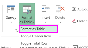
Select the data you want to filter. On the Home tab, click Format as Table, and then pick Format as Table.
-
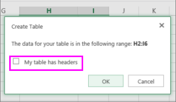
In the Create Table dialog box, you can choose whether your table has headers.
-
Select My table has headers to turn the top row of your data into table headers. The data in this row won’t be filtered.
-
Don’t select the check box if you want Excel for the web to add placeholder headers (that you can rename) above your table data.
-
-
Click OK.
-
To apply a filter, click the arrow in the column header, and pick a filter option.
Filter a range of data
If you don’t want to format your data as a table, you can also apply filters to a range of data.
-
Select the data you want to filter. For best results, the columns should have headings.
-
On the Data tab, choose Filter.
Filtering options for tables or ranges
You can either apply a general Filter option or a custom filter specific to the data type. For example, when filtering numbers, you’ll see Number Filters, for dates you’ll see Date Filters, and for text you’ll see Text Filters. The general filter option lets you select the data you want to see from a list of existing data like this:
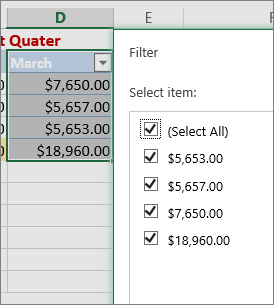
Number Filters lets you apply a custom filter:
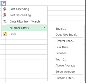
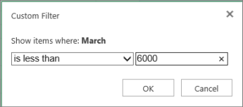
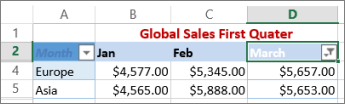
In this example, if you want to see the regions that had sales below $6,000 in March, you can apply a custom filter:
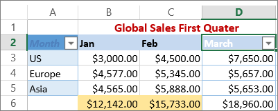
Here’s how:
-
Click the filter arrow next to March > Number Filters > Less Than and enter 6000.
-
Click OK.
Excel for the web applies the filter and shows only the regions with sales below $6000.
You can apply custom Date Filters and Text Filters in a similar manner.
To clear a filter from a column
-
Click the Filter
button next to the column heading, and then click Clear Filter from <«Column Name»>.
To remove all the filters from a table or range
-
Select any cell inside your table or range and, on the Data tab, click the Filter button.
This will remove the filters from all the columns in your table or range and show all your data.
-
Click a cell in the range or table that you want to filter.
-
On the Data tab, click Filter.
-
Click the arrow
in the column that contains the content that you want to filter. -
Under Filter, click Choose One, and then enter your filter criteria.

 in the column that contains the content that you want to filter.
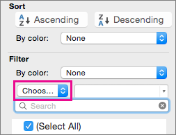
Notes:
-
You can apply filters to only one range of cells on a sheet at a time.
-
When you apply a filter to a column, the only filters available for other columns are the values visible in the currently filtered range.
-
Only the first 10,000 unique entries in a list appear in the filter window.
-
Click a cell in the range or table that you want to filter.
-
On the Data tab, click Filter.
-
Click the arrow
in the column that contains the content that you want to filter. -
Under Filter, click Choose One, and then enter your filter criteria.
-
In the box next to the pop-up menu, enter the number that you want to use.
-
Depending on your choice, you may be offered additional criteria to select:
Notes:
-
You can apply filters to only one range of cells on a sheet at a time.
-
When you apply a filter to a column, the only filters available for other columns are the values visible in the currently filtered range.
-
Only the first 10,000 unique entries in a list appear in the filter window.
-
Instead of filtering, you can use conditional formatting to make the top or bottom numbers stand out clearly in your data.
You can quickly filter data based on visual criteria, such as font color, cell color, or icon sets. And you can filter whether you have formatted cells, applied cell styles, or used conditional formatting.
-
In a range of cells or a table column, click a cell that contains the cell color, font color, or icon that you want to filter by.
-
On the Data tab, click Filter .
-
Click the arrow
in the column that contains the content that you want to filter. -
Under Filter, in the By color pop-up menu, select Cell Color, Font Color, or Cell Icon, and then click a color.
 in the column that contains the content that you want to filter.
This option is available only if the column that you want to filter contains a blank cell.
-
Click a cell in the range or table that you want to filter.
-
On the Data toolbar, click Filter.
-
Click the arrow
in the column that contains the content that you want to filter. -
In the (Select All) area, scroll down and select the (Blanks) check box.
Notes:
-
You can apply filters to only one range of cells on a sheet at a time.
-
When you apply a filter to a column, the only filters available for other columns are the values visible in the currently filtered range.
-
Only the first 10,000 unique entries in a list appear in the filter window.
-
-
Click a cell in the range or table that you want to filter.
-
On the Data tab, click Filter .
-
Click the arrow
in the column that contains the content that you want to filter. -
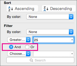
Under Filter, click Choose One, and then in the pop-up menu, do one of the following:
To filter the range for
Click
Rows that contain specific text
Contains or Equals.
Rows that do not contain specific text
Does Not Contain or Does Not Equal.
-
In the box next to the pop-up menu, enter the text that you want to use.
-
Depending on your choice, you may be offered additional criteria to select:
To
Click
Filter the table column or selection so that both criteria must be true
And.
Filter the table column or selection so that either or both criteria can be true
Or.
-
Click a cell in the range or table that you want to filter.
-
On the Data toolbar, click Filter .
-
Click the arrow
in the column that contains the content that you want to filter. -
Under Filter, click Choose One, and then in the pop-up menu, do one of the following:
To filter for
Click
The beginning of a line of text
Begins With.
The end of a line of text
Ends With.
Cells that contain text but do not begin with letters
Does Not Begin With.
Cells that contain text but do not end with letters
Does Not End With.
-
In the box next to the pop-up menu, enter the text that you want to use.
-
Depending on your choice, you may be offered additional criteria to select:
To
Click
Filter the table column or selection so that both criteria must be true
And.
Filter the table column or selection so that either or both criteria can be true
Or.
Wildcard characters can be used to help you build criteria.
-
Click a cell in the range or table that you want to filter.
-
On the Data toolbar, click Filter.
-
Click the arrow
in the column that contains the content that you want to filter. -
Under Filter, click Choose One, and select any option.
-
In the text box, type your criteria and include a wildcard character.
For example, if you wanted your filter to catch both the word «seat» and «seam», type sea?.
-
Do one of the following:
Use
To find
? (question mark)
Any single character
For example, sm?th finds «smith» and «smyth»
* (asterisk)
Any number of characters
For example, *east finds «Northeast» and «Southeast»
~ (tilde)
A question mark or an asterisk
For example, there~? finds «there?»
Do any of the following:
|
To |
Do this |
|---|---|
|
Remove specific filter criteria for a filter |
Click the arrow |
|
Remove all filters that are applied to a range or table |
Select the columns of the range or table that have filters applied, and then on the Data tab, click Filter. |
|
Remove filter arrows from or reapply filter arrows to a range or table |
Select the columns of the range or table that have filters applied, and then on the Data tab, click Filter. |
When you filter data, only the data that meets your criteria appears. The data that doesn’t meet that criteria is hidden. After you filter data, you can copy, find, edit, format, chart, and print the subset of filtered data.
Table with Top 4 Items filter applied
Filters are additive. This means that each additional filter is based on the current filter and further reduces the subset of data. You can make complex filters by filtering on more than one value, more than one format, or more than one criteria. For example, you can filter on all numbers greater than 5 that are also below average. But some filters (top and bottom ten, above and below average) are based on the original range of cells. For example, when you filter the top ten values, you’ll see the top ten values of the whole list, not the top ten values of the subset of the last filter.
In Excel, you can create three kinds of filters: by values, by a format, or by criteria. But each of these filter types is mutually exclusive. For example, you can filter by cell color or by a list of numbers, but not by both. You can filter by icon or by a custom filter, but not by both.
Filters hide extraneous data. In this manner, you can concentrate on just what you want to see. In contrast, when you sort data, the data is rearranged into some order. For more information about sorting, see Sort a list of data.
When you filter, consider the following guidelines:
-
Only the first 10,000 unique entries in a list appear in the filter window.
-
You can filter by more than one column. When you apply a filter to a column, the only filters available for other columns are the values visible in the currently filtered range.
-
You can apply filters to only one range of cells on a sheet at a time.
Note: When you use Find to search filtered data, only the data that is displayed is searched; data that is not displayed is not searched. To search all the data, clear all filters.
Need more help?
You can always ask an expert in the Excel Tech Community or get support in the Answers community.
Excel Column Filter (Table of Contents)
- Filter Column in Excel
- How to Filter a Column in Excel?
Filter Column in Excel
Filters in Excel are used for filtering the data by selecting the data type in the filter dropdown. By using a filter, we can make out the data that we want to see or on which we need to work.
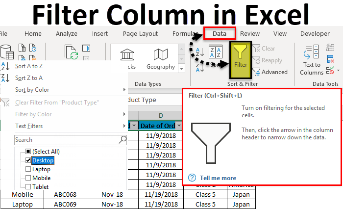
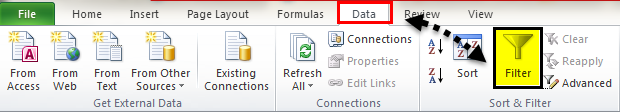
To access/apply a filter in any column of excel, go to the Data menu tab; under Sort & Filter, we will find the Filter option.
How to Filter a Column in Excel?
To filter a column in excel is a very simple and easy task. Let’s understand the working of how to filter a column in Excel with an example.
You can download this Column Filter Excel Template here – Column Filter Excel Template
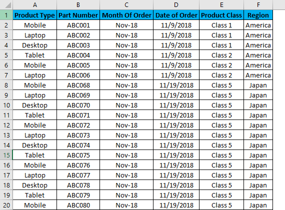
We have some sample data tables in excel, where we will apply the filter in columns. Below is the screenshot of a data set, which has multiple columns and multiple rows with various data sets.
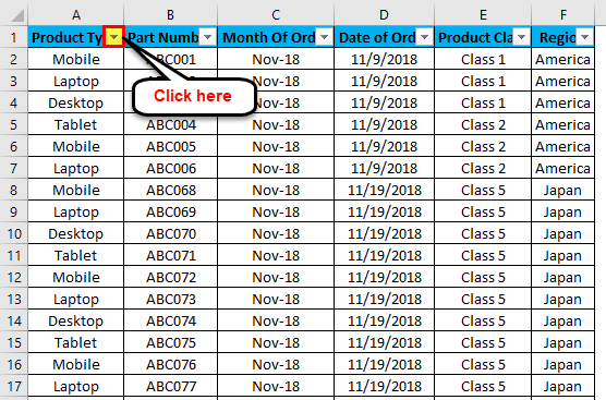
For applying Excel Column Filter, select the top row first, and the filter will be applied to the selected row only, as shown below. Sometimes when we work for a large set of data and select the filter directly, the current look of the sheet can be applied.
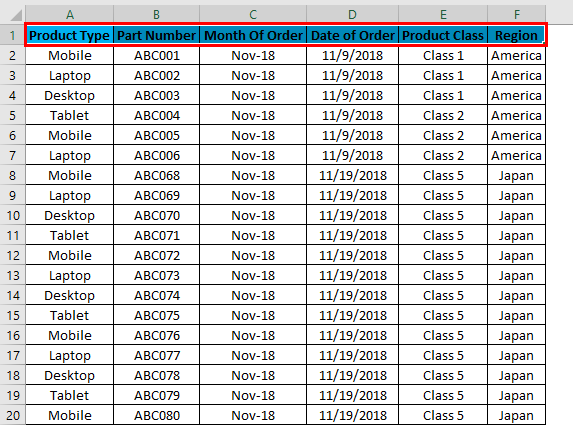
As we can see in the above screenshot, row 1 is selected, and it is ready to apply the filters.
Now for applying filters, go to the Data menu, and under Sort & Filters, select Filters.
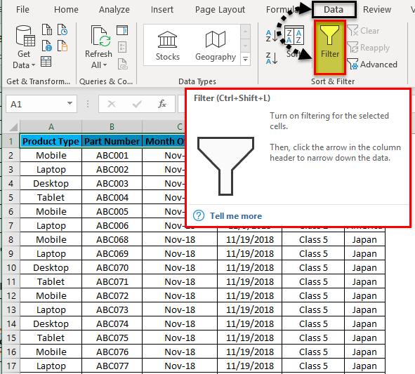
Once we click on Filters, we can see the filters will be applied in the selected row, as shown in the below screenshot.
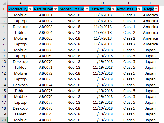
The top row 1 now has the dropdown. This drop-down is those things by which we can filter the data as per our need.
To open the drop-down option in an applied filter, click on the down arrow (as shown below) or go to any column top and press Alt + Down.
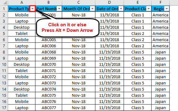
A drop-down menu will appear, as shown in the below screenshot.
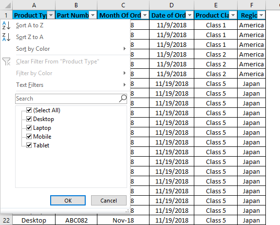
As we can see in the above screenshot, there are few filter options provided by Microsoft.
- Sort A to Z / Sort Oldest to Newest (for dates) / Sort Smallest to Largest (for numbers)
- Sort Z to A / Sort Newest to Oldest (for dates) / Sort Largest to Smallest (for numbers)
- Sort by Color
- Clear Filter From “Product Type” (This would entitle the name of columns where a filter is applied)
- Filter by Color
- Text Filters
- Search/Manual Filter
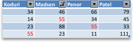
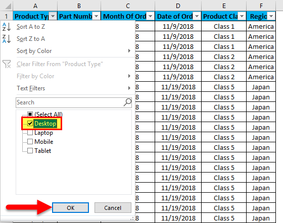
As we can see in the first screenshot, where data is in a randomly scattered format. Let us apply the filter and see what changes happen in the data. For that, go to column A and in the drop-down menu, select only Desktops, as shown in the below screenshot, and click on OK.
Once we do it, we will see, the data is now filtered with Desktop. And whatever the data is there in w.r.t. Desktop in the rest of the columns will also get filtered, as the screenshot below.
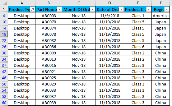
As we can see in the above screenshot, data is now filtered with Desktop, and all the columns are also sorted with data available for Desktop. Also, the line numbers, which are circled in the above screenshot, are also showing the random numbers. This means that the filter which we have applied was in a random format, so the line numbers have also been scattered when we applied the filter.
Now, let’s try to apply the text filter, which is a very interesting part of filtering the data. For that, go to any of the columns, and click on the drop-down button to see the filter options.
Now go to Text Filters.
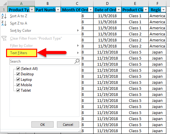
We will find a few more options available for filtering the data, as shown in the below screenshot.
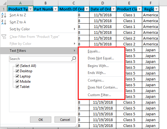
The highlighted portion of Text Filters in the box has Equals, Does Not Equal, Begins With, Ends With, Contains, Does Not Contain, and Custom Filter.
- Equal: With this, we can filter the data with an exact equal word available in the data.
- Does Not Equal: With this, we can filter the data with a word that does not match the available words in the data.
- Begins With: This filters the data, which begins with a specific word or letter, or character.
- Ends With – This filters the data, which ends with a specific word or letter, or character.
- Contains: With this, we can filter the data which contains any specific word or letter, or character.
- Does Not Contain: With this, we can filter the data which does not contain any specific word, letter, or character.
- Custom Filter: With this, we can apply any combination of the above-mentioned Text Filters in data together to get data filtered more deeply and specific to our requirement. Once we click on Custom Filter, we will get a box of Custom AutoFilter, as shown in the below screenshot.
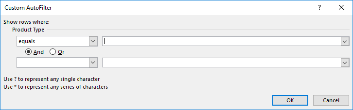
As we can see in the above screenshot of Custom AutoFilter, it has to two filter options at the left sides, which And and Or check-in circles separate. And the other two boxes provided on the left side are for filling the criteria values. This can be called a smart filter.
There are different ways of applying the Excel column filter.
- Data menu -> Filter
- By pressing Ctrl + Shift + L together.
- By pressing Alt + D + F + F simultaneously.
Pros of Excel Column Filter
- By applying filters, we can sort the data as per our needs.
- By filters, performing the analysis or any work becomes easy.
- Filters sort the data with words, numbers, cell colors, font colors, or with any range. Also, multiple criteria can be used as well.
Cons of Excel Column Filter
- Filters can be applied to all kinds of range sizes, but it is not useful if the data size increases up to a certain limit. For some cases, if the data is going beyond 50,000 lines, then it becomes slow, and sometimes it does not show data available in any column.
Things to Remember
- If you are using filter and freeze panel together, then first apply the filter and then use freeze panel. By doing this, data will be frozen from the middle portion of the sheet.
- Avoid or be cautious while using a filter for huge sets of data (maybe for 50000 or more). It will take a lot more time to get applied, and sometimes the file also gets crashed.
Recommended Articles
This has been a guide to Filter Column in Excel. Here we discuss how to filter a column in Excel along with practical examples and a downloadable excel template. You can also go through our other suggested articles –
- Excel AutoFilter
- Excel Data Filter
- Advanced Filter in Excel
- VBA Filter
If you’re dealing with a rather large database, then the filter function on Excel can come in handy. This function allows you to sort the dataset according to your set conditions. As a result, it makes analyzing and summarising data much easier.
However, there might be instances where the filter function might not be working properly. Usually, such an error pops up when there are blank cells within the dataset. So, a quick fix to the issue is to delete these cells.
But, what if the issue persists? In this article, let’s learn more about the potential causes and the fixes for the filter function not working on Excel.
Why is My Excel Filter Not Working?
Here is a list of the potential causes of why the filter function might not be working in your Excel application.
- Blank or Hidden Rows between the dataset
- Vertical Merged Cells
- Data Value Error
- Selected more than one worksheet (grouped)
- The worksheet is protected
How to Fix Excel Filter Not Working?
Now that we know have listed out the causes, let’s jump right in with applying the troubleshooting methods for this issue.
Select All Data From Sheet
If your dataset has blank rows or columns, it might not select the area (row or column) below or past these cells. As a result, Excel will fail to filter out all the data in your dataset.
To be on the safe end, we suggest that you manually select the data. Now, click on the Filter ribbon and choose how you would like to arrange it. This method should be able to include all the datasets.
Remove Blank Rows/Columns
Alternatively, you can also remove the blank rows by configuring the data on your Filter area. Here is how you can do so.
- Head over to the column that showcases the filter list.
- Click on the drop-down arrow and uncheck the box for Select All.
- Scroll further down, and check the option for Blanks.
- Hit the OK button to save filter changes.


You can also manually delete these cells. To do so, right-click on the row adjacent to the blank cell. Select the Delete option to remove these blank rows/columns.
Unhide Rows or Columns
If you have hidden rows or columns on your dataset, then Excel won’t apply the Filter function on these data cells. You will have to unhide any hidden rows or columns from your sheet.
Here is how you can do it.
- Spot the hidden row/column.
- It should represent a double line inside the row headings. Skipped order of number or alphabets is another sign of how to recognize hidden rows/columns.
- Select both the adjacent row/columns.
- Navigate to the Home tab and click on Format.
- From the drop-down menu, select Hide & Unhide.
- Finally, click on Unhide Rows or Unhide Columns.


Unmerge Cells
Merged cells in your dataset can also create problems while you’re trying to filter your table. Excel tends to disregard the data on merged rows/columns. So, we suggest that you first unmerge all data cells before using the filter option.
Here is a step-by-step guide on how you can do it.
- Click on the Merged Cell on your sheet.
- Under the Home tab, navigate to the Alignment section.
- Click on Merge and Center, and from the drop-down menu, select the Unmerge cells option.


Remove Data Errors
If there are data errors in your table, then the filter function might not work on your data set. So, It is best to remove these data errors from the table.
Here is a step-by-step guide on how you can do it.
- Head over to the column that showcases the filter list.
- Click on the drop-down arrow and uncheck the box for Select All.
- Scroll further down, and check the option for #Value!
- Hit the OK button to save filter changes.
Clear and Add Filter
In some rare cases, the current filter you’re setting up might not work on your data set. So, a quick troubleshooting method you can apply is to clear the previous filter and set up a new one.
Here is how you can do it.
- Head over to the Data menu.
- Click on the Clear icon right next to the Filter button.

- Select the column heading or the dataset.
- Now, click on the Filter button.

How to Fix Filter Grayed Out in Excel?
Here are a few effective methods you can apply when the filter option is grayed out on your Excel Application.
Ungroup Sheets
If you have selected more than one sheet, then Excel will not give you access to the Filter function. First and foremost, you will have to ungroup the sheets. To do so, right-click on a sheet from the bottom bar, and click on the Ungroup Sheets option.
Unprotect the Sheet
Another factor you should look out for is to check whether your sheet is protected or not. When you’re sheet is protected, Excel automatically greys out the Filter option. So, to unprotect the sheet,
- Open up the Excel document.
- Head over to the Review tab on Excel.
- Click on the Unprotect Sheet option.

- Now, a pop window will appear, type in your password for the sheet.
- Finally, click on the OK button to confirm your action.

Related Questions
Why is my Filter by color not Working?
If your filtering by color is not working on your spreadsheet, then there are two reasons why it might occur. The first is if there is only one specific color in all your cells or if you have shared the workbook. To unshare, head over to Review > Unshare Workbook.
How to fix Excel Not Grouping Dates in Filters?
In some instances, the grouping dates in filters might get disabled. So, here is a step-by-step guide on how you can enable it.
- Head over to the File menu.
- Select Options.

- From the left panel, head over to the Advanced tab.
- Under the Display Option for this Workbook section, check the option for Group Dates in the AutoFilter menu.


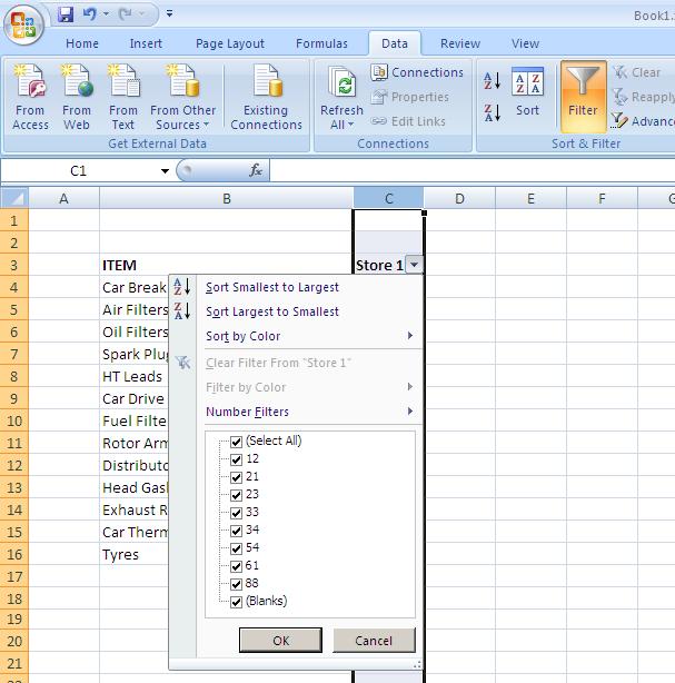
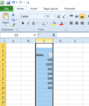
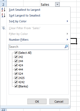
One of the most common problem with filter function is that it stops working beyond a blank row. Filter will not include cells beyond the first blank.
To avoid this issue, select the range before applying the filter function. Please refer to the following excel spreadsheet for example.
1. Before applying filter on column C, either select the entire column C or the data that needs to be filtered.
![]()
2. Select Filter option under Data tab. Now all items appear in the filtered list as well as filter checkbox list.
![]()
Similarly you may select multiple columns or a range of cells before applying the filter.
![]()
External links for other issues that might prevent filter function to work properly.
Reasons why your Excel filter may not be working
Excel how to filter properly
Filters do not include cells beyond first blank
Search engine keywords for this question:
Filter function not working properly in Excel 2007, 2010
Excel not filtering the entire column
Excel not filtering all entries
Filter not showing all data in a column
Unable to filter properly in MS Excel