
Excel for Microsoft 365 for Mac Excel 2021 for Mac Excel 2019 for Mac Excel 2016 for Mac Excel for Mac 2011 More…Less
Cause: The default cell reference style (A1), which refers to columns as letters and refers to rows as numbers, was changed.
Solution: Clear the R1C1 reference style selection in Excel preferences.
Difference between A1 and R1C1 reference styles
-
On the Excel menu, click Preferences.
-
Under Authoring, click Calculation
 .
. -
Clear the Use R1C1 reference style check box.
The column headings now show A, B, and C, instead of 1, 2, 3, and so on.
 .
.Need more help?

This Excel tutorial explains how to change column headings from numbers (1, 2, 3, 4) back to letters (A, B, C, D) in Excel 2016 (with screenshots and step-by-step instructions).
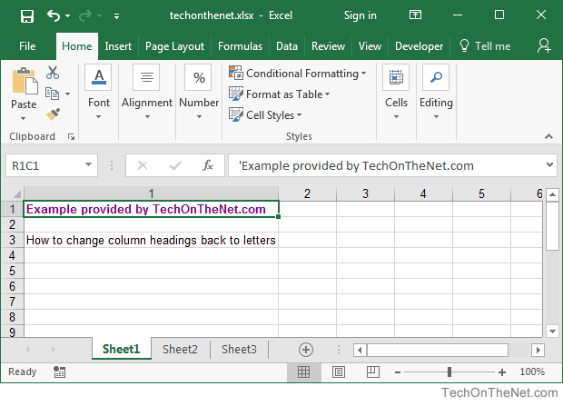
Question: In Microsoft Excel 2016, my Excel spreadsheet has numbers for both rows and columns. How do I change the column headings back to letters such as A, B, C, D?
Answer: Traditionally, column headings are represented by letters such as A, B, C, D. If your spreadsheet shows the columns as numbers, you can change the headings back to letters with a few easy steps.
In the example below, the column headings are numbered 1, 2, 3, 4 instead of the traditional A, B, C, D values that you normally see in Excel. When the column headings are numeric values, R1C1 reference style is being displayed in the spreadsheet.
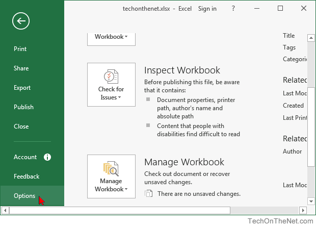
To change the column headings to letters, select the File tab in the toolbar at the top of the screen and then click on Options at the bottom of the menu.
When the Excel Options window appears, click on the Formulas option on the left. Then uncheck the option called «R1C1 reference style» and click on the OK button.

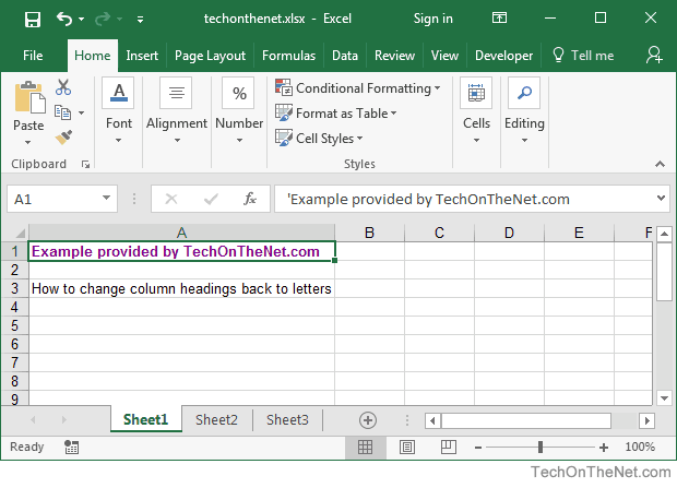
Now when you return to your spreadsheet, the column headings should be letters (A, B, C, D) instead of numbers (1, 2, 3, 4).
Содержание
- Columns and rows are labeled numerically in Excel
- Symptoms
- Cause
- Resolution
- More information
- A1 Reference Style vs. R1C1 Reference Style
- The A1 Reference Style
- The R1C1 Reference Style
- References
- How to Show Column Letters Instead of Numbers in Excel
- Effect of numbers instead of letters in column headings
- Steps for changing from column letters to numbers
- How to number columns in Excel and convert column letter to number
- How to return column number in Excel
- How to convert column letter to number (non-volatile formula)
- Change column letter to number using a custom function
- Return column number of a specific cell
- Get column letter of the current cell
- How to show column numbers in Excel
- How to number columns in Excel
- Converting column letter to number [duplicate]
- 5 Answers 5
- MS Excel 2016: How to Change Column Headings from Numbers to Letters
Columns and rows are labeled numerically in Excel
Symptoms
Your column labels are numeric rather than alphabetic. For example, instead of seeing A, B, and C at the top of your worksheet columns, you see 1, 2, 3, and so on.
Cause
This behavior occurs when the R1C1 reference style check box is selected in the Options dialog box.
Resolution
To change this behavior, follow these steps:
- Start Microsoft Excel.
- On the Tools menu, click Options.
- Click the Formulas tab.
- Under Working with formulas, click to clear the R1C1 reference style check box (upper-left corner), and then click OK.
If you select the R1C1 reference style check box, Excel changes the reference style of both row and column headings, and cell references from the A1 style to the R1C1 style.
More information
A1 Reference Style vs. R1C1 Reference Style
The A1 Reference Style
By default, Excel uses the A1 reference style, which refers to columns as letters (A through IV, for a total of 256 columns), and refers to rows as numbers (1 through 65,536). These letters and numbers are called row and column headings. To refer to a cell, type the column letter followed by the row number. For example, D50 refers to the cell at the intersection of column D and row 50. To refer to a range of cells, type the reference for the cell that is in the upper-left corner of the range, type a colon (:), and then type the reference to the cell that is in the lower-right corner of the range.
The R1C1 Reference Style
Excel can also use the R1C1 reference style, in which both the rows and the columns on the worksheet are numbered. The R1C1 reference style is useful if you want to compute row and column positions in macros. In the R1C1 style, Excel indicates the location of a cell with an «R» followed by a row number and a «C» followed by a column number.
References
For more information about this topic, click Microsoft Excel Help on the Help menu, type about cell and range references in the Office Assistant or the Answer Wizard, and then click Search to view the topic.
Источник
How to Show Column Letters Instead of Numbers in Excel
Excel has an option for showing column letters instead of number. This can be useful, for example, when you work with VBA macros or when you have to count columns (e.g. VLOOKUP). But in most cases, you would prefer letters. In this article we learn how to change column numbers to letters and the other way around in Excel.
Effect of numbers instead of letters in column headings
If you see numbers instead of letters for the column headings, you will also notice the following effect: All cell references are replaced by numbers. This style is called R1C1 reference style.
Instead of ‘=$A$2’, you will find ‘=R1C2’ for r ow 1 and c olumn 2. If we remove the dollar signs, this formula might look completely different as it will always show the distance from the current cell.
Steps for changing from column letters to numbers
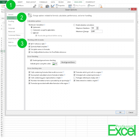
You can switch from column letters to numbers quite easily in Excel (the following numbers are referring to the picture above):
- Go To File and click on Options.
- Select Formulas on the left hand side.
- Tick “R1C1 reference style”.
Switching back from numbers to letters works the same way. Only in the last step, you have to remove the tick from “R1C1 reference style”.
Please note that all references within formulas will be replaced by numbers.
Henrik Schiffner is a freelance business consultant and software developer. He lives and works in Hamburg, Germany. Besides being an Excel enthusiast he loves photography and sports.
Источник
How to number columns in Excel and convert column letter to number
 by Svetlana Cheusheva, updated on March 9, 2023
The tutorial talks about how to return a column number in Excel using formulas and how to number columns automatically.
Last week, we discussed the most effective formulas to change column number to alphabet. If you have an opposite task to perform, below are the best techniques to convert a column name to number.
How to return column number in Excel
To convert a column letter to column number in Excel, you can use this generic formula:
For example, to get the number of column F, the formula is:
And here’s how you can identify column numbers by letters input in predefined cells (A2 through A7 in our case):
Enter the above formula in B2, drag it down to the other cells in the column, and you will get this result: 
How this formula works:
First, you construct a text string representing a cell reference. For this, you concatenate a letter and number 1. Then, you hand off the string to the INDIRECT function to convert it into an actual Excel reference. Finally, you pass the reference to the COLUMN function to get the column number.
How to convert column letter to number (non-volatile formula)
Being a volatile function, INDIRECT can significantly slow down your Excel if used broadly in a workbook. To avoid this, you can identify the column number using a slightly more complex non-volatile alternative:
This works perfectly in dynamic array Excel (365 and 2021). In older version, you need to enter it as an array formula (Ctrl + Shift + Enter) to get it to work.
=MATCH(A2&»1″, ADDRESS(1, COLUMN($1:$1), 4), 0)
Or you can use this non-array formula in all Excel versions:
=MATCH(A2&»1″, INDEX(ADDRESS(1, INDEX(COLUMN($1:$1), ), 4), ), 0) 
How this formula works:
First off, you concatenate the letter in A2 and the row number «1» to construct a standard «A1» style reference. In this example, we have letter «A» in A2, so the resulting string is «A1».
Next, you get an array of strings representing all cell addresses in the first row, from «A1» to «XFD1». For this, you use the COLUMN($1:$1) function, which generates a sequence of column numbers, and pass that array to the column_num argument of the ADDRESS function:
Given that row_num (1st argument) is set to 1 and abs_num (3rd argument) is set to 4 (meaning you want a relative reference), the ADDRESS function delivers this array:
Finally, you build a MATCH formula that searches for the concatenated string in the above array and returns the position of the found value, which corresponds to the column number you are looking for:
Change column letter to number using a custom function
«Simplicity is the ultimate sophistication,» stated the great artist and scientist Leonardo da Vinci. To get a column number from a letter in an easy way, you can create your own custom function.
Fully in line with the above principle, the function’s code is as simple as it can possibly be:
Insert the code in your VBA editor as explained here, and your new function named ColumnNumber is ready for use.
The function requires just one argument, col_letter, which is the column letter to be converted into a number:
Your real formula can be as follows:
If you compare the results returned by our custom function and Excel’s native ones, you will make sure they are exactly the same: 
Return column number of a specific cell
To get a column number of a particular cell, simply use the COLUMN function:
For instance, to identify the column number of cell B3, the formula is:
Obviously, the result is 2. 
Get column letter of the current cell
To find out a column number of the current cell, use the COLUMN() function with an empty argument, so it refers to the cell where the formula is:
=COLUMN() 
How to show column numbers in Excel
By default, Excel uses the A1 reference style and labels column headings with letters and rows with numbers. To get columns labeled with numbers, change the default reference style from A1 to R1C1. Here’s how:
- In your Excel, click File >Options.
- In the Excel Options dialog box, select Formulas in the left pane.
- Under Working with formulas, check the R1C1 reference style box, and click OK.
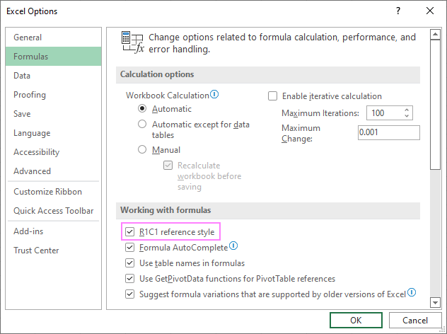
The column labels will immediately change from letters to numbers: 
Please note that selecting this option will not only change column labels — cell addresses will also change from A1 to R1C1 references, where R means «row» and C means «column». For example, R1C1 refers to the cell in row 1 column 1, which corresponds to the A1 reference. R2C3 refers to the cell in row 2 column 3, which corresponds to the C2 reference.
In existing formulas, cell references will update automatically, while in new formulas you will have to use the R1C1 reference style.
Tip. To revert back to A1 style, uncheck the R1C1 reference style check box in Excel Options.
How to number columns in Excel
If you are not used to the R1C1 reference style and want to keep A1 references in your formulas, then you can insert numbers in the first row of our worksheet, so you have both — column letters and numbers. This can be easily done with the help of the Auto Fill feature.
Here are the detailed steps:
- In A1, type number 1.
- In B1, type number 2.
- Select cells A1 and B1.
- Hover the cursor over a small square in the lower right corner of cell B1, which is called the Fill handle. As you do this, the cursor will change to a thick black cross.
- Drag the fill handle to the right up to the column you need.

As a result, you will retain the column labels as letters, and underneath the letters you will have the column numbers.
Tip. To keep the columns numbers in view while scrolling to the below areas of the worksheet, you can freeze top row.
That’s how to return column numbers in Excel. I thank you for reading and look forward to seeing you on our blog next week!
Источник
Converting column letter to number [duplicate]
I found code to convert number to column letter.
How can I convert from column letter to number?
5 Answers 5
You can reference columns by their letter like this:
So to get the column number, just modify the above code like this:
The above line returns an integer (1 in this case).
So if you were using the variable mycolumn to store and reference column numbers, you could set the value this way:
And then you could reference your variable this way:
or to reference a cell ( A1 ):
or to reference a range of cells ( A1:A10 )you could use:
The answer given may be simple but it is massively sub-optimal, because it requires getting a Range and querying a property. An optimal solution would be as follows:

To see the numerical equivalent of a letter-designated column:

My Comments
ARich gives a good solution and shows the method I used for a while but Sancarn is right, its not optimal. It’s a little slower, will cause errors if the wrong input is given, and is not very robust. Sancarn is on the right track, but lacks a little error checking: for example, getColIndex(«_») and getColIndex(«AE»), will both return 31. Other non-letter characters (ex: «*») sometimes return various negative values.
Working Function
Here is a function I wrote that will convert a column letter into a number. If the input is not a column on the worksheet, it will return -1 (unless AllowOverflow is set to TRUE).
Источник
MS Excel 2016: How to Change Column Headings from Numbers to Letters
This Excel tutorial explains how to change column headings from numbers (1, 2, 3, 4) back to letters (A, B, C, D) in Excel 2016 (with screenshots and step-by-step instructions).
See solution in other versions of Excel :
Question: In Microsoft Excel 2016, my Excel spreadsheet has numbers for both rows and columns. How do I change the column headings back to letters such as A, B, C, D?
Answer: Traditionally, column headings are represented by letters such as A, B, C, D. If your spreadsheet shows the columns as numbers, you can change the headings back to letters with a few easy steps.
In the example below, the column headings are numbered 1, 2, 3, 4 instead of the traditional A, B, C, D values that you normally see in Excel. When the column headings are numeric values, R1C1 reference style is being displayed in the spreadsheet.
To change the column headings to letters, select the File tab in the toolbar at the top of the screen and then click on Options at the bottom of the menu.
When the Excel Options window appears, click on the Formulas option on the left. Then uncheck the option called «R1C1 reference style» and click on the OK button.
Now when you return to your spreadsheet, the column headings should be letters (A, B, C, D) instead of numbers (1, 2, 3, 4).
Источник
Skip to content
![]()
Excel has an option for showing column letters instead of number. This can be useful, for example, when you work with VBA macros or when you have to count columns (e.g. VLOOKUP). But in most cases, you would prefer letters. In this article we learn how to change column numbers to letters and the other way around in Excel.
Effect of numbers instead of letters in column headings
If you see numbers instead of letters for the column headings, you will also notice the following effect: All cell references are replaced by numbers. This style is called R1C1 reference style.
Instead of ‘=$A$2’, you will find ‘=R1C2’ for row 1 and column 2. If we remove the dollar signs, this formula might look completely different as it will always show the distance from the current cell.
Steps for changing from column letters to numbers
You can switch from column letters to numbers quite easily in Excel (the following numbers are referring to the picture above):
- Go To File and click on Options.
- Select Formulas on the left hand side.
- Tick “R1C1 reference style”.
Switching back from numbers to letters works the same way. Only in the last step, you have to remove the tick from “R1C1 reference style”.
Please note that all references within formulas will be replaced by numbers.

Henrik Schiffner is a freelance business consultant and software developer. He lives and works in Hamburg, Germany. Besides being an Excel enthusiast he loves photography and sports.
We use cookies on our website to give you the most relevant experience by remembering your preferences and repeat visits. By clicking “Accept”, you consent to the use of ALL the cookies.
.
Earlier, we learnt how to convert the column number to the letter. But how do we convert column letter to number in excel? In this article, we learn to convert excel column to number.

So we have a function named COLUMN that returns the column number of supplied reference. We will use the COLUMN function with INDIRECT function to get the column number from a given column letter.
Generic Formula to convert letters to numbers in excel
Col_letter: it is the reference of the column letter of which you want to get column number.
Var2:
Let’s see an example to make things clear.
Example: Create an excel column letter to number converter
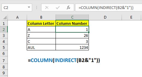
Here we have some column letters in B2:B5. We want to get corresponding column number (1, 2, 3, etc.) from that given letter (A, B, C, etc.).
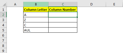
Apply the above generic formula here to get column number of a given letter.
Copy it down. You will have the column number of the given column letter in B2:B5.
How does it work?
Well, it is very simple. The idea is to get the first cell’s reference from the given column number. And then use COLUMN function to get the column number of a given column letter.
Here, INDIRECT(B2&»1″) translates to INDIRECT(“A1″). This then gives us the cell reference of A1.
Eventually, we get COLUMN(A1), which then returns the column number of a given column letter.
So yeah, this is how to convert a column letter into a column index number. This is quite easy. Let me know if you have any doubt regarding this function or any other function in advanced excel. The comments section is all yours.
Download file:
Related Articles:
How to Convert Excel Column Number To Letter
Popular Articles:
The VLOOKUP Function in Excel
COUNTIF in Excel 2016
How to Use SUMIF Function in Excel
Have you ever opened an Excel workbook and found that the column headings show numbers instead of letters? The formula look strange too, showing references like RC[-1] instead of D2.

This is R1C1 reference style — a handy feature, and I use it sometimes when programming or setting up a workbook.
Numbers on the column headings make it easier to set up formulas that need a column number, such as VLOOKUP. I don’t have to get fingerprints on my screen, as I count across to column R, where the lookup value is.
Video: Change Excel Column Headings from Numbers to Letters
To see why this happens, and how to switch the column headings back to letters, watch this short video tutorial. The written instructions are below the video.
Your browser can’t show this frame. Here is a link to the page
Why It Happens
Maybe you’ve never heard of R1C1 reference style, and certainly didn’t change any settings. If you didn’t turn that option on, why did the numbers suddenly appear? Probably because someone sent you a workbook, and that’s the first Excel file that you opened today.
The first workbook that you open, when opening Excel, sets the reference style. For example, perhaps I built a workbook for you, and saved it while I was using R1C1 reference style.
I sent you the workbook overnight, and it was the first thing you opened this morning. Surprise! There are numbers in the column headings.
Turn R1C1 Reference Style On or Off
If you close Excel, then open a workbook that you created yourself, with letters in the column headings, that will change the reference style back to A1, which has letters in the column headings.
Or, to manually change the reference style, you can change the option setting.
In Excel 2010:
- At the left end of the Ribbon, click the File tab, then click Options.
- Click the Formulas category.
- In the Working with Formulas section, add or remove the check mark from ‘R1C1 reference style’
- Click OK to close the Options window.

In Excel 2007:
-
- At the left end of the Ribbon, click the Office Button, then click Excel Options.
- Click the Formulas category.
- In the Working with Formulas section, add or remove the check mark from ‘R1C1 reference style’
- Click OK to close the Options window.
In Excel 2003 and earlier versions:
- On the Tools menu, click Options and select the General tab.
- Add or remove the check mark from ‘R1C1 reference style’
- Click OK to close the Options dialog box.

Use a Macro to Switch Headings
If you frequently change the headings from numbers to letters, or letters to numbers, you can create a macro to do the work for you.
There are instructions in this blog post: Excel VBA: Switch Column Headings to Numbers
________________________
My column headings are labeled with numbers instead of letters
- On the Excel menu, click Preferences.
- Under Authoring, click General .
- Clear the Use R1C1 reference style check box. The column headings now show A, B, and C, instead of 1, 2, 3, and so on.
Contents
- 1 How do you change Excel to Numbers?
- 2 How do I show column numbers in Excel?
- 3 How do I convert text to values in Excel?
- 4 How do I convert a column of numbers to column names in Excel?
- 5 How do I change the number format in Excel?
- 6 Why does Excel have numbers for columns?
- 7 How do I show columns and row numbers in Excel?
- 8 How do I get columns and row numbers in Excel?
- 9 How do I get row numbers in Excel?
- 10 How do I format numbers in Excel?
- 11 What are the different ways in formatting numbers?
- 12 How do I change the column title in Excel?
- 13 How do I change rows and column names in Excel?
- 14 How do I change Excel columns from numbers to alphabets?
- 15 How do I get rid of column 1 headers in Excel?
- 16 How do I change the row numbers in Excel?
- 17 What is an Xlookup in Excel?
- 18 Why can’t I see row numbers in Excel?
- 19 How do I add a numbered list in Excel?
- 20 How do I automatically number in sheets?
Change numbers with text format to number format in Excel for the…
- Select the cells that have the data you want to reformat.
- Click Number Format > Number. Tip: You can tell a number is formatted as text if it’s left-aligned in a cell.
How do I show column numbers in Excel?
Show column number
- Click File tab > Options.
- In the Excel Options dialog box, select Formulas and check R1C1 reference style.
- Click OK.
How do I convert text to values in Excel?
Use the Format Cells option to convert number to text in Excel
- Select the range with the numeric values you want to format as text.
- Right click on them and pick the Format Cells… option from the menu list. Tip. You can display the Format Cells…
- On the Format Cells window select Text under the Number tab and click OK.
How do I convert a column of numbers to column names in Excel?
To convert a column number to an Excel column letter (e.g. A, B, C, etc.) you can use a formula based on the ADDRESS and SUBSTITUTE functions. With this information, ADDRESS returns the text “A1”.
How do I change the number format in Excel?
You can use the Format Cells dialog to find the other available format codes:
- Press Ctrl+1 ( +1 on the Mac) to bring up the Format Cells dialog.
- Select the format you want from the Number tab.
- Select the Custom option,
- The format code you want is now shown in the Type box.
Why does Excel have numbers for columns?
Cause: The default cell reference style (A1), which refers to columns as letters and refers to rows as numbers, was changed. Solution: Clear the R1C1 reference style selection in Excel preferences. On the Excel menu, click Preferences.The column headings now show A, B, and C, instead of 1, 2, 3, and so on.
How do I show columns and row numbers in Excel?
On the Ribbon, click the Page Layout tab. In the Sheet Options group, under Headings, select the Print check box. , and then under Print, select the Row and column headings check box .
How do I get columns and row numbers in Excel?
It is quite easy to figure out the row number or column number if you know a cell’s address. If the cell address is NK60, it shows the row number is 60; and you can get the column with the formula of =Column(NK60). Of course you can get the row number with formula of =Row(NK60).
How do I get row numbers in Excel?
Use the ROW function to number rows
- In the first cell of the range that you want to number, type =ROW(A1). The ROW function returns the number of the row that you reference. For example, =ROW(A1) returns the number 1.
- Drag the fill handle. across the range that you want to fill.
How do I format numbers in Excel?
Formatting the Numbers in an Excel Text String
- Right-click any cell and select Format Cell.
- On the Number format tab, select the formatting you need.
- Select Custom from the Category list on the left of the Number Format dialog box.
- Copy the syntax found in the Type input box.
What are the different ways in formatting numbers?
How to change number formats. You can select standard number formats (General, Number, Currency, Accounting, Short Date, Long Date, Time, Percentage, Fraction, Scientific, Text) on the home tab of the ribbon using the Number Format menu. Note: As you enter data, Excel will sometimes change number formats automatically.
How do I change the column title in Excel?
Select a column, and then select Transform > Rename. You can also double-click the column header. Enter the new name.
How do I change rows and column names in Excel?
Rename columns and rows in a worksheet
- Click the row or column header you want to rename.
- Edit the column or row name between the last set of quotation marks. In the example above, you would overwrite the column name Gold Collection.
- Press Enter. The header updates.
How do I change Excel columns from numbers to alphabets?
To change the column headings to letters, select the File tab in the toolbar at the top of the screen and then click on Options at the bottom of the menu. When the Excel Options window appears, click on the Formulas option on the left. Then uncheck the option called “R1C1 reference style” and click on the OK button.
How do I get rid of column 1 headers in Excel?
Go to Table Tools > Design on the Ribbon. In the Table Style Options group, select the Header Row check box to hide or display the table headers. If you rename the header rows and then turn off the header row, the original values you input will be retained if you turn the header row back on.
How do I change the row numbers in Excel?
Here are the steps to use Fill Series to number rows in Excel:
- Enter 1 in cell A2.
- Go to the Home tab.
- In the Editing Group, click on the Fill drop-down.
- From the drop-down, select ‘Series..’.
- In the ‘Series’ dialog box, select ‘Columns’ in the ‘Series in’ options.
- Specify the Stop value.
- Click OK.
What is an Xlookup in Excel?
Use the XLOOKUP function to find things in a table or range by row.With XLOOKUP, you can look in one column for a search term, and return a result from the same row in another column, regardless of which side the return column is on.
Why can’t I see row numbers in Excel?
In order to show (or hide) the row and column numbers and letters go to the View ribbon. Set the check mark at “Headings”. That’s it!
How do I add a numbered list in Excel?
Click the Home tab in the Ribbon. Click the Bullets and Numbering option in the new group you created. The new group is on the far right side of the Home tab. In the Bullets and Numbering window, select the type of bulleted or numbered list you want to add to the text box and click OK.
How do I automatically number in sheets?
Use autofill to complete a series
- On your computer, open a spreadsheet in Google Sheets.
- In a column or row, enter text, numbers, or dates in at least two cells next to each other.
- Highlight the cells. You’ll see a small blue box in the lower right corner.
- Drag the blue box any number of cells down or across.
This post will guide you how to convert column letter to number in Excel. How do I convert letter to number with a formula in Excel. How to convert column letter to number with VBA macro in Excel. How to use a User Defined Function to convert letter to number in Excel.
- Convert Column Letter to Number with a Formula
- Convert Column Letter to Number with VBA Macro
- Convert Column Letter to Number with User Defined Function
- Convert Number to Column Letter
- Video: Convert Column Letter to Number
Table of Contents
- Convert Column Letter to Number with a Formula
- Convert Column Letter to Number with VBA Macro
- Convert Column Letter to Number with User Defined Function
- Convert Number to Column Letter
- Related Functions
Convert Column Letter to Number with a Formula
If you want to convert a column letter to a regular number, and you can use a formula based on the COLUMN function and the INDIRECT function to achieve the result.
For example, you need to convert a column letter in Cell B1 to number
Just like this:
=COLUMN(INDIRECT(B1&1))
Type this formula into a blank cell such as: C1, and press Enter key, and then drag the AutoFill Handle over to other cells to apply this formula.
The INDIRECT function will convert the text into a proper Excel reference and then pass the result to Column function to get the column number for the reference.
Convert Column Letter to Number with VBA Macro
You can also use an Excel VBA Macro to achieve the result of converting column letter into its corresponding numeric value. Just do the following steps:
#1 open your excel workbook and then click on “Visual Basic” command under DEVELOPER Tab, or just press “ALT+F11” shortcut.

#2 then the “Visual Basic Editor” window will appear.
#3 click “Insert” ->”Module” to create a new module.

#4 paste the below VBA code into the code window. Then clicking “Save” button.
Sub ConvertColumnLetterToNumber()
    Dim myRng As Range
    Dim cNum As Double
    Set myRng = Application.Selection
    Set myRng = Application.InputBox("select one range that contain column letters", "ConvertColumnLetterToNumber", myRng.Address, Type:=8)

    For Each myCell In myRng
            cNum = Range(myCell & 1).Column
            myCell.Resize(1).Offset(0, 1) = cNum
    Next
End Sub
#5 back to the current worksheet, then run the above excel macro. Click Run button.
#6 select one range that contain column letters, such as B1:B4
#7 let’s see the result:
Convert Column Letter to Number with User Defined Function
Excel does not have a built in formula to convert column letter to a numeric number, but you can write down a User Defined Function to achieve the result. Just do the following steps:
#1 repeat the above step 1-3
#2 paste the below VBA code into the code window. Then clicking “Save” button.
Function ConvertLetterToNum(ColumnLetter As String) As Double
    Dim cNum As Double

    'Get Column Number from Alphabet
    cNum = Range(ColumnLetter & "1").Column

    'Return Column Number
    ConvertLetterToNum = cNum
End Function
#3 back to the current worksheet, then type the following formula in a blank cell. press Enter key.
=ConvertLetterToNum(B1)
#4 select the cell C1, and drag the AutoFill Handle over to other cells to apply this formula.
If you want to convert column number to an Excel Column letter, you can use another formula based on the SUBSTITUTE function and the ADDRESS function. Just like this:
=SUBSTITUTE(ADDRESS(1,C1,4),"1","")
Type this formula into Cell D1, and press Enter key. And then drag the AutoFill handle over to other cells to apply this formula.
Let’s see the last result:
Video: Convert Column Letter to Number
- Excel Substitute function
The Excel SUBSTITUTE function replaces a new text string for an old text string in a text string.The syntax of the SUBSTITUTE function is as below:= SUBSTITUTE (text, old_text, new_text,[instance_num])…. - Excel ADDRESS function
The Excel ADDRESS function returns a reference as a text string to a single cell.The syntax of the ADDRESS function is as below:=ADDRESS (row_num, column_num, [abs_num], [a1], [sheet_text])…. - Excel INDIRECT function
The Excel INDIRECT function returns the cell reference based on a text string, such as: type the text string “A2” in B1 cell, it just a text string, so you can use INDIRECT function to convert text string as cell reference…. - Excel COLUMN function
The Excel COLUMN function returns the first column number of the given cell reference.The syntax of the COLUMN function is as below:=COLUMN ([reference])….
Topics Map > OS and Desktop Applications > Applications > Productivity
Microsoft Excel can be configured to display column labels as numbers instead of letters. This feature is called «R1C1 Reference Style«, and though it can be useful, it can also be confusing if inadvertently enabled.
This document contains instructions for disabling the «R1C1 Reference Style» feature in the following versions of Microsoft Office:
Office 2008/2011 (Mac)
-
Click on the Excel menu at the top of the screen and select Preferences.

-
Click on General.

-
Uncheck R1C1 Reference Style.
-
Click OK at the bottom.


Office 2010/2013 (Win)
-
Click on the File tab at the top of the screen and select Options.

-
Click Formulas.
-
Uncheck R1C1 Reference Style.
-
Click OK at the bottom of the window.


Office 2007 (Win)
-
Click on the Office button in the top left hand corner.
-
Click on Excel Options.

-
Select the Formulas tab on the left.
-
Uncheck R1C1 Reference Style.
-
Click OK at the bottom.


Office 2003 (Win)
-
Click on the Tools menu.
-
Choose Options.
-
Click on the General tab.
-
Uncheck R1C1 Reference Style.
| Keywords: | excel xp 2001 2002 2003 2007 2008 column label number letter r1c1 format display header reference Suggest keywords | Doc ID: | 781 |
|---|---|---|---|
| Owner: | Help Desk KB Team . | Group: | DoIT Help Desk |
| Created: | 2000-11-21 19:00 CDT | Updated: | 2022-08-02 13:18 CDT |
| Sites: | DoIT Help Desk, New Mexico State University, University of Illinois Unified, UW Oshkosh | ||
| Feedback: | 12 2 Comment Suggest a new document |