Excel column format number - Word и Excel - помощь в работе с программами

Excel for Microsoft 365 for Mac Excel 2021 for Mac Excel 2019 for Mac Excel 2016 for Mac Excel for Mac 2011 More…Less

You can use number formats to change the appearance of numbers, including dates and times, without changing the actual number. The number format does not affect the cell value that Excel uses to perform calculations. The actual value is displayed in the formula bar.

Excel provides several built-in number formats. You can use these built-in formats as is, or you can use them as a basis for creating your own custom number formats. When you create custom number formats, you can specify up to four sections of format code. These sections of code define the formats for positive numbers, negative numbers, zero values, and text, in that order. The sections of code must be separated by semicolons (;).

The following example shows the four types of format code sections.

Format for positive numbers

Format for negative numbers

Format for zeros

Format for text

If you specify only one section of format code, the code in that section is used for all numbers. If you specify two sections of format code, the first section of code is used for positive numbers and zeros, and the second section of code is used for negative numbers. When you skip code sections in your number format, you must include a semicolon for each of the missing sections of code. You can use the ampersand (&) text operator to join, or concatenate, two values.

Create a custom format code

On the Home tab, click Number Format , and then click More Number Formats.
In the Format Cells dialog box, in the Category box, click Custom.
In the Type list, select the number format that you want to customize.

The number format that you select appears in the Type box at the top of the list.
In the Type box, make the necessary changes to the selected number format.

Format code guidelines

To display both text and numbers in a cell, enclose the text characters in double quotation marks (» «) or precede a single character with a backslash (). Include the characters in the appropriate section of the format codes. For example, you could type the format $0.00″ Surplus»;$–0.00″ Shortage» to display a positive amount as «$125.74 Surplus» and a negative amount as «$–125.74 Shortage.»

You don’t have to use quotation marks to display the characters listed in the following table:

Character	Name
$	Dollar sign
+	Plus sign
—	Minus sign
/	Forward slash
(	Left parenthesis
)	Right parenthesis
:	Colon
!	Exclamation point
^	Circumflex accent (caret)
&	Ampersand
‘	Apostrophe
~	Tilde
{	Left curly bracket
}	Right curly bracket
<	Less than sign
>	Greater than sign
=	Equal sign
	Space character

To create a number format that includes text that is typed in a cell, insert an «at» sign (@) in the text section of the number format code section at the point where you want the typed text to be displayed in the cell. If the @ character is not included in the text section of the number format, any text that you type in the cell is not displayed; only numbers are displayed. You can also create a number format that combines specific text characters with the text that is typed in the cell. To do this, enter the specific text characters that you want before the @ character, after the @ character, or both. Then, enclose the text characters that you entered in double quotation marks (» «). For example, to include text before the text that’s typed in the cell, enter «gross receipts for «@ in the text section of the number format code.

To create a space that is the width of a character in a number format, insert an underscore (_) followed by the character. For example, if you want positive numbers to line up correctly with negative numbers that are enclosed in parentheses, insert an underscore at the end of the positive number format followed by a right parenthesis character.

To repeat a character in the number format so that the width of the number fills the column, precede the character with an asterisk (*) in the format code. For example, you can type 0*– to include enough dashes after a number to fill the cell, or you can type *0 before any format to include leading zeros.

You can use number format codes to control the display of digits before and after the decimal place. Use the number sign (#) if you want to display only the significant digits in a number. This sign does not allow the display non-significant zeros. Use the numerical character for zero (0) if you want to display non-significant zeros when a number might have fewer digits than have been specified in the format code. Use a question mark (?) if you want to add spaces for non-significant zeros on either side of the decimal point so that the decimal points align when they are formatted with a fixed-width font, such as Courier New. You can also use the question mark (?) to display fractions that have varying numbers of digits in the numerator and denominator.

If a number has more digits to the left of the decimal point than there are placeholders in the format code, the extra digits are displayed in the cell. However, if a number has more digits to the right of the decimal point than there are placeholders in the format code, the number is rounded off to the same number of decimal places as there are placeholders. If the format code contains only number signs (#) to the left of the decimal point, numbers with a value of less than 1 begin with the decimal point, not with a zero followed by a decimal point.

To display	As	Use this code
1234.59	1234.6	####.#
8.9	8.900	#.000
.631	0.6	0.#
12 1234.568	12.0 1234.57	#.0#
Number: 44.398 102.65 2.8	Decimal points aligned: 44.398 102.65 2.8	???.???
Number: 5.25 5.3	Numerators of fractions aligned: 5 1/4 5 3/10	# ???/???

To display a comma as a thousands separator or to scale a number by a multiple of 1000, include a comma (,) in the code for the number format.

To display	As	Use this code
12000	12,000	#,###
12000	12	#,
12200000	12.2	0.0,,

To display leading and trailing zeros prior to or after a whole number, use the codes in the following table.

To display	As	Use this code
12 123	00012 00123	00000
12 123	00012 000123	«000»#
123	0123	«0»#

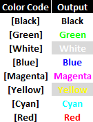
To specify the color for a section in the format code, type the name of one of the following eight colors in the code and enclose the name in square brackets as shown. The color code must be the first item in the code section.

[Black] [Blue] [Cyan] [Green] [Magenta] [Red] [White] [Yellow]

To indicate that a number format will be applied only if the number meets a condition that you have specified, enclose the condition in square brackets. The condition consists of a comparison operator and a value. For example, the following number format will display numbers that are less than or equal to 100 in a red font and numbers that are greater than 100 in a blue font.

[Red][<=100];[Blue][>100]

To hide zeros or to hide all values in cells, create a custom format by using the codes below. The hidden values appear only in the formula bar. The values are not printed when you print your sheet. To display the hidden values again, change the format to the General number format or to an appropriate date or time format.

To hide	Use this code
Zero values	0;–0;;@
All values	;;; (three semicolons)

Use the following keyboard shortcuts to enter the following currency symbols in the Type box.

To enter	Press these keys
¢ (cents)	OPTION + 4
£ (pounds)	OPTION + 3
¥ (yen)	OPTION + Y
€ (euro)	OPTION + SHIFT + 2

The regional settings for currency determine the position of the currency symbol (that is, whether the symbol appears before or after the number and whether a space separates the symbol and the number). The regional settings also determine the decimal symbol and the thousands separator. You can control these settings by using the Mac OS X International system preferences.

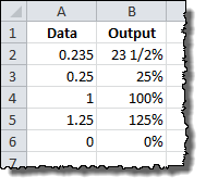
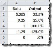
To display numbers as a percentage of 100 — for example, to display .08 as 8% or 2.8 as 280% — include the percent sign (%) in the number format.

To display numbers in scientific notation, use one of the exponent codes in the number format code — for example, E–, E+, e–, or e+. If a number format code section contains a zero (0) or number sign (#) to the right of an exponent code, Excel displays the number in scientific notation and inserts an «E» or «e». The number of zeros or number signs to the right of a code determines the number of digits in the exponent. The codes «E–» or «e–» place a minus sign (-) by negative exponents. The codes «E+» or «e+» place a minus sign (-) by negative exponents and a plus sign (+) by positive exponents.

To format dates and times, use the following codes.

Important: If you use the «m» or «mm» code immediately after the «h» or «hh» code (for hours) or immediately before the «ss» code (for seconds), Excel displays minutes instead of the month.

To display	As	Use this code
Years	00-99	yy
Years	1900-9999	yyyy
Months	1-12	m
Months	01-12	mm
Months	Jan-Dec	mmm
Months	January-December	mmmm
Months	J-D	mmmmm
Days	1-31	d
Days	01-31	dd
Days	Sun-Sat	ddd
Days	Sunday-Saturday	dddd
Hours	0-23	h
Hours	00-23	hh
Minutes	0-59	m
Minutes	00-59	mm
Seconds	0-59	s
Seconds	00-59	ss
Time	4 AM	h AM/PM
Time	4:36 PM	h:mm AM/PM
Time	4:36:03 PM	h:mm:ss A/P
Time	4:36:03.75 PM	h:mm:ss.00
Elapsed time (hours and minutes)	1:02	[h]:mm
Elapsed time (minutes and seconds)	62:16	[mm]:ss
Elapsed time (seconds and hundredths)	3735.80	[ss].00

Note: If the format contains AM or PM, the hour is based on the 12-hour clock, where «AM» or «A» indicates times from midnight until noon and «PM» or «P» indicates times from noon until midnight. Otherwise, the hour is based on the 24-hour clock.

Introduction

Number formats control how numbers are displayed in Excel. The key benefit of number formats is that they change how a number looks without changing any data. They are a great way to save time in Excel because they perform a huge amount of formatting automatically. As a bonus, they make worksheets look more consistent and professional.

Video: What is a number format

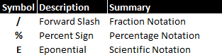
What can you do with custom number formats?

Custom number formats can control the display of numbers, dates, times, fractions, percentages, and other numeric values. Using custom formats, you can do things like format dates to show month names only, format large numbers in millions or thousands, and display negative numbers in red.

Where can you use custom number formats?

Many areas in Excel support number formats. You can use them in tables, charts, pivot tables, formulas, and directly on the worksheet.

Worksheet — format cells dialog
Pivot Tables — via value field settings
Charts — data labels and axis options
Formulas — via the TEXT function

What is a number format?

A number format is a special code to control how a value is displayed in Excel. For example, the table below shows 7 different number formats applied to the same date, January 1, 2019:

Input	Code	Result
1-Jan-2019	yyyy	2019
1-Jan-2019	yy	19
1-Jan-2019	mmm	Jan
1-Jan-2019	mmmm	January
1-Jan-2019	d	1
1-Jan-2019	ddd	Tue
1-Jan-2019	dddd	Tuesday

The key thing to understand is that number formats change the way numeric values are displayed, but they do not change the actual values.

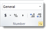
Where can you find number formats?

On the home tab of the ribbon, you’ll find a menu of build-in number formats. Below this menu to the right, there is a small button to access all number formats, including custom formats:

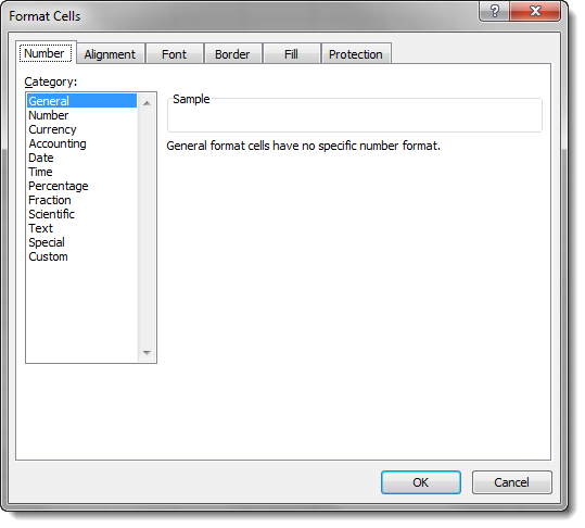
This button opens the Format Cells dialog box. You’ll find a complete list of number formats, organized by category, on the Number tab:

Note: you can open Format Cells dialog box with the keyboard shortcut Control + 1.

General is default

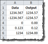
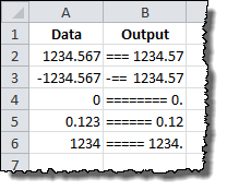
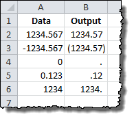
By default, cells start with the General format applied. The display of numbers using the General number format is somewhat «fluid». Excel will display as many decimal places as space allows, and will round decimals and use scientific number format when space is limited. The screen below shows the same values in column B and D, but D is narrower and Excel makes adjustments on the fly.

How to change number formats

You can select standard number formats (General, Number, Currency, Accounting, Short Date, Long Date, Time, Percentage, Fraction, Scientific, Text) on the home tab of the ribbon using the Number Format menu.

Note: As you enter data, Excel will sometimes change number formats automatically. For example if you enter a valid date, Excel will change to «Date» format. If you enter a percentage like 5%, Excel will change to Percentage, and so on.

Shortcuts for number formats

Excel provides a number of keyboard shortcuts for some common formats:

Format	Shortcut
General format	Ctrl Shift ~
Currency format	Ctrl Shift $
Percentage format	Ctrl Shift %
Scientific format	Ctrl Shift ^
Date format	Ctrl Shift #
Time format	Ctrl Shift @
Custom formats	Control + 1

See also: 222 Excel Shortcuts for Windows and Mac

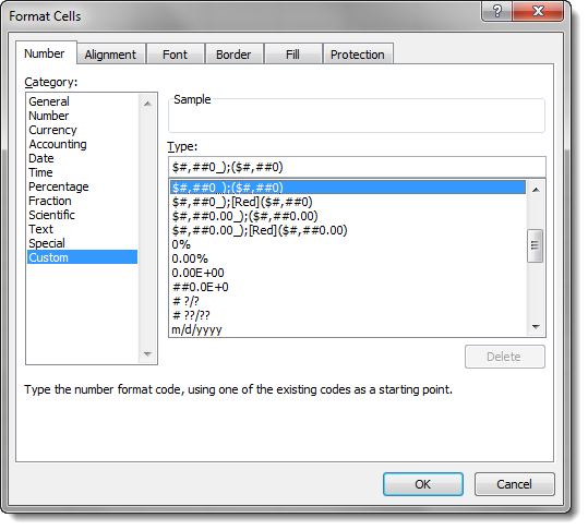
Where to enter custom formats

At the bottom of the predefined formats, you’ll see a category called custom. The Custom category shows a list of codes you can use for custom number formats, along with an input area to enter codes manually in various combinations.

When you select a code from the list, you’ll see it appear in the Type input box. Here you can modify existing custom code, or to enter your own codes from scratch. Excel will show a small preview of the code applied to the first selected value above the input area.

Note: Custom number formats live in a workbook, not in Excel generally. If you copy a value formatted with a custom format from one workbook to another, the custom number format will be transferred into the workbook along with the value.

How to create a custom number format

To create custom number format follow this simple 4-step process:

Select cell(s) with values you want to format
Control + 1 > Numbers > Custom
Enter codes and watch preview area to see result
Press OK to save and apply

Tip: if you want base your custom format on an existing format, first apply the base format, then click the «Custom» category and edit codes as you like.

How to edit a custom number format

You can’t really edit a custom number format per se. When you change an existing custom number format, a new format is created and will appear in the list in the Custom category. You can use the Delete button to delete custom formats you no longer need.

Warning: there is no «undo» after deleting a custom number format!

Structure and Reference

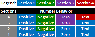
Excel custom number formats have a specific structure. Each number format can have up to four sections, separated with semi-colons as follows:

This structure can make custom number formats look overwhelmingly complex. To read a custom number format, learn to spot the semi-colons and mentally parse the code into these sections:

Positive values
Negative values
Zero values
Text values

Not all sections required

Although a number format can include up to four sections, only one section is required. By default, the first section applies to positive numbers, the second section applies to negative numbers, the third section applies to zero values, and the fourth section applies to text.

When only one format is provided, Excel will use that format for all values.
If you provide a number format with just two sections, the first section is used for positive numbers and zeros, and the second section is used for negative numbers.
To skip a section, include a semi-colon in the proper location, but don’t specify a format code.

Characters that display natively

Some characters appear normally in a number format, while others require special handling. The following characters can be used without any special handling:

Character	Comment
$	Dollar
+-	Plus, minus
()	Parentheses
{}	Curly braces
<>	Less than, greater than
=	Equal
:	Colon
^	Caret
‘	Apostrophe
/	Forward slash
!	Exclamation point
&	Ampersand
~	Tilde
	Space character

Escaping characters

Some characters won’t work correctly in a custom number format without being escaped. For example, the asterisk (*), hash (#), and percent (%) characters can’t be used directly in a custom number format – they won’t appear in the result. The escape character in custom number formats is the backslash (). By placing the backslash before the character, you can use them in custom number formats:

Value	Code	Result
100	#0	#100
100	*0	*100
100	%0	%100

Placeholders

Certain characters have special meaning in custom number format codes. The following characters are key building blocks:

Character	Purpose
0	Display insignificant zeros
#	Display significant digits
?	Display aligned decimals
.	Decimal point
,	Thousands separator
*	Repeat following character
_	Add space
@	Placeholder for text

Zero (0) is used to force the display of insignificant zeros when a number has fewer digits than zeros in the format. For example, the custom format 0.00 will display zero as 0.00, 1.1 as 1.10 and .5 as 0.50.

Pound sign (#) is a placeholder for optional digits. When a number has fewer digits than # symbols in the format, nothing will be displayed. For example, the custom format #.## will display 1.15 as 1.15 and 1.1 as 1.1.

Question mark (?) is used to align digits. When a question mark occupies a place not needed in a number, a space will be added to maintain visual alignment.

Period (.) is a placeholder for the decimal point in a number. When a period is used in a custom number format, it will always be displayed, regardless of whether the number contains decimal values.

Comma (,) is a placeholder for the thousands separators in the number being displayed. It can be used to define the behavior of digits in relation to the thousands or millions digits.

Asterisk (*) is used to repeat characters. The character immediately following an asterisk will be repeated to fill remaining space in a cell.

Underscore (_) is used to add space in a number format. The character immediately following an underscore character controls how much space to add. A common use of the underscore character is to add space to align positive and negative values when a number format is adding parentheses to negative numbers only. For example, the number format «0_);(0)» is adding a bit of space to the right of positive numbers so that they stay aligned with negative numbers, which are enclosed in parentheses.

At (@) — placeholder for text. For example, the following number format will display text values in blue:

0;0;0;[Blue]@

See below for more information about using color.

Automatic rounding

It’s important to understand that Excel will perform «visual rounding» with all custom number formats. When a number has more digits than placeholders on the right side of the decimal point, the number is rounded to the number of placeholders. When a number has more digits than placeholders on the left side of the decimal point, extra digits are displayed. This is a visual effect only; actual values are not modified.

Number formats for TEXT

To display both text along with numbers, enclose the text in double quotes («»). You can use this approach to append or prepend text strings in a custom number format, as shown in the table below.

Value	Code	Result
10	General» units»	10 units
10	0.0″ units»	10.0 units
5.5	0.0″ feet»	5.5 feet
30000	0″ feet»	30000 feet
95.2	«Score: «0.0	Score: 95.2
1-Jun	«Date: «mmmm d	Date: June 1

Number formats for DATES

Dates in Excel are just numbers, so you can use custom number formats to change the way they display. Excel has many specific codes you can use to display components of a date in different ways. The screen below shows how Excel displays the date in D5, September 3, 2018, with a variety of custom number formats:

Number formats for TIME

Times in Excel are fractional parts of a day. For example, 12:00 PM is 0.5, and 6:00 PM is 0.75. You can use the following codes in custom time formats to display components of a time in different ways. The screen below shows how Excel displays the time in D5, 9:35:07 AM, with a variety of custom number formats:

Note: m and mm can’t be used alone in a custom number format since they conflict with the month number code in date format codes.

Number formats for ELAPSED TIME

Elapsed time is a special case and needs special handling. By using square brackets, Excel provides a special way to display elapsed hours, minutes, and seconds. The following screen shows how Excel displays elapsed time based on the value in D5, which represents 1.25 days:

Number formats for COLORS

Excel provides basic support for colors in custom number formats. The following 8 colors can be specified by name in a number format: [black] [white] [red][green] [blue] [yellow] [magenta] [cyan]. Color names must appear in brackets.

Colors by index

In addition to color names, it’s also possible to specify colors by an index number (Color1,Color2,Color3, etc.) The examples below are using the custom number format: [ColorX]0″▲▼», where X is a number between 1-56:

[Color1]0"▲▼" // black
[Color2]0"▲▼" // white
[Color3]0"▲▼" // red
[Color4]0"▲▼" // green
etc.

The triangle symbols have been added only to make the colors easier to see. The first image shows all 56 colors on a standard white background. The second image shows the same colors on a gray background. Note the first 8 colors shown correspond to the named color list above.

Apply number formats in a formula

Although most number formats are applied directly to cells in a worksheet, you can also apply number formats inside a formula with the TEXT function. For example, with a valid date in A1, the following formula will display the month name only:

=TEXT(A1,"mmmm")

The result of the TEXT function is always text, so you are free to concatenate the result of TEXT to other strings:

="The contract expires in "&TEXT(A1,"mmmm")

The screen below shows the number formats in column C being applied to numbers in column B using the TEXT function:

One quirk of the TEXT function relates to double quotes («») that are part of certain custom number formats. Because the format_text is entered as a text string, Excel won’t allow you to enter the formula without removing the quotes or adding more quotes. For example, to display a large number in thousands, you can use a custom number format like this:

0, "k"

Notice k appears in quotes («k»). To apply the same format with the TEXT function, you can use simply:

=TEXT(A1,"0, k")

Notice the k is not surrounded by quotes. Alternately, you can add extra double quotes as below, which returns the same result:

=TEXT(A1,"0,""K""")

This behavior only occurs when you are hardcoding a format inside TEXT. If you are applying a format entered elsewhere on the worksheet (as in cells C6 and C9 in the worksheet above) you can use a standard number format.

Measurements

You can use a custom number format to display numbers with an inches mark («) or a feet mark (‘). In the screen below, the number formats used for inches and feet are:

0.00 ' // feet
0.00 " // inches

These results are simplistic, and can’t be combined in a single number format. You can however use a formula to display feet together with inches.

Conditionals

Custom number formats also up to two conditions, which are written in square brackets like [>100] or [<=100]. When you use conditionals in custom number formats, you override the standard [positive];[negative];[zero];[text] structure. For example, to display values below 100 in red, you can use:

[Red][<100]0;0

To display values greater than or equal to 100 in blue, you can extend the format like this:

[Red][<100]0;[Blue][>=100]0

To apply more than two conditions, or to change other cell attributes, like fill color, etc. you’ll need to switch to Conditional Formatting, which can apply formatting with much more power and flexibility using formulas.

Plural text labels

You can use conditionals to add an «s» to labels greater than zero with a custom format like this:

[=1]0″ day»;0″ days»

Telephone numbers

Custom number formats can also be used for telephone numbers, as shown in the screen below:

Notice the third and fourth examples use a conditional format to check for numbers that contain an area code. If you have data that contains phone numbers with hard-coded punctuation (parentheses, hyphens, etc.) you will need to clean the telephone numbers first so that they only contain numbers.

Hide all content

You can actually use a custom number format to hide all content in a cell. The code is simply three semi-colons and nothing else ;;;

To reveal the content again, you can use the keyboard shortcut Control + Shift + ~, which applies the General format.

Other resources

Developer Bryan Braun built a nice interactive tool for building custom number formats

Источник

If you used Excel in any shape or form, there is a pretty good chance that you’ve used the formatting and number formatting features. Formatting options like number, currency, percentage, date and time values are easily accessible to users. However, that’s not all there is in the world of text and number formatting. Going down the rabbit hole, custom formatting can help you fully configure Excel’s built-in settings for formatting.

The main advantage of this approach is that you can alter the look of your data without changing the actual values. This means that you do not need to use additional spaces or formulas to create the layout you want and preserve the raw data.

If you want to modify your data anyways, or need to change a value inside a formula, you can use the TEXT function with all custom formatting syntax we are going to cover in this article. It should be noted that the TEXT function returns a text, and the return value cannot be used in mathematical calculations. If you do, you will receive a #VALUE! error. In this article we’re going to be using a workbook template. You can download it below.

How to create a custom number format in Excel

Select the cell to be formatted and press Ctrl+1 to open the Format Cells dialog. An alternative way to do is by right-clicking the cell and then going to Format Cells > Number Tab.
Under Category, select Custom.
Type in the format code into the Type
Click OK to save your changes.

Note: In Format Cells dialog you can modify the built-in format codes by selecting the format you want to modify in its own category (i.e. Currency > ($1,234.10)) and then selecting Custom Category. Don’t worry, Excel will not let you delete built-in formats.

Basics

Syntax

The format code has 4 sections separated by semicolons.

POSITIVE; NEGATIVE; ZERO; TEXT

These sections are optional,

If a code contains only 1 section, the format is applied to all number types — positive, negative and zero.
If a code contains 2 sections, the first section is used for positive and zero values, while the second section is applied to negative values.
If a code contains 3 sections, the first is for positive, the second is for negative, and the third is for zero.
A code only affects text values if all sections exist.

Default format type in Excel is called General. You can type General for sections you don’t want formatted. Make sure you use a minus sign (-) with General if you want to skip negative values.

If you want to completely hide a type, leave it blank after the semicolon. For example; to hide 0 values, General;-General;;General

Placeholders and the Cheat Sheet

Placeholder	Description	Raw Value	Format Code	Formatted Value
General	Default format	1234.567	General	1234.567
#	Placeholder for digits (numbers) and does not add any leading zeroes.	1234.567	#####.####	1234.567
0	Placeholder for digits (numbers) and add any leading zeroes.	1234.567	00000.0000	01234.5670
?	Placeholder for digits (numbers) and add space characters.	1234.567	?????.????	1234.567
.	Placeholder for the decimal place.	1234.567	0.00	1234.57
_	Adds a blank space, to the width of the following character. You can use in combination with parentheses to add left and right indents, _( and _) respectively.	99	_(#_);(#)	99
-25	(25)
58	58
12	12
-71	(71)
36	36
*	Repeats the character after asterisk until the width of the cell is filled.	66	0 *!	66 !!!!!!!!!!!!!!!
Full Name	@ *_	Full Name ____
%	Convert value to a percentage with % sign	0.12	%	12%
,	Thousands separator	1234.567	#,	1
12345678	#,	12,346
12345678	#,###,	12,346
12345678	#,,	12
E	Scientific notation format. Requires a ‘+’ symbol after, and a digit placeholder before and after.	1234.567	0.00E+00	1.23E+03
/	Represents fractions	1.234	# ##/##	1 11/47
1.234	# 000/000	1 117/500
1.234	##/##	58/47
«»	Text placeholder for multiple characters	1234.567	#,##0 «km/h»	1,235 km/h
Good	«Result is: «@	Result is: Good
	Text placeholder for single character	1234	#.00, K	1.23 K
1234567	#.00,, M	1.23 M
@	Placeholder for text	Bad	«Result is: «@	Result is: Bad
[color]	Change Color of value. Options: [Black], [Green], [White], [Blue], [Magenta], [Yellow], [Cyan], [Red]	1234.567	[Green]#,##0.00_); [Red](#,##0.00); [Blue]0.00_); [Magenta]@	1,234.57
-1234.567	(1,234.57)
0	0.00
This is a text	This is a text

Common Practices

Display and control of the first digit and decimals

Decimal places in the code are indicated with a period (.). Number of zeroes after the period (.) define the number of decimal places. For example,

0 — display 1 decimal place
00 — display 2 decimal places

If the number has more decimals than the decimal placeholders defined, the number will be rounded to the nearest number of placeholders.

Raw Value	Format Code	Formatted Value
123.4	0.0	123.4
123.4	0.00	123.40
123.45	0.00	123.45
123.45	0.00	123.46
123.456	0.0	123.5

Alternatively, hash (#) and question mark (?) symbols can be used as decimal places. However, because any missing decimal places will be filled with zeroes, using zeroes instead will be easier to read.

Raw Value	Format Code	Formatted Value
0.25	0.00	0.25
0.25	#.##	.25
123	0.00	123.0
123	#.??	123.00
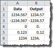
123	#.##	123.

Add text to numbers

Custom text can be added to the beginning or the end of a value. Text and characters should be added inside quotes («») and backslashes (). You can use backslash () to add single character.

Raw Value	Format Code	Formatted Value
123.4	0.0 «ft.»	123.4 ft.
123.4	0.00 l	123.40 l
123.45	«Approx.» 0	Approx. 123
123.45	«Result:» 0.00 C	Result: 123.46 C
Bad	«Result is: «@	Result is: Bad

Quotation marks or backslashes are not necessary for spaces ( ) and some special characters.

Symbol	Description
+ and —	Plus and minus signs
( )	Left and right parenthesis
:	Colon
^	Caret
‘	Apostrophe
{ }	Curly brackets
< >	Less-than and greater than signs
=	Equal sign
/	Forward slash
!	Exclamation point
&	Ampersand
~	Tilde
Space character

Below are some special characters you can use by copying or typing in the numerical code while pressing down Alt button.

Symbol	Code	Description
™	Alt+0153	Trademark
©	Alt+0169	Copyright symbol
°	Alt+0176	Degree symbol
±	Alt+0177	Plus-Minus sign
µ	Alt+0181	Micro sign

Hide value

If you leave any number of sections blank, the value of those sections will be hidden. A section should always be separated (defined) by a semicolon (;). Here are some examples,

Raw Value	Format Code	Formatted Value
1	0;;0;	1
-2	0;;0;
0	0;;0;	0
Some text	0;;0;
1	;(0);;@
-2	;(0);;@	(2)
0	;(0);;@
Some text	;(0);;@	Some Text
1	;;;
-2	;;;
0	;;;
Some text	;;;

Replace zeroes with dashes

Zeroes can make data tables look more complicated than they actually are. You can hide them completely by using the previous method, or replace them with any character of your choice. Dash (-) is a common example. All you need to is place a dash into the ‘Zero section’.

Raw Value	Format Code	Formatted Value
0	General;-General;»-«;General	—
3487	General;-General;»-«;»-«	—
12	#,##0.00;(#,##0.00);»-«;	—

Start with zeroes

If try to enter a ZIP number that starts with 0, the leading zeroes will be removed automatically by Excel. To keep the leading zeros, use zero (0) placeholder for whole numbers.

Raw Value	Format Code	Formatted Value
10010	00000	10010
3487	00000	03487
12	00000	00012
0	00000	00000
123456	00000	123456

Dealing with thousands, millions, and more

You may have noticed that ‘0.0’ or other simple formats do not separate thousands or millions. Adding a comma into the code will insert commas to separate numbers.

Raw Value	Format Code	Formatted Value
1234	#,##0	1,234
123456	#,##0	123,456
12345678	#,##0	12,345,678
123456.789	#,##0	123,457
123456.789	#,##0.0	123,456.8

There must be placeholders for numbers smaller than one thousand, otherwise such values will be hidden. This behavior allows us to round and format our value to show only thousands or millions.

Raw Value	Format Code	Formatted Value
1234	#,	1
123456	#,	123
12345678	#,	12345
12345678	#,,	12
123456	#.0, K	123.5 K
12345678	#.0,, M	12.3 M

Display numbers as phone numbers

Phone numbers can be hard to read without any separators. Custom Number Format Codes is perfect for this job. The hash (#) character should be your best bet to avoid any redundancy of placeholders (0, ?)

Raw Value	Format Code	Formatted Value
1234567890	(###) ###-####	(123) 456-7890
12345678900	(###) #### ####	(123) 4567 8900
1234567890	(##) #### ####	(12) 3456 7890

Showing Month and Weekday Names

Date and time values are stored as numbers in Excel. When you enter a date, Excel automatically converts it into a numerical value, and then formats the cell.

Before jumping into the code, let’s review some basics. Formatting code has special placeholders for date and time formatting that behave a bit differently. For example, while m and mm will show month as a number, mmm and mmmm will show as a text string. Below are some examples.

Raw Value	Format Code	Formatted Value
4/1/2018	m	4
4/1/2018	mm	04
4/1/2018	mmm	Apr
4/1/2018	mmmm	April
4/1/2018	mmmmm	A
4/1/2018	d	1
4/1/2018	dd	01
4/1/2018	ddd	Sun
4/1/2018	dddd	Sunday
4/1/2018 11:59:31 PM	dddd, mmmm dd, yyyy h:mm AM/PM;@	Sunday, April 01, 2018 11:59 PM

Here is the full list of options for the date 4/1/2018 23:59:31 ,

Format Code	Description	Example (4/1/2018 23:59:31)
yyyy	Displays the year as a four-digit number.	2018
yy	Displays the year as a two-digit number.	18
m	Displays the month as a number without a leading zero.	4
mm	Displays the month with a leading zero.	04
mmm	Displays the month as text, as an abbreviation.	Apr
mmmm	Displays the month as text.	April
mmmmm	Displays the month as a single character	A
d	Displays the day as a number, without a leading zero.	1
dd	Displays the day as a number, with a leading zero.	01
ddd	Displays the day as a day of the week, as an abbreviation.	Sun
dddd	Displays the day as a day of the week, without abbreviation	Sunday
h	Displays the hour without a leading zero.	23
hh	Displays the hour with a leading zero.	23
[h]	Displays elapsed time in hours (to be used when the time value exceeds 24 hours).	1036607
m	Displays the minute without a leading zero.	4
mm	Displays the minute with a leading zero.	04
[m]	Displays elapsed time in minutes (to be used when the time value exceeds 60 minutes).	62196479
s	Displays the second without a leading zero.	31
ss	with a leading zero.	31
[s]	Displays elapsed time in seconds (to be used when the time value exceeds 60 seconds).	3731788771
AM/PM	Converts to 12-hour time. Displays either AM/am/A/a or PM/pm/P/p depending on the time of day.	PM
am/pm	pm
A/P	P
a/p	p

Come in Colors Everywhere

Number Formatting can be used color sections of a code. A common example is using the color red for negative numbers. Color code must be placed inside square brackets (i.e. [color]), and entered at the beginning of a section. Here are some available colors,

[Black]
[Blue]
[Cyan]
[Green]
[Magenta]
[Red]
[White]
[Yellow]

Raw Value	Format Code	Formatted Value
1234.567	[Green]#,##0.00_);[Red](#,##0.00);[Blue]0.00);[Magenta]@	1,234.57
-1234.567	(1,234.57)
0	0.00
This is a text	This is a text

Conditions

Although Excel has conditional formatting menu, basic conditions can be applied through code. Condition should be placed inside square brackets (i.e. [condition]) just like colors. Conditions are similar to the conditions in some functions (i.e. SUMIF). First add a logical operator, and then a value. For example, “[>=1000000]” means “if value of cell is greater than or equal to 1,000,000 apply the following format”. Conditions should come before the actual code, again, just like with colors. If you want to a color as well, the color code should come first.

Another important thing to note here is, that section structure changes from Positive, Negative, Zero, Text to First Condition, Second Condition (if exists), if previous conditions are not applied. There should be at least two sections for conditions.

If you enter only one condition code and then save the format, Excel will automatically add the second section with «;General». This means that if the condition is not met, General format will be used.

Raw Value	Format Code	Formatted Value
1234567890	[>=1000000]#,##0,,»M»;[>=1000]#,##0,»K»;0	1,235M
12345	12K
1	[=1]0″ apple»;0″ apples»	1 apple
10	10 apples
25	[Green][>=85]»PASSED»;[Blue][>=60]»RE-CHECK»;[Red]»FAILED»	FAILED
72	RE-CHECK
91	PASSED

Источник

In Excel, you aren’t limited to using built-in number formats. You can define your own custom number formats to display values as thousands or millions (23K or 95.3M), add leading zeros, display » — » for zero values, make negative values red, add bullets, and much more.

This Article (bookmarks):

Watch the Video Overview
How to Create a Custom Number Format
Number Format Codes
Examples
- Format for Thousands and Millions
- Display Leading Zeros and Include Commas
- Display Units Without Converting to Text
- Special Time Formats
- Including Special Symbols
- Displaying Fractions
- Trailing and Leading Characters to Fill a Cell
- Chart Axes and Labels
Using Color Codes
Conditional Operators
Custom Location Codes for Dates

Watch the video we created to go along with this article!

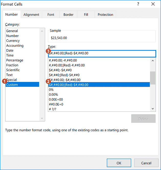
How to Create a Custom Number Format

To create a custom number format, it is easiest to begin with a built-in format. Open the Format Cells dialog box by pressing Ctrl+1 (or right-click on a cell and select Format Cells) and select the Number tab (see the image below). Then (1) Choose Custom from the Category list, (2) Select a built-in format similar to what you want, and (3) Edit the format string in the Type field.

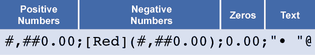
Number Format Codes

A number format string uses up to 4 different codes, separated by semicolons, as shown in the image below.

Instead of explaining the syntax in detail at this point, let’s take a look at some examples and learn as we go.

Some of the characters like #, 0, @, etc. have special meanings. Some codes like [Red] can change the font color, and quotes can be used to display text or special characters. The table below summarizes some of these special characters.

Special Characters in Number Formats

Character	Description
#	A digit placeholder
0	A digit that is to be displayed even if it is zero
,	(Comma) Interpreted as a 1000’s marker
@	Represents the value displayed as text
*	(Asterisk) Repeats the next character to fill the cell
[ColorCode]	See the section below about using color codes
[<=100]	Conditional operators (valid only in the Positive and Negative sections)
/	Used for fractions such as # #/12 or as the / character for dates
» «	(Quotes) Used to display whatever is contained within the quotes as text, such as 0.00 «feet»
d or dd ddd dddd	Day number (0-31 or 00-31) Abbreviated day of week (Mon, Tue, etc.) Full day of week (Monday, Tuesday, etc.)
m or mm mmm mmmm mmmmm	Month number (0-12 or 00-12) Abbreviated month name (Jan, Feb, etc.) Full month name (January, February, etc.) First letter of the month (J, F, M, etc.)
y or yy yyyy	Year (0-99 or 00-99) Full year (1900-9999)
h or hh m or mm s or ss	Hour (0-23 or 00-23) Minutes (0-59 or 00-59) Seconds (0-59 or 00-59)

NOTE Some characters are specific to locale/language settings. For example J is used for Year in some countries.

Custom Number Format Examples

The examples below show some of the custom number formats that I’ve found the most useful. This isn’t a comprehensive list of all possible number formats. See support.microsoft.com to search for other articles on this subject.

TIP Using a custom number format only affects the displayed value. A formula that references the cell will use the stored value no matter how it is displayed. This means you can still use a formula to refer to the value even though the number might be displayed as «12 ft.»

To see these examples in action, download the Excel file below.

Download the Example File (CustomNumberFormats.xlsx)

Custom Number Format for Thousands and Millions

Format Code	Value	Displayed As	Description
0,K 0.0,K 0.0, «Thousand»	23543	24K 23.5K 23.5 Thousand	Display values in thousands, using the letter K to indicate thousands. The «K» is just a displayed character — it has no special meaning in the number format string. If you want to display more than one letter, you need to enclose the characters in quotes, like the «Thousand» example.
0,,»M» 0.0,,»M» 0.0,, «Million»	23543000	24M 23.5M 23.5 Million	Display values in millons, using the letter M to indicate millions. Note that in this case, you need two commas.

NOTE These are very useful for chart axes and labels.

Display Leading Zeros and Include Commas

Format Code	Value	Displayed As	Description
000 00000	50.8	051 00051	Display values with leading zeros. This does not convert the value to text — it is only a display format.
#,##0.0	3543.46	3,543.5	Display values using commas to separate thousands, millions, etc. The # sign is used as a placeholder, meaning that if there are no 10’s, 100’s, or 1000’s, don’t display them.

Display Units Without Converting to Text

Format Code	Value	Displayed As
• Display a number and text in the same cell using the conditions [=1] and [>1]. The value is stored as a number, so you can still do calculations on the number of people.
[=1]# «person»;[>1]# «people»;0	1 5 0	1 person 5 people 0
• Display a number and text in the same cell. The value is stored as a number, so you can still do calculations.
0.0 «ft» 0.0 «kg» # #/## «in»	2.2 4.5 6.25	2.2 ft 4.5 kg 6 1/4 in
• Display a numeric YYMMDD value in years, months, days.
##»y» ##»m» ##»d»	360712	36y 07m 12d

Special Time Formats

There are quite a few built-in time formats to choose from. The following may be less known.

Format Code	Value	Displayed As	Description
[h]:mm:ss [h]:mm [mm]:ss [ss]	49:03:47	49:03:47 49:03 2943:47 176627	Shows elapsed time in hours, minutes or seconds. Note that time does not round up.
h:mm A/P h:mm a/p	2:25 PM	2:25 P 2:25 p	Displays time using «a» for AM and «p» for PM. Useful when trying to minimize column widths without making fonts smaller.

Including Special Symbols

Some ascii and unicode characters can be copied and pasted directly into the format code. This can be handy for displaying the degrees symbol for temperatures as well as other tricks like showing up and down arrows or bulleted lists.

Format Code	Value	Displayed As	Description
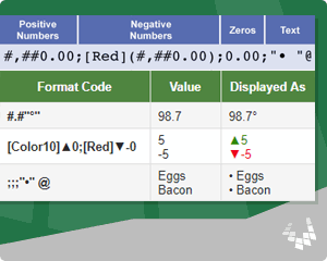
#.#»°»	98.7	98.7°	Display temperature in degrees with the ° symbol.
[Color10]▲0;[Red]▼-0	5 -5	▲5 ▼-5	Display special symbols for positive and negative, combined with colors.
;;;»•» @	Eggs Bacon	• Eggs • Bacon	Create a bulleted list using a special symbol for the bullet. When you enter text, the bullet will be displayed. Numbers and zero values will not be displayed.

Displaying Fractions

Format Code	Value	Displayed As	Description
# ??/12	5.75 12.5	5 9/12 12 6/12	Display a decimal number of feet as feet and inches (rounded to the nearest inch). Or display a decimal year in terms of years and months.
# ??/100	5.2 5.05 12.81	5 20/100 5 5/100 12 81/100	Using ??/100 will help line up values in a column (as opposed to just using ?/100). Note that fractions are automatically rounded.
?/2	5.2	10/2	Displays a simple fraction as numerator/denominator.

Trailing and Leading Characters to Fill a Cell

The asterisk (*) in a format code repeats the following character to fill the width of the cell.

Format Code	Value	Displayed As	Description
— @ *-	✁	— ✁ —————-	Trailing characters.
*.@	pg 2	………………pg 2	Leading characters

Custom Number Formats for Chart Axes and Labels

Format Code	Value	Displayed As	Description
0 «AD»;0 «BC»	247 -600	247 AD 600 BC	AD and BC Years. Use negative numbers for BC years and positive numbers for AD years.
mmm{Ctrl+j}yyyy	8/20/18	Aug 2018	Add a Carriage Return within the custom number format (e.g. between dddd and mmm) by pressing Ctrl+j.
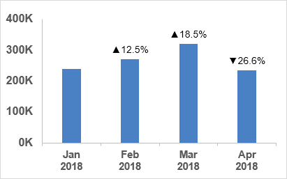
[Color10]▲0.0%;[Red]▼-0.0%	15.23% -23.57%	▲15.2% ▼-23.6%	Display arrows for positive and negative, combined with colors and percentages.

A couple of these examples can be seen in the image below. However, notice that the data labels don’t use color codes, so the percentages are shown only as black text rather than red and green. Too bad. Maybe Microsoft will fix that some day.

NOTE Editing a custom number format that contains a carriage return is tricky because you can’t see the second row. This is why I write out the code first using «{Ctrl+j}» or just «{j}» and then delete the «{j}» and press Ctrl+j in its place.

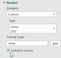
When adding a custom number format using the Format Axis window pane, you may not be able to press Ctrl+j to add a carriage return. In that case, first edit the format of the data source, then click on the Link to Source box as shown in the image to the right. After doing that, you can uncheck the Link to Source box and modify the original data source formatting.

Other Tricks

Format Code	Value	Displayed As	Description
;;;	anything		Display nothing, regardless of the value.
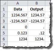
0.#	2	2.	Display a decimal point without a 0 after the decimal (2. instead of 2.0)
???.???	1.2 12.3 123.456	1.2 12.3 123.456	Vertically align the decimal point when displaying a column of numbers.

NOTE If you are looking for format codes for phone numbers, social security numbers, or zip codes, look in the Special category within the list of built-in number formats.

Custom Number Format Color Codes

By using color format codes such as [Red] or [Blue] or [Color10], you have a limited ability to alter the color of the font via custom number formats. The most common use I’ve seen is to color negative values red. However, one of the examples above also shows how you might want to use a green arrow.

Even though a new color palette was introduced in Excel 2007, the color codes for custom number formats are still based on the old color palette for the Excel 97-2003 format. I created the graphic below to provide a quick reference.

I made the above color code reference match the layout of the old color palette because there is not a consistent pattern to the numbering.

Define Your Own Color: You can modify the color palette in newer versions of Excel by going to File > Options > Save > Colors. This allows you to change the color associated with the Color1 through Color56 codes. This means that Color10 might not always be a dark green. If you purposely change the color palette (or somebody else does), Color10 might be some other color.

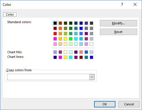
Excel 2016: File > Options > Save > Colors

NOTE The Color1-56 codes in Google Sheets are fixed colors and aren’t changed when you upload an Excel file with a customized color palette.

Conditional Operators

Conditional operators such as [<100] can be used to change the formatting in cases where positive;negative;0 is not how you want the divisions defined.

For example, the following format will display numbers less than 10 red, numbers between 10 and 20 green, other numbers blue, and text will be displayed based on the cell’s font color: [Red][<10]0.00;[Green][<=20]0.00;[Blue]0.00;@

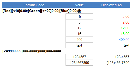
You are limited to 2 numeric conditions, which you place in the negative and positive sections of the format code.

Another use of conditional operators is to display phone numbers with and without an area code, depending on how many digits are in the phone number like this: [<=9999999]###-####;(###)###-####. This assumes that the phone numbers are entered as numbers and not text values. Meaning, that if you actually enter 123-1234 into a cell in Excel, it will be interpreted as a text value, not a number. The phone number format will display 1234567 to 123-4567 and it will display 1234567890 to (123)456-7890.

Custom Location Codes for Dates

When displaying month names and weekday names for dates, you can use location codes such as [$-fr-CA] at the beginning of the format code to tell Excel to display the names in other languages. To learn what the code is for a specific language and location, use the Format Cells dialog in Excel, choose one of the built-in Date formats, then choose the Locale (location) from the drop-down list. Then you can return to the Format Cells dialog box and click on the Custom tab to see what location code was added.

Format Code	Value	Displayed As	Language/Location
[$-en-US](ddd) mmm d, yyyy	10/1/2018	(Mon) Oct 1, 2018	English (United States)
[$-fr-CA](ddd) mmm d, yyyy	8/1/2018	(mer.) août 1, 2018	French (Canada)
[$-de-DE](ddd) mmm d, yyyy	10/1/2018	(Mo) Okt 1, 2018	German (Germany)

Other Notes About Custom Number Formats

To delete a custom number format, open the Format Cells dialog box, select the custom format from the list, then click Delete. When you delete a custom number format, all values in your workbook that use that format will revert to the General format.

Custom number formats that you create are saved with the file. If you want to use the custom format in a different file, you can copy/paste the formatting from your other file by copying and pasting the formatted cell or using the Format Painter tool.

References

Number Formats for Charts by Jon Peltier, Excel MVP
Excel Custom Number Format Guide by Mynda Treacy, Excel MVP

Источник

My column headings are labeled with numbers instead of letters

On the Excel menu, click Preferences.
Under Authoring, click General .
Clear the Use R1C1 reference style check box. The column headings now show A, B, and C, instead of 1, 2, 3, and so on.

Contents

1 How do you change Excel to Numbers?
2 How do I show column numbers in Excel?
3 How do I convert text to values in Excel?
4 How do I convert a column of numbers to column names in Excel?
5 How do I change the number format in Excel?
6 Why does Excel have numbers for columns?
7 How do I show columns and row numbers in Excel?
8 How do I get columns and row numbers in Excel?
9 How do I get row numbers in Excel?
10 How do I format numbers in Excel?
11 What are the different ways in formatting numbers?
12 How do I change the column title in Excel?
13 How do I change rows and column names in Excel?
14 How do I change Excel columns from numbers to alphabets?
15 How do I get rid of column 1 headers in Excel?
16 How do I change the row numbers in Excel?
17 What is an Xlookup in Excel?
18 Why can’t I see row numbers in Excel?
19 How do I add a numbered list in Excel?
20 How do I automatically number in sheets?

Change numbers with text format to number format in Excel for the…

Select the cells that have the data you want to reformat.
Click Number Format > Number. Tip: You can tell a number is formatted as text if it’s left-aligned in a cell.

How do I show column numbers in Excel?

Show column number

Click File tab > Options.
In the Excel Options dialog box, select Formulas and check R1C1 reference style.
Click OK.

How do I convert text to values in Excel?

Use the Format Cells option to convert number to text in Excel

Select the range with the numeric values you want to format as text.
Right click on them and pick the Format Cells… option from the menu list. Tip. You can display the Format Cells…
On the Format Cells window select Text under the Number tab and click OK.

How do I convert a column of numbers to column names in Excel?

To convert a column number to an Excel column letter (e.g. A, B, C, etc.) you can use a formula based on the ADDRESS and SUBSTITUTE functions. With this information, ADDRESS returns the text “A1”.

How do I change the number format in Excel?

You can use the Format Cells dialog to find the other available format codes:

Press Ctrl+1 ( +1 on the Mac) to bring up the Format Cells dialog.
Select the format you want from the Number tab.
Select the Custom option,
The format code you want is now shown in the Type box.

Why does Excel have numbers for columns?

Cause: The default cell reference style (A1), which refers to columns as letters and refers to rows as numbers, was changed. Solution: Clear the R1C1 reference style selection in Excel preferences. On the Excel menu, click Preferences.The column headings now show A, B, and C, instead of 1, 2, 3, and so on.

How do I show columns and row numbers in Excel?

On the Ribbon, click the Page Layout tab. In the Sheet Options group, under Headings, select the Print check box. , and then under Print, select the Row and column headings check box .

How do I get columns and row numbers in Excel?

It is quite easy to figure out the row number or column number if you know a cell’s address. If the cell address is NK60, it shows the row number is 60; and you can get the column with the formula of =Column(NK60). Of course you can get the row number with formula of =Row(NK60).

How do I get row numbers in Excel?

Use the ROW function to number rows

In the first cell of the range that you want to number, type =ROW(A1). The ROW function returns the number of the row that you reference. For example, =ROW(A1) returns the number 1.
Drag the fill handle. across the range that you want to fill.

How do I format numbers in Excel?

Formatting the Numbers in an Excel Text String

Right-click any cell and select Format Cell.
On the Number format tab, select the formatting you need.
Select Custom from the Category list on the left of the Number Format dialog box.
Copy the syntax found in the Type input box.

What are the different ways in formatting numbers?

How to change number formats. You can select standard number formats (General, Number, Currency, Accounting, Short Date, Long Date, Time, Percentage, Fraction, Scientific, Text) on the home tab of the ribbon using the Number Format menu. Note: As you enter data, Excel will sometimes change number formats automatically.

How do I change the column title in Excel?

Select a column, and then select Transform > Rename. You can also double-click the column header. Enter the new name.

How do I change rows and column names in Excel?

Rename columns and rows in a worksheet

Click the row or column header you want to rename.
Edit the column or row name between the last set of quotation marks. In the example above, you would overwrite the column name Gold Collection.
Press Enter. The header updates.

How do I change Excel columns from numbers to alphabets?

To change the column headings to letters, select the File tab in the toolbar at the top of the screen and then click on Options at the bottom of the menu. When the Excel Options window appears, click on the Formulas option on the left. Then uncheck the option called “R1C1 reference style” and click on the OK button.

How do I get rid of column 1 headers in Excel?

Go to Table Tools > Design on the Ribbon. In the Table Style Options group, select the Header Row check box to hide or display the table headers. If you rename the header rows and then turn off the header row, the original values you input will be retained if you turn the header row back on.

How do I change the row numbers in Excel?

Here are the steps to use Fill Series to number rows in Excel:

Enter 1 in cell A2.
Go to the Home tab.
In the Editing Group, click on the Fill drop-down.
From the drop-down, select ‘Series..’.
In the ‘Series’ dialog box, select ‘Columns’ in the ‘Series in’ options.
Specify the Stop value.
Click OK.

What is an Xlookup in Excel?

Use the XLOOKUP function to find things in a table or range by row.With XLOOKUP, you can look in one column for a search term, and return a result from the same row in another column, regardless of which side the return column is on.

Why can’t I see row numbers in Excel?

In order to show (or hide) the row and column numbers and letters go to the View ribbon. Set the check mark at “Headings”. That’s it!

How do I add a numbered list in Excel?

Click the Home tab in the Ribbon. Click the Bullets and Numbering option in the new group you created. The new group is on the far right side of the Home tab. In the Bullets and Numbering window, select the type of bulleted or numbered list you want to add to the text box and click OK.

How do I automatically number in sheets?

Use autofill to complete a series

On your computer, open a spreadsheet in Google Sheets.
In a column or row, enter text, numbers, or dates in at least two cells next to each other.
Highlight the cells. You’ll see a small blue box in the lower right corner.
Drag the blue box any number of cells down or across.

Источник

Excel has a lot of built-in number formats, but sometimes you need something specific. Whether you’re representing a little-used currency, tracking in-stock units, or want to color code profits and losses, you are in need of a an Excel custom number format. Number formatting in Excel is pretty powerful but that means it is also somewhat complex. This is the definitive guide to Excel’s custom number formats…

By default, each cell is formatted as “General”, which means it does not have any special formatting rules. When you enter data in a cell, Excel tries to guess what format it should have. When it doesn’t guess correctly, you need to change the format. Excel has a few pre-set formatting options attached to buttons in the Home menu, but if those don’t meet your needs, you need to use the full options available in the Format Cells menu.

To access this menu, look for the Number section of the Home menu tab. Click the arrow in the lower right corner of the Number section.

It will bring up the Format Cells menu in the Numbers tab:

Underneath the pre-defined number formats for common items like currency and percentage, there is a category called Custom. The format types in this section are different from the pre-set options. They are filled with symbols and codes:

A number format code is entered into the Type field in the Custom category. These codes are the key to creating any custom number format in Excel. First, however, we need to understand how they work…

Understanding the Number Format Codes

Number format codes are the string of symbols that define how Excel displays the data you store in cells. We will get into the ways to describe the formats in a minute, but first we need to go over how Excel interprets those symbols. Each number format code is made up of as many as 4 sections separated by a semi-colon (;).

These sections control formatting for one or more parts of the number line, including positive numbers, negative numbers, and zeros. They can also control formatting for sub-sets of these parts, like all numbers greater than 100 and text-based data. What each section controls depends on how many sections there are in the number format code. A full number format code will be entered as follows:

Section1;Section2;Section3;Section4

The behavior of different parts of the number line will be as follows:

As indicated above, when there is just one section provided, it describes the format for all numbers. With two, the first section describes the format of positive, zero, and text values, while the second section describes the format of negative values, etc.

You can choose to skip formatting for any of the middle sections by entering General instead of other format data. For example, if you only want to affect positive numbers and text, you can enter a number format code with this arrangement:

Section1;General;General;Section4

General strips all formatting from the data entered, so be careful how you use it. Negative numbers with the General format code will not display the minus sign in front of their number.

Important note: Using a single section number format code does not always have the same result as expanding the same rules to all sections. For example:

Section1

Is not the same as:

Section1;Section1;Section1;Section1

Look at the examples below to see examples of the difference…

Now that we understand what a number format code is, what can we do with it?

Changing Font Color with Number Format Codes

One of the simplest things you can do with number format codes is change the color of the font in the affected cells. The syntax for doing so is simple:

[Color Name]

Just choose the section that corresponds to the part of the number line you want to change color, and provide the color in brackets. The color options are as follows (the background is gray for contrast in the table, but backgrounds are not affected by the number format code):

As an example, we can provide a separate color code for each part of a number format code:

[Red]General;[Blue]General;[Magenta]General;[Cyan]General

The General message just tells Excel to represent the numbers as entered by the user. The output of this number format code looks like this:

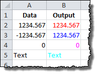
Note that the negative number in row 3 does not automatically get a negative sign (-) in front of it. We are overriding the default format of negative numbers in the cell. Also notice that the color format is not affecting anything about the presentation; the number of decimal places stays the same, as does the alignment of the data to the left or right of the cells.

Adding Text with Number Format Codes

You can add text around numbers with number format codes by inserting the text in a section one of two ways:

Single Characters

For single characters (like an @ symbol before a number), type a backslash () followed by the symbol. The number format code:

@General

Results in the following output:

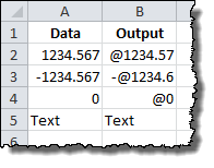
Note that the minus sign still precedes the negative number. Also note that the Text value is not affected by the @ symbol addition.

Importantly, this is different from the result if we expanded our format guideline to each section of the number format code:

@General;@General;@General;@General

Results in the following output:

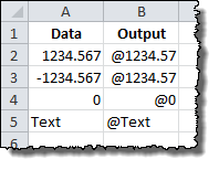
Note that the minus sign is gone from the negative number and the Text value now receives the @ symbol.

Text Strings

To add an entire text string to a number (like adding “units” to the end of a number), we surround the text string in quotation marks (” “). The number format code:

General" units"

Results in the following output:

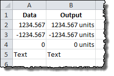
Once again, this is different from:

General" units";General" units";General" units";General" units"

Which results in:

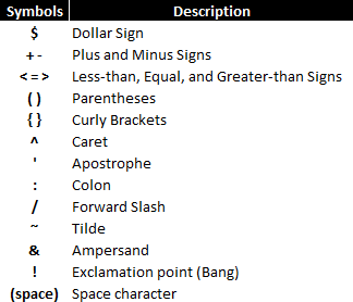
Special Characters

In addition to these two methods, there is a set of special symbol characters that do not need a leading backslash or quotes to be included in the number format code. The list is as follows:

Excel will also accept most other non-mathematical symbols, such a non-dollar currency symbols, copyright/trademark symbols, and Greek letters. These symbols are not available on most standard keyboards, but they can be entered by holding down the ALT key while typing in a four-digit number. Some of the most useful ones are below:

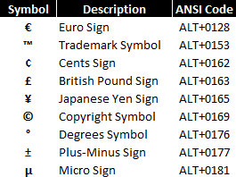
A full list of ANSI character codes can be found on Wikipedia here.

Changing Decimal Places, Significant Digits, and Commas

Adding symbols and colors is useful, but most of the work you’ll likely need to do with custom number formats is change the way Excel displays the numbers it stores. Number format codes use a set of symbols to represent how the data should appear in the cell. Here is a summary of the symbols:

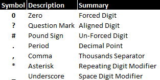
Let’s review them each in turn…

Zero (0)

Zeros in the number format code represent a forced digit. That means that whether or not the digit is relevant to the value, it will be shown. A great example of this is the standard dollars and cents notation that is used to represent prices in the United States: $0.00. Even if there are no extra cents in the amount, the two zeroes are still shown in the notation.

Here is an example of the zero code in action. The following examples are using this number format code:

0.00

Question Mark (?)

Question marks in the number format code represent an alignment digit. This means that when the number being shown doesn’t need the digit in question, a blank space of the same size is used. This is used to align decimal and comma places for more easy ranking of values, etc.

Here is an example of the question mark code in action. The following examples are using this number format code:

0.??

Pound Sign (#)

Sometimes called a hash mark, the pound sign in the number format code represents an optional digit. This means that when the number being shown doesn’t need the digit in question, it will be omitted from the displayed number. This is most often used to represent numbers in their most easily readable form.

Here is an example of the pound sign code in action. The following examples are using this number format code:

#.##

Period (.)

The period in the number format code represents the location of the decimal point in the number being displayed. When paired with the comma code, it can show numbers in thousands or millions, changing 1,200 to 1.2, for example. It is similar to the text format codes above in that it is always displayed when it is part of the number code, even when number being displayed does not straddle the decimal point. See the comma, pound sign and question mark examples above for useful illustrations of the period in use.

Comma (,)

The comma in the number format code represents the thousands separators in the number being displayed. It allows you to describe the behavior of digits in relation to the thousands or millions digits.

Here is an example of the comma code in action. The following examples are using this number format code:

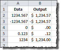
$??,???.00

Asterisk (*)

The asterisk in the number format code represents the repeating character modifier. It is used along with a character to display a repeating digit that fills the empty space in a cell.

Here is an example of the asterisk code in action. The following examples are using this number format code:

*=0.##

Underscore (_)

The underscore in the number code represents the space character modifier. It is used along with a character to display a blank space equal in size to the specified character. It can be used, for example, to properly align positive and negative numbers when parentheses are used in only the negative case.

Here is an example of the underscore code in action. The following examples are using this number format code:

_(#.##_);(#.##)

Using Fractions, Percentages, and Scientific Notation

Certain types of notation require that symbols be used to indicate the format change, including fractions, percentages, and scientific notation. Here is a summary of the symbols for each:

We’ll examine each in detail…

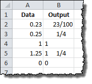
Fractions (/)

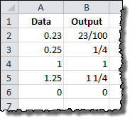
Fractions are special, since they require a change in units. The number 0.23 is represented as 23/100, but 0.25 can be simplified t0 1/4 or shown as 25/100. Similarly, 1.25 can be shown as 1 1/4 or the improper fraction 5/4. Which way Excel displays the number depends on how you construct the number format code.

Fractions effectively round values to the nearest possible fraction. They also take the guidelines of the pound sign and question mark symbols they are paired with.

Integer with Reduced Fractions

A fairly typical representation for fractions is to keep the whole numbers independent from the fraction remainder. The representation for this is relatively straightforward and can be done with pound signs and question marks to slightly different effect…

Using question mark (?) notation, the following number format code:

# ???/???

Produces a fraction remainder with up to three digits:

The alignment of the fraction bar is preserved regardless of the number of digits in use. If we limit the number of digits on each side of the fraction to 2, Excel will round the number to the nearest fraction value. The following number code format:

# ??/??

Changes the representation of 0.23 from 23/100 to 3/13.

If you don’t wish to preserve the alignment around the fraction bar, you can use a similar fraction number format code that uses pound signs.

Using pound sign notation, the following number format code:

# ###/###

Produces a more readable fraction remainder that can be justified or centered in the cell:

Improper Fractions

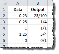
If you’d rather bundle the whole number portion of a value into the fraction itself, you can specify as much in the number format code.

Using pound sign notation, the following number format code:

###/###

Produces an improper fraction with up to three digits:

Fixed Base Fractions

It is also possible to force Excel to round fractions to a specific denominator by specifying it in the number format code.

Here is an example of a fixed base code in action. The following examples are using this number format code:

# ##/15

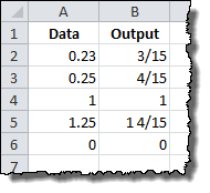
The result is a rounded fraction remainder that goes to the nearest number of 15ths.

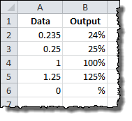
Percentages (%)

Much like fractions, percentages are controlled by the number format codes that accompany them. A basic percentage can be achieved with a pound sign symbol in the number format code:

#%

Results in the following output:

You can also specify fractional percentages, as shown with this number format code:

# #/#%

Results in single-digit fractions in the percentages where needed:

Finally, as always, you can specify the number of significant digits with decimal places:

#.0%

Results in a 10th place aligned decimal:

Scientific Notation (E)

It’s difficult to read extremely small and extremely large numbers conventionally because of all the leading and trailing zeroes. Scientific notation fixes that by moving the decimal to the relevant digits, so 0.0000001 can become 1 x 10^-7. Excel uses the E notation for this, so that same number would be 1E-07. So, as you’d expect, the capital letter E signals scientific notation in number format code.

Otherwise, scientific notation in Excel is controlled by the same number codes as percentages and fractions. It needs a number format code in front of the E to describe the relevant digits and a plus (+) and another number format code behind to describe the handling of the exponential digit.

Here is an example of a scientific notation code in action. The following examples are using this number format code:

#E+#

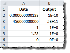
You can also achieve more consistent notation with zeros. The following examples are using this number format code:

0.00E+00

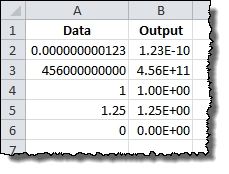
Note that in this case, the decimal and exponent are both constrained to 2 significant digits, regardless of whether they are necessary. The trade-off is, it keeps the output far more consistent, with a predictable string length.

Dates and Times

Dates and times in Excel are a special case. For a detailed discussion of how Excel uses them, please review the Definitive Guide to Using Dates and Times in Excel. The number format codes work identically to the format_text input for the TEXT command, and they can be reviewed here.

Get the latest Excel tips and tricks by joining the newsletter!

Andrew Roberts has been solving business problems with Microsoft Excel for over a decade. Excel Tactics is dedicated to helping you master it.

Join the newsletter to stay on top of the latest articles. Sign up and you’ll get a free guide with 10 time-saving keyboard shortcuts!

Что такое числовой формат?

Числовые форматы определяют способ отображения чисел в Excel. Ключевым их преимуществом является то, что они меняют внешний вид данных в ячейках без их изменения. В качестве бонуса они делают рабочие листы более наглядными и профессиональными.

Числовой формат – это специальный код для управления показом значения в Excel. Например, в таблице ниже показаны 7 различных способов отображения, применяемых к одной и той же дате, 1 января 2021 года:

Значение	Код формата	Результат
1-янв-2021	гггг г.	2021 г.
1-янв-2021	гг	21
1-янв-2021	ммм	Янв
1-янв-2021	мммм	Январь
1-янв-2021	д	1
1-янв-2021	ддд	Пт
1-янв-2021	дддд	пятница

Важно понимать, что числовые форматы меняют способ отображения значений, но не меняют фактические значения.

Форматированный результат — это просто то, как он выглядит. И вы должны быть осторожны, если используете эти обработанные результаты в вычислениях, которые не ссылаются непосредственно на ячейку. Например, если вы введете эти форматированные значения в калькулятор, вы получите результат, отличный от формулы, которая ссылается на эту ячейку. Часто это бывает при подсчёте итогов и суммы процентных долей.

Где найти числовые форматы?

На главной вкладке ленты вы найдете меню встроенных числовых форматов. Под этим меню справа есть небольшая кнопка для доступа ко всем ним, включая пользовательские:

Эта кнопка открывает диалоговое окно. Вы увидите полный список числовых форматов, упорядоченный по категориям, на вкладке «Число»:

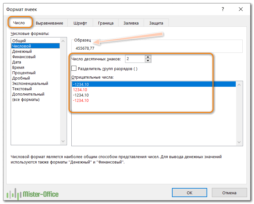
Примечание. Вы можете открыть это диалоговое окно с помощью сочетания клавиш Ctrl + 1.

По умолчанию.

По умолчанию ячейки в вашей рабочей книге представлены в формате Общий. Это означает, что Excel будет отображать столько десятичных знаков, сколько позволяет свободное пространство. Он будет округлять десятичные дроби и использовать формат научных чисел (экспоненциальный), когда свободного места для них недостаточно.

На приведенном ниже скриншоте показаны одни и те же значения в столбцах B и D, но D более узкий, и Excel вносит корректировки в представляемые данные буквально «на лету».

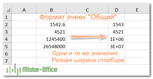
Как изменить формат чисел

Вы можете выбрать стандартные числовые форматы (Общий, Число, Денежный, Финансовый, Краткая дата, Длинная дата, Время, Процент, Дробь, Экспоненциальный, Текст) на главной вкладке ленты.

Более подробно о смене форматов, автоматическом их изменении, способах копирования, настройке отдельных параметров отображения — читайте в этой статье.

Быстрые клавиши для числовых форматов

В Excel есть несколько сочетаний клавиш для наиболее распространенных представлений:

Формат	Комбинация клавиш
Общий	Ctrl Shift ~
Валюта	Ctrl Shift $
Процент	Ctrl Shift %
Научный (экспоненциальный)	Ctrl Shift ^
Дата	Ctrl Shift #
Время	Ctrl Shift @

Где вводить пользовательские форматы?

Чтобы создать собственный формат Excel, откройте книгу, в которой вы хотите применить и сохранить его, и выполните следующие действия:

Выберите ячейку, для которой вы хотите создать уникальное оформление, и нажмите Ctrl + 1, чтобы открыть диалоговое окно «Формат ячеек».
В списке выберите «Все форматы».
Введите код формата в поле Тип.
Нажмите ОК, чтобы сохранить то, что вы создали.

При изменении существующего числового формата создается новый, который отображается в списке в категории «Все форматы». Вы можете использовать кнопку «Удалить», чтобы убрать те из них, которые вам больше не нужны.

Подождите, но что означают все эти символы в поле Тип? И как мне сложить их в правильную комбинацию, чтобы числа отображались так, как я хочу? Ну, это то, о чем остальная часть этого урока

Из чего состоит числовой формат Excel?

Чтобы иметь возможность создать свой новый формат в Excel, важно понимать, по каким правилам его нужно описать.

Вот пример кода настраиваемого формата Excel:

Код этот состоит из 4 разделов, отделённых друг от друга точкой с запятой. Они расположены в следующем порядке:

Для положительных чисел (отображение 2 десятичных знаков и разделителя тысяч).
Для отрицательных чисел (например, такой же, как для положительных, но заключен в круглые скобки).
Как показывать нули (например, отображать тире вместо нуля).
Представление текстовых значений (отображение текста определённым цветом).

Если указан только один код, то Excel будет использовать его для всех значений.

Если вы использовали только два раздела, то первый из них используется для положительных чисел и нулей, а второй предназначается для отрицательных значений.

Когда предоставлены первые три раздела, Excel будет использовать указанные правила отображения, а текст будет показан в том виде, в каком он был введен.

Чтобы пропустить раздел, поставьте точку с запятой в нужном месте, но больше ничего не пишите.

Правила форматирования Excel

При создании собственного числового формата в Excel помните следующие правила:

Он изменяет только визуальное представление, то есть способ отображения значения в ячейке. Базовое значение, хранящееся в ячейке, не изменяется.
Когда вы редактируете встроенный формат, создается его копия. Исходный формат чисел нельзя изменить.
Не обязательно должны присутствовать все четыре раздела.

Если пользовательский формат содержит только один раздел, то он будет применяться ко всем типам чисел — положительным, отрицательным и нулям.

Если имеется два раздела, первый используется для положительных чисел и нулей, а второй – для отрицательных.

Он применяется к текстовым значениям только в том случае, если содержит все четыре раздела.

Чтобы применить числовой формат Excel по умолчанию для любого из средних разделов, введите «Общий» вместо соответствующего кода.

Например, чтобы отображать нули как тире и отображать все другие значения с оформлением по умолчанию, используйте этот код:

Общий; — Общий; «-«; Общий

Чтобы скрыть определенные типы значений, пропустите соответствующий раздел кода и введите только точку с запятой.

Например, чтобы скрыть нули и отрицательные значения, используйте следующий код:

Общий; ; ;Общий

В результате нули и отрицательные значения будут отображаться только в строке формул, но не будут отображаться в ячейках.

Чтобы удалить созданный вариант отображения, откройте диалоговое окно «Формат ячеек», найдите тот, который нужно удалить, в списке, затем нажмите кнопку «Удалить».

Стандартные символы.

Обычные буквы и цифры без проблем отображаются в числовом формате. Но некоторые требуют особого обращения (например, их нужно заключить в кавычки, квадратные скобки и т.п.).

Следующие символы можно использовать без кавычек:

Символ	Комментарий
$	Доллар
+ —	Плюс, минус
()	Скобки
{}	Фигурные скобки
<>	Меньше, больше
=	Равно
:	Двоеточие
^	Степень
‘	Апостроф
/	Косая черта
!	Восклицательный знак
&	Амперсанд
~	Тильда

Как это применяется – рассмотрим ниже.

Заполнители для цифр и текста

Заполнители – это символы, вместо которых в ячейке будут показаны записанные в ней буквы и цифры.

Для начала давайте изучим основные заполнители, которые вы можете использовать в своем пользовательском формате Excel.

Ноль (0) используется для принудительного отображения незначащих нулей, когда число имеет меньше цифр после запятой, чем вам хотелось бы показать. Их просто добавят справа. Они ни на что не влияют и ничего не означают, поэтому и называются незначащими.

Например, #.00 — всегда отображает 2 десятичных знака.

Если вы введете в ячейку 5.5, она будет отображаться как 5.50. Ноль будет отображаться как 0.00

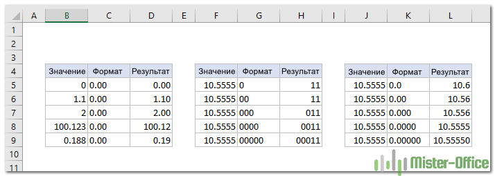
Знак решётки (#) является заполнителем для значащих цифр. Отображает значащие цифры и не отображает лишние нули. Если число состоит из меньшего количества цифр, чем имеется символов # в формате, ничего лишнего не отображается. Например, код #.## будет отображать 1.15 как 1.15 и 1.1 как 1.1.

Знак вопроса (?) Используется для выравнивания цифр. Когда вопросительный знак занимает в числе место, для которого нет значащей цифры, то будет добавлен пробел для визуального выравнивания значений в столбце по десятичной запятой.

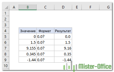
Точка (.) – это десятичная точка в числе. Когда точка используется в пользовательском числовом формате, она будет отображаться всегда, независимо от того, содержит ли число десятичные значения.

Пробел или запятая (,) – это разделитель тысяч в отображаемых цифрах. Его нужно просто включить в код (см.подробнее здесь). Какой именно разделитель нужно использовать (пробел, запятую или что-то другое) – зависит от ваших региональных настроек в панели управления Windows.

А на скриншоте ниже вы видите второй способ применения запятой. Если ее поставить в конце, то значение округляется до тысяч. Соответственно, две запятых – до миллиона.

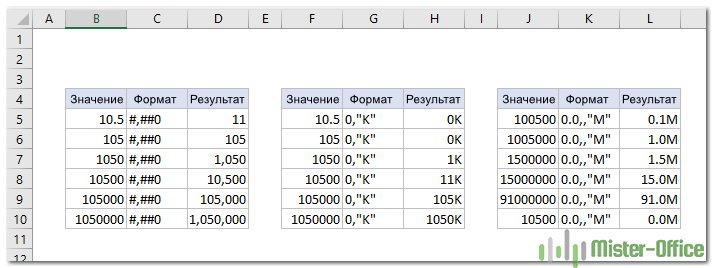
Звездочка (*) используется для повторения символов. Символ, следующий сразу за звездочкой, будет повторяться, чтобы заполнить оставшееся место в ячейке.

Подчеркивание (_) добавляет пробел. Символ, следующий сразу за символом подчеркивания, определяет, сколько места нужно добавить. Обычно символ подчеркивания используется для добавления пробела с целью выравнивания положительных и отрицательных значений, когда числовой формат добавляет круглые скобки только к отрицательным значениям.

Например, конструкция 0_);(0) добавляет немного места справа от положительных чисел, чтобы они оставались выровненными с отрицательными, заключенными в круглые скобки. Подробнее читайте здесь.

Собака (@) – заполнитель для текста. Дает команду, что нужно вывести записанный в ячейке текст. Например, следующий числовой формат будет отображать текстовые значения синим цветом:

0;0;0;[Синий]@

См. ниже дополнительную информацию об использовании цвета.

Посмотрим в действии несколько числовых форматов:

Как вы могли заметить на приведенном выше скриншоте, заполнители цифр ведут себя следующим образом:

Если число, введенное в ячейку, содержит больше цифр справа от десятичной точки, чем имеется заполнителей в формате, то оно «округляется» до такого количества десятичных знаков, сколько есть заполнителей.

Например, если вы введете 12.25 в ячейку с форматом #.# , оно будет отображаться как 12.3.

Все цифры слева от десятичной точки отображаются независимо от количества заполнителей.

Например, если вы введете 252.25 в ячейку с форматом #.# , то будет показано 252.3.

Ниже вы найдете еще несколько примеров, которые, надеюсь, прольют больше света на форматирование чисел в Excel.

Советы и рекомендации по форматированию Excel

Теоретически существует бесконечное количество настраиваемых числовых форматов Excel, которые можно создать с помощью набора знаков, перечисленных в таблице ниже. Следующие советы объясняют наиболее распространенные и полезные их применения.

Код	Описание
Общий	Общий числовой формат
#	Заполнитель цифр, который представляет необязательные цифры и не отображает лишние нули.
0	Заполнитель для цифр, отображающий незначащие нули.
?	Заполнитель цифр, который оставляет место для незначительных нулей, но не отображает их.
.	Десятичная точка
,	Разделитель тысяч. Запятая, следующая за заполнителем цифры, увеличивает значение на тысячу.
%	Умножает на 100 и отображает знак процента.
/	Представляет десятичные числа в виде дробей.
E	Экспоненциальный (научный) вид
[]	Для создания условий

Это так называемые служебные символы, которые определяют, что и как будет показано в ячейке.

Но что, если знак процента или звездочку вы захотите просто показать в ячейке как обычную букву или цифру? Эти знаки не будут отображаться без дополнительной обработки. Например, символы звездочки (*), решетки (#) и процента (%) нельзя использовать непосредственно – они не появятся в ячейке. В качестве дополняющего элемента в этом случае используется обратная косая черта (). Поместив её перед символом, вы можете показывать его в ваших таблицах:

Число	Код	Результат
100	#0	#100
100	*0	*100
100	%0	%100

Еще следует упомянуть специальные символы. Они определяют, как обрабатываются другие символы.

Символ	Что делает	Описание
“”	Выводит любой текст	Позволяет добавлять произвольный текст, заключив его в кавычки.
	Показывает стандартные символы кода	Выводит в ячейке следующий за ним служебный символ, который в обычном виде не отображается.
@	Выводит текст	Показывает текст, введённый в ячейку
_	Пробел	Добавляет один пробел шириной как следующий за ним символ (который не показывается в ячейке). Обычно он используется в сочетании с круглыми скобками для добавления левого и правого отступов, _ ( и _) соответственно.
*	Повтор символа	Повторяет следующий за ним символ, пока ширина ячейки не заполнится. Часто используется в сочетании с пробелом для изменения выравнивания.

Как контролировать количество десятичных знаков

Расположение десятичной точки показано точкой (.). Необходимое количество десятичных знаков определяется нулями (0). Например:

0 или # – отображать ближайшее целое без десятичных знаков.
0.0 или #.0 – 1 знак после запятой.
0.00 или #.00 – 2 десятичных знака и т. д.

Разница между 0 и # при отображении целой части заключается в следующем. Если слева от десятичной точки присутствуют только знаки решетки (#), то числа меньше 1 начинаются с десятичной точки. Например, когда вы введете 0.25 в ячейку с форматом #.00 , число будет выглядеть как .25. Если вы используете 0.00 , то получите 0.25. И вот ещё несколько примеров:

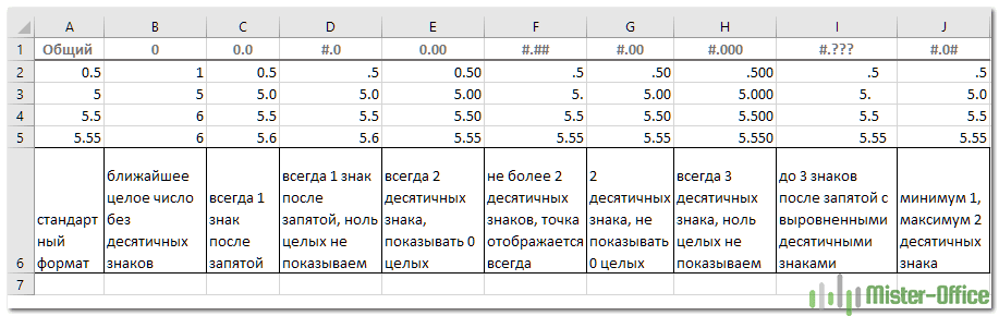
Думаю, эти шаблоны будут вам полезны.

Автоматическое округление

Важно не забывать, что Excel выполняет «визуальное округление» в ячейках.

Если число имеет больше десятичных знаков, чем имеется заполнителей справа от десятичной точки, то оно округляется до количества заполнителей.

Если число содержит больше цифр, чем имеется заполнителей слева от десятичной точки, то отображаются дополнительные разряды. Целая часть не обрезается.

Это только визуальный эффект; фактические значения не изменяются.

Разделитель тысяч

Чтобы создать собственный числовой формат с разделителем тысяч, вставьте пробел в код. Например:

# ### – отображать разделитель тысяч и без десятичных знаков.
# ##0.00 – показать разделитель тысяч и 2 десятичных знака.

Масштабирование до тысяч, миллионов и т. д.

Как показано в предыдущем совете, Microsoft Excel разделяет на разряды тысяч, если используемый разделитель разрядов заключен в любые заполнители цифр – знак решетки (#), вопросительный знак (?) или ноль (0).

Если после разделителя нет никакого заполнителя цифр, то он масштабирует число до тысяч, два последовательных пробела масштабируют в миллионы и так далее.

Например, если формат ячейки «- #.00 » (кавычки здесь только для того, чтобы показать, что есть пробел в конце) и вы вводите в эту ячейку 5000, отображается 5.00.

Использование текста и интервалов.

Если нужно отобразить в ячейке как текст, так и числа, выполните следующие действия:

Чтобы добавить один символ, поставьте перед ним обратную косую черту ().
Добавляя целую текстовую строку, заключите ее в двойные кавычки («»).

Например, чтобы указать, что значения округляются до тысяч и миллионов, вы можете добавить соответственно:

Чтобы отобразить тысячи: #.00 тыс.
Чтобы отобразить миллионы: #.000 » млн»

Совет. Чтобы информацию в ячейке было удобнее читать, добавьте пробел перед текстом.

Ниже для вас несколько примеров:

А вот еще один пример, демонстрирующий, как отображать текст и числа в одной ячейке. Предположим, вы хотите добавить слово «Увеличение» для положительных чисел и «Уменьшение» – для отрицательных. Все, что вам нужно сделать, это включить текст, заключенный в двойные кавычки, в соответствующий раздел кода:

«Увеличение » #.00; «Уменьшение «-#.00; 0

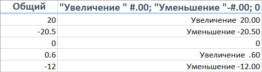
Кроме того, в коды настраиваемого формата Excel можно включать стандартные символы без использования обратной косой черты или кавычек.

Вы можете также использовать здесь и другие специальные символы – такие как валюта, авторское право, товарный знак и т.д. Их можно ввести, набрав четырехзначные коды ANSI, удерживая нажатой клавишу ALT + код ANSI. Вот некоторые из самых полезных:

Условное обозначение	Код	Описание
™	Alt + 0153	Товарный знак
©	Alt + 0169	Символ авторского права
°	Alt + 0176	Символ градусов
±	Alt + 0177	Знак плюс-минус

Например, для отображения температуры вы можете использовать код # «° F» или # «° C». Результат будет выглядеть примерно так:

Вы также можете создать собственный формат Excel, который объединяет определенный текст и текст, записанный в ячейке. Для этого введите дополнительный текст, заключенный в двойные кавычки, в четвёртом разделе кода до или после текстового заполнителя (@), либо с двух его сторон.

Например, чтобы предварить текст, введенный в ячейке, другим текстом, например «Доставлено», можно сделать так:

Символы валюты.

Чтобы создать собственный числовой формат со знаком доллара ($), просто введите его в соответствующий код. Например, в $ #.00 цифра 5 будет отображаться как $5.00 .

Другие символы валюты недоступны на большинстве стандартных клавиатур. Но вы можете ввести популярные валюты таким образом:

Включите NUM LOCK и c цифровой клавиатуры введите код ANSI для символа валюты, который вы хотите отобразить.

Условное обозначение	валюта	Код
€	Евро	ALT + 0128
£	Английский фунт	ALT + 0163
¥	Японская иена	ALT + 0165
¢	Знак цента	ALT + 0162

Набрать символ российского рубля «₽» можно в русской раскладке клавиатуры, нажав правый Alt + 8.

Варианты представления могут выглядеть примерно так:

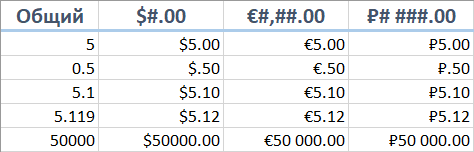
Если вы хотите работать с другой валютой, выполните следующие действия:

Откройте диалоговое окно «Формат ячеек», выберите «Валюта» и укажите нужный вам в раскрывающемся списке «Символ», например, Российский рубль (здесь список валют очень обширный):

Переключитесь в раздел «Все форматы» и измените встроенный формат Excel по своему усмотрению. Или скопируйте код валюты из поля Тип и включите его в свой код.

Как отобразить ведущие нули.

Если вы попытаетесь ввести цифры 005 или 00025 в ячейку с общим форматом по умолчанию, то вы заметите, что Microsoft Excel удаляет ведущие нули, потому что значение 005 совпадает с 5. Но иногда нам нужно именно 005, а не 5!

Самое простое решение — применить к таким ячейкам текстовый формат . Кроме того, вы можете ввести апостроф (‘) перед цифрами. В любом случае Excel поймет, что вы хотите, чтобы любое значение ячейки рассматривалось как текстовая строка. В результате, когда вы вводите 005, все ведущие нули будут сохранены, и ячейка будет отображаться как 005. Но вычисления с таким цифровым значением в виде текста будут невозможны.

Если вы хотите, чтобы все числа в столбце содержали определенное количество цифр с ведущими нулями, создайте собственный формат, включающий только нули.

Как вы помните, в числовом формате Excel ноль – это заполнитель, отображающий незначащие нули. Итак, если вам нужны числа, всегда состоящие из 6 цифр, используйте следующий код: 000000

И теперь, если вы наберете 5 в ячейке, она будет отображаться как 000005; 50 будет отображаться как 000050 и так далее:

Совет. Если вы вводите номера телефонов или какие-то идентификаторы, содержащие начальные нули, то самый простой способ — применить один из предопределенных специальных форматов . Или вы можете создать свой.

Например, чтобы правильно отображать международные семизначные почтовые индексы, используйте этот вариант: 0000000. Для артикулов с ведущими нулями используйте примерно такое: 000-00-0000 .

Проценты

Чтобы отобразить число в виде процента от 100, включите знак процента (%) в код.

Например, чтобы отобразить проценты как целые числа, используйте: #%. В результате 0.25, введенное в ячейку, будет отображаться как 25%.

Для отображения процентов с двумя десятичными знаками: #.00%

Чтобы отобразить проценты с двумя десятичными знаками и разделителем тысяч, используйте этот: # ##.00%

Подробнее о процентном формате читайте в этой статье.

Дроби в числовом формате.

Дроби отличаются тем, что одно и то же число может отображаться разными способами. Например, 1,25 может отображаться как 1 ¼ или 5/4. Тот способ, которым Excel отображает дробь, определяется используемыми кодами формата.

Чтобы десятичные числа отображались как дроби, добавьте косую черту (/) и разделите целую часть пробелом. Например:

# #/# — отображает остаток дроби до 1 цифры.
# ##/## — отображает остаток от дроби до 2 цифр.
# ###/### — отображает остаток дроби до 3 цифр.
###/### — отображает неправильную дробь (дробь, числитель которой больше или равен знаменателю), содержащую до 3 цифр.

Чтобы округлить дроби до определенного знаменателя, укажите его в коде числового формата после косой черты. Например, чтобы отображать десятичные числа как восьмые, используйте следующий формат фиксированнойдроби: # #/8

На следующем скриншоте показаны эти предложения в действии:

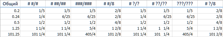
Как вы, наверное, знаете, стандартные форматы дробей Excel выравнивают данные вертикально по линии делителя (/) и отображают целую часть на некотором расстоянии от самой дроби. Чтобы получить такой, используйте заполнители вопросительного знака (?) вместо знаков решетки (#), как показано выше.

Собственный экспоненциальный формат.

Чтобы отображать числа в научном формате, включите заглавную букву E в код. Например:

00E+00 — отображает 1,500,500 как 1,50E+06.
#0.0E+0 — отображает 1,500,500 как 1,5E+6
#E+# — отображает 1,500,500 как 2E+6

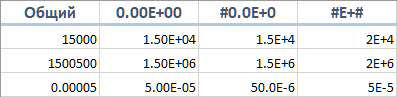
Отрицательные числа в скобках

В начале этого руководства мы обсудили 4 раздела кода, которые составляют числовой формат Excel:

Положительные числа; Отрицательные; Нули; Текст.

Большинство вариантов, которые мы обсуждали до сих пор, содержат только один раздел. Это означает, что он применяется ко всем типам чисел – положительным, отрицательным и к нулям.

Чтобы создать собственное представление для отрицательных значений, вам нужно включить как минимум 2 раздела кода: первый будет использоваться для положительных и нулей, а второй — для отрицательных.

Чтобы показать отрицательные значения в круглых скобках, просто включите их во второй раздел кода, например: #.00; (#.00)

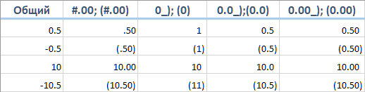
Отображение нулей как тире или пробелов

Встроенный финансовый формат показывает нули как тире. Этот эффект мы также можем легко получить.

Как вы помните, отображение нулевых значений определяется третьим участком кода. Итак, чтобы нули отображались как тире, введите в этом разделе «-». Например:

0.00;(0.00);»-«

Приведенный выше код формата предписывает отображать 2 десятичных разряда для положительных и отрицательных чисел, а также заключать отрицательные в круглые скобки и превращать нули в тире.

Если вам не нужно никакого специального оформления для положительных и отрицательных значений, введите Общий в первом и втором разделах:

Общий; -Общий; «-«

Чтобы превратить нули в пробелы, пропустите третий раздел и введите только конечную точку с запятой:

Общий; — Общий; ; Общий

Добавляем отступы.

Если вы не хотите, чтобы содержимое ячейки подходило вплотную к её границе, вы можете сделать отступ внутри. Чтобы добавить отступ, используйте подчеркивание (_). Это создаст пробел, равный ширине символа, следующего за ним.

Обычно используются следующие коды отступов:

Чтобы сделать отступ от левой границы: _(
Чтобы сделать отступ от правой границы: _)

Чаще всего правый отступ включается в положительный числовой формат, поэтому Excel оставляет место для круглых скобок, заключающих отрицательные числа.

Например, для отступа положительных чисел и нулей справа и текста слева вы можете использовать следующий вариант:

0.00_);(0.00); 0_);_(@

Или вы можете добавить отступы с обеих сторон ячейки:

_(0.00_);_((0.00);_(0_);_(@_)

Коды отступа перемещают данные ячейки на ширину одного символа. Чтобы переместить значения от краев ячейки на большее расстояние, запишите два или более последовательных кода отступа.

На следующем скриншоте вы видите отступ содержимого ячейки на 1 и 2 символа:

Как изменить цвет шрифта.

Изменение цвета шрифта для определенного типа значения — одна из самых простых вещей, которую вы можете сделать с помощью специального числового формата в Excel. Он по умолчанию поддерживает 8 основных цветов.

Чтобы задать цвет для определённого раздела кода формата, введите в этом разделе одно из восьми перечисленных ниже названий цветов в квадратных скобках. Код цвета должен быть в самом начале.

[Черный] [Синий] [Голубой] [Зеленый] [Фиолетовый] [Красный] [Белый] [Желтый]

Например, чтобы оставить общий формат по умолчанию для всех типов значений и изменить только цвет шрифта, используйте код, подобный этому:

[Зеленый]Общий;[Красный]Общий;[Желтый]Общий;[Голубой]Общий

Или комбинируйте цветовые коды с желаемым форматированием чисел. Например, отобразите символ валюты, 2 десятичных знака, разделитель тысяч и покажите нули как тире:

[Синий]# ##0.00₽;[Красный] -# ##0.00₽;[Черный] «-«;[Фиолетовый] @

Результат вы видите на скриншоте.

Цвета по индексу – полезный лайфхак.

Помимо названий цветов, также можно указать цвета по порядковому номеру (Цвет1, Цвет2, Цвет3 и т. Д.). В приведенных ниже примерах используется пользовательский числовой формат: [ЦветX] 0 «▲ ▼», где X — число между 1 и 56:

[ Цвет1 ] 0 «▲ ▼» // черный

[ Цвет2 ] 0 «▲ ▼» // белый

[ Цвет3 ] 0 «▲ ▼» // красный

[ Цвет4 ] 0 «▲ ▼» // зеленый

и т. д.

Символы треугольника были добавлены только для того, чтобы цвета были легче различимы. Скриншот ниже показывает все 56 цветов на стандартном белом фоне. Обратите внимание, что первые 8 показанных цветов соответствуют стандартному списку цветов выше.

Использование символов.

Кроме того, вы можете использовать инструмент «Символ» (вкладка «Главная» или «Вставка»), чтобы найти нужный символ и затем вставить его в ячейку. Из ячейки вы можете скопировать его в буфер обмена и вставить в диалоговое окно «Пользовательский числовой формат».

Совет : Вы также можете вставлять символы, такие как треугольники вверх или вниз. Главное – убедитесь, что они принадлежат к шрифту Arial, а не Wingdings:

Например, в этом случае положительные проценты отображаются треугольником, направленным вверх, а отрицательные значения — треугольником, направленным вниз.

▲ 0,0%; ▼ 0,0%

Символы могут быть весьма эффективными при использовании в отчетах или диаграммах, подобных приведенной ниже:

Повтор символов

Чтобы повторить определенный символ в настраиваемом формате Excel так, чтобы он занимал всю ширину столбца, введите перед ним звездочку (*).

Например, чтобы включить достаточное количество знаков равенства после числа для заполнения ячейки, используйте следующий формат:

#*=

Или вы можете дописать ведущие нули, добавив *0 перед любым числовым форматом, например *0#

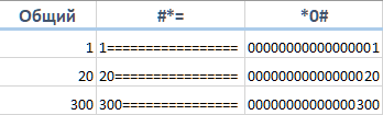
Этот метод обычно используется также для изменения выравнивания ячеек, как показано в следующем совете.

Как изменить выравнивание

Обычный способ изменить выравнивание в Excel — использовать вкладку «Выравнивание» на ленте. Однако при необходимости вы можете «жестко запрограммировать» выравнивание ячеек.

Например, чтобы выровнять цифры слева в ячейке, введите звездочку и пробел после числового кода, например: «#, ### * » (двойные кавычки используются только для того, чтобы показать, что за звездочкой следует пробел, в реальном коде формата они вам не нужны).

Далее вы можете выровнять числа по левому краю, а текстовые записи – по правому краю, используя этот пример:

# ###* ; -# ###* ; 0* ;* @

Этот метод используется во встроенном финансовом формате. Если вы примените его к какой-либо ячейке, затем посмотрите на поле Тип , то вы увидите этот код:

_-* # ##0.00 [$₽-ru-RU]_-;-* # ##0.00 [$₽-ru-RU]_-;_-* «-«?? [$₽-ru-RU]_-;_-@_-

Звездочка, следующая за знаком минус, сообщает Excel, что нужно повторять следующий символ пробела, пока ширина ячейки не будет заполнена. Вот почему финансовый стиль выравнивает минус по левому краю, а само число по правому краю и добавляет между ними столько пробелов, сколько необходимо.

Числовые форматы для текста.

Чтобы отобразить сопроводительный текст вместе с цифровыми данными, заключите его в двойные кавычки («»). Вы можете использовать этот подход для добавления или добавления нужных фраз, как показано в таблице ниже.

Число	Код	Результат
10	0.0 «шт.»	10.0 шт.
5.5	0.0 «литров»	5.5 литров
300	0 «чел.»	300 чел.
95,2	«Оценка:» 0.0	Оценка: 95.2
1 июня	«Дата:» д мммм	Дата: 1 август

Если ваш текст следует после кода числа, то можно обойтись и без кавычек.

Скрыть содержимое ячейки

Фактически вы можете использовать собственный числовой формат, чтобы скрыть все содержимое ячейки.

Код – это просто три точки с запятой и ничего больше ;;;

Чтобы снова отобразить содержимое, вы можете использовать сочетание клавиш CTRL + Shift + ~, которое устанавливает общий формат.

Формат в зависимости от условия

Чтобы пользовательский формат Excel применялся только в том случае, если значение соответствует определенному условию, введите код, состоящий из оператора сравнения и значения, и заключите его в квадратные скобки [].

Например, чтобы отображать числа меньше 100 красным шрифтом, а остальные числа – зеленым, используйте следующий код:

[Красный][<100];[Зеленый][>=100]

Кроме того, вы можете указать желаемый числовой формат, например, показать 2 десятичных знака:

[Красный][<100]0.00;[Зеленый][>=100]0.00

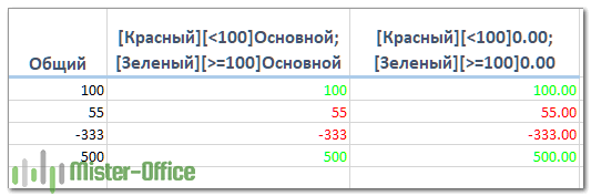
А вот еще один чрезвычайно полезный, хотя и редко используемый совет по форматированию. Если в ячейке отображаются как числа, так и текст, вы можете создать условный формат, чтобы отображать разное содержание в зависимости от числа. Например:

[>=1000]#.000′ » т» ;#.0##» кг»

Это работает следующим образом:

Если значение ячейки меньше 1000, значение будет отображаться как «килограммы».
Если значение ячейки больше 1000, то значение автоматически округлится до тысяч с тремя знаками после запятой. И единица измерения теперь уже будет «тонна».

Продолжая пример, вы можете отображать обычные дроби вместо десятичных:

[<1]?.???;# ?/?

Числа меньше 1 отображаются в виде десятичной дроби, а остальные – в виде обычной.

Примеры вы видите на скриншоте.

Форматы даты и времени в Excel

Форматы даты и времени Excel — очень специфический случай, и у них есть свои правила. Для получения подробной информации и примеров, пожалуйста, ознакомьтесь со следующими руководствами:

Как создать собственный формат даты в Excel
Как создать собственный формат времени в Excel

Наконец, вот несколько советов по быстрому применению ваших пользовательских форматов к другим ячейкам и книгам:

Пользовательский формат Excel хранится в книге, в которой он создан, и недоступен ни в одной другой книге. Чтобы использовать его постоянно, вы можете сохранить текущий файл как шаблон, а затем использовать его как основу для новой книги.
Чтобы применить настраиваемый формат к другим ячейкам одним щелчком мыши, сохраните его как стиль Excel. Для этого просто выберите любую ячейку с подходящим оформлением, перейдите на вкладку «Главная» в группу «Стили» и нажмите «Новый стиль ячейки…». Читайте подробную инструкцию по этой ссылке.

Итак, вот как вы можете изменить формат чисел в Excel и создать собственное их представление.

Благодарю вас за чтение и надеюсь увидеть вас снова!

Формат времени в Excel — Вы узнаете об особенностях формата времени Excel, как записать его в часах, минутах или секундах, как перевести в число или текст, а также о том, как добавить время с помощью…

7 способов поменять формат ячеек в Excel — Мы рассмотрим, какие форматы данных используются в Excel. Кроме того, расскажем, как можно быстро изменять внешний вид ячеек самыми различными способами. Когда дело доходит до форматирования ячеек в Excel, большинство…

Как удалить формат ячеек в Excel — В этом коротком руководстве показано несколько быстрых способов очистки форматирования в Excel и объясняется, как удалить форматы в выбранных ячейках. Самый очевидный способ сделать часть информации более заметной — это…

8 способов разделить ячейку Excel на две или несколько — Как разделить ячейку в Excel? С помощью функции «Текст по столбцам», мгновенного заполнения, формул или вставив в нее фигуру. В этом руководстве описаны все варианты, которые помогут вам выбрать технику, наиболее подходящую…

Источник

How to Custom Format Numbers in Excel

Excel custom number formatting is nothing but making the data look better or visually appealing. Excel has many inbuilt number formatting. On top of this, we can customize the Excel number formatting by changing the format of the numbers.

Excel works on numbers and is based on the format we give. It shows the result. For example, look at the below example.

In cell C1, we have the number 43473.

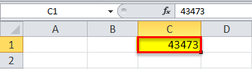
As of now, the Excel format of the custom number is “General.”

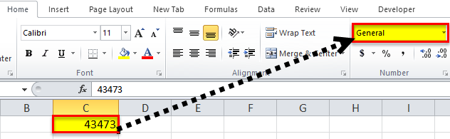
If we click on the drop-down list, there are several built-in number formats available here, like “Number,” “Currency,” “Accounting,” “Date,” “Short Date,” “Time,” “Percentage,” and many more.

These are all already predefined formatting, but we can customize all these and make the alternative number formatting, and this is called “Custom Number Formatting.”

How to Custom Format Numbers in Excel
- How to Create a Custom Number Format in Excel? (Using Shortcut Key)
  - #1 – Date Custom Format
  - #2 – Time Custom Format
  - #3 – Number Custom Format
  - #4 – Show Thousand numbers in K, M, and B Format
  - #5 – Show Negative Numbers in Brackets & Positive Numbers with + Sign
  - #6 – Show Numbers Hide text Values
  - #7 – Show Numbers With Conditional Colors
- Things to Remember
- Recommended Articles

How to Create a Custom Number Format in Excel? (Using Shortcut Key)

Normal formatting is available under the Home tab. We need to right-click on the specific cell and select “Format Cells” to do the custom formatting.

You can download this Custom Number Format Excel Template here – Custom Number Format Excel Template

The shortcut key to formatting is Ctrl + 1.

Ok, now we will discuss the different types of formattings.

#1 – Date Custom Format

It is the most common formatting we work with day in and day out. Now, look at the below image. We have a number in cell C1.

We want to show this number as a date. So, we must select the cell and press Ctrl + 1.

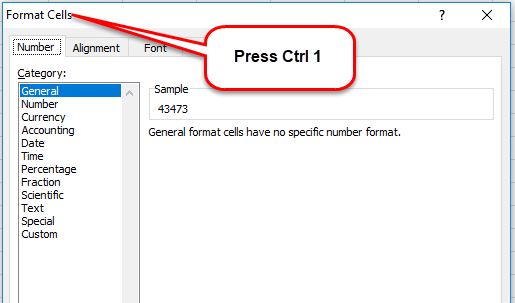
Next, we must select the “Custom” format in Excel and type the required date format under the “Type:” section.

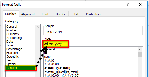
DD means the date should be first and two digits.
MM means the month should be second and two digits.
YYYY means the year should be last and four digits.

Now, press the “Enter” key. It will show the date in the mentioned format.

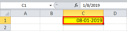
Below are some of the important date format codes.

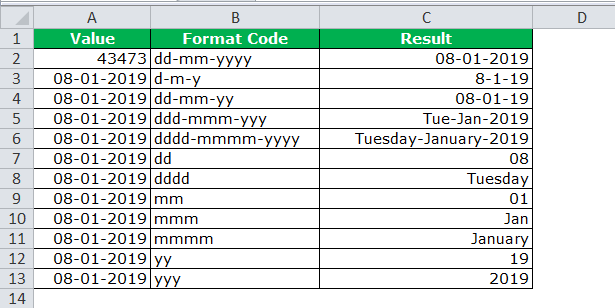
#2 – Time Custom Format

We can customize the format of the time as well. Below are the codes for the time format.

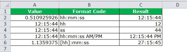
If you observe the above table, we have not mentioned the code to show the minute. Unfortunately, we cannot show only the minute section since “m” & “mm” coincide with the month.

In the case of time exceeding more than 24 hours, we need to mention the hours in brackets, i.e. [hh]

#3 – Number Custom Format

When we are working with numbers, it is very important how we show the numbers to the readers. There are several ways we can show up the numbers; the codes below will help you design your number format.

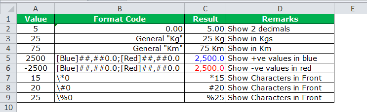
#4 – Show Thousand numbers in K, M, and B Format

Showing numbers in lakhs can sometimes require a lot of cell space and not fit in the report, but we can customize the number format in Excel.

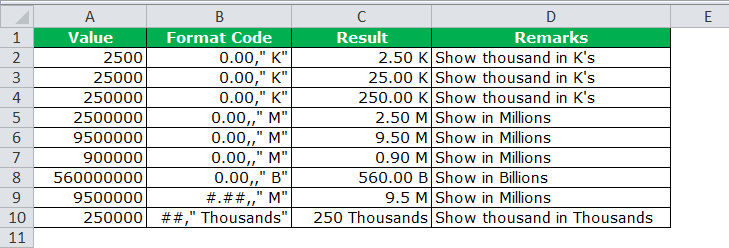
#5 – Show Negative Numbers in Brackets & Positive Numbers with + Sign

Showing negative numbers in brackets and positive numbers with the + sign will make the number look beautiful.

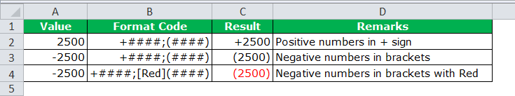
#6 – Show Numbers Hide text Values

Sometimes, showing only numerical values and hiding all the text values technique is required. So the below code can help us with this.

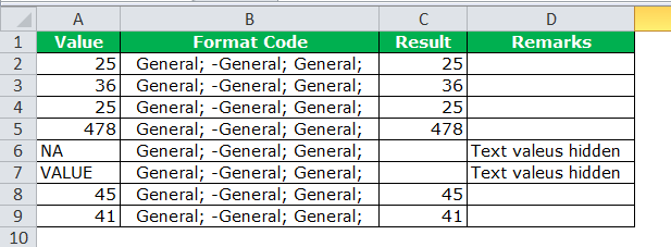
#7 – Show Numbers With Conditional Colors

We have seen cases where we wanted to show some values in “blue” and some in “green.” By changing the number format, we can alter the font colors.

Things to Remember

These are the most commonly used number formats, but several are available.
Displaying huge numbers with millions and billions will make the report more appealing. Nobody wants to count the zeros and read. Rather, they like millions and billions in front of the numbers.
We can show the different numbers in different colors.

Create a custom format code

Format code guidelines

See also

Need more help?

Want more options?

Introduction

What can you do with custom number formats?

Where can you use custom number formats?

What is a number format?

Where can you find number formats?

General is default

How to change number formats

Shortcuts for number formats

Where to enter custom formats

How to create a custom number format

How to edit a custom number format

Structure and Reference

Not all sections required

Characters that display natively

Escaping characters

Placeholders

Automatic rounding

Number formats for TEXT

Number formats for DATES

Number formats for TIME

Number formats for ELAPSED TIME

Number formats for COLORS

Colors by index

Apply number formats in a formula

Measurements

Conditionals

Plural text labels

Telephone numbers

Hide all content

Other resources

How to create a custom number format in Excel

Basics

Syntax

Placeholders and the Cheat Sheet

Common Practices

Display and control of the first digit and decimals

Add text to numbers

Hide value

Replace zeroes with dashes

Start with zeroes

Dealing with thousands, millions, and more

Display numbers as phone numbers

Showing Month and Weekday Names

Come in Colors Everywhere

Conditions

How to Create a Custom Number Format

Number Format Codes

Special Characters in Number Formats

Custom Number Format Examples

Custom Number Format for Thousands and Millions

Display Leading Zeros and Include Commas

Display Units Without Converting to Text

Special Time Formats

Including Special Symbols

Displaying Fractions

Trailing and Leading Characters to Fill a Cell

Custom Number Formats for Chart Axes and Labels

Other Tricks

Custom Number Format Color Codes

Conditional Operators

Custom Location Codes for Dates

Other Notes About Custom Number Formats

References

How do I show column numbers in Excel?

How do I convert text to values in Excel?

How do I convert a column of numbers to column names in Excel?

How do I change the number format in Excel?

Why does Excel have numbers for columns?

How do I show columns and row numbers in Excel?

How do I get columns and row numbers in Excel?

How do I get row numbers in Excel?

How do I format numbers in Excel?

What are the different ways in formatting numbers?

How do I change the column title in Excel?

How do I change rows and column names in Excel?