
In a Data Model, each column has an associated data type that specifies the type of data the column can hold: whole numbers, decimal numbers, text, monetary data, dates and times, and so on. Data type also determines what kinds of operations you can do on the column, and how much memory it takes to store the values in the column.
If you’re using the Power Pivot add-in, you can change a column’s data type. You might need to do this if a date column was imported as a string, but you need it to be something else. For more information, see Set the data type of a column in Power Pivot.
In this article
-
Summary of data types
-
Table Data Type
-
-
Implicit and explicit data type conversion in DAX formulas
-
Table of Implicit Data Conversions
-
Addition (+)
-
Subtraction (-)
-
Multiplication (*)
-
Division (/)
-
Comparison operators
-
-
-
Handling blanks, empty strings, and zero values
Summary of data types
The following table lists data types supported in a Data Model. When you import data or use a value in a formula, even if the original data source contains a different data type, the data is converted to one of these data types. Values that result from formulas also use these data types.
|
Data type in Excel |
Data type in DAX |
Description |
|---|---|---|
|
Whole Number |
A 64 bit (eight-bytes) integer value 1, 2 |
Numbers that have no decimal places. Integers can be positive or negative numbers, but must be whole numbers between -9,223,372,036,854,775,808 (-2^63) and 9,223,372,036,854,775,807 (2^63-1). |
|
Decimal Number |
A 64 bit (eight-bytes) real number 1, 2 |
Real numbers are numbers that can have decimal places. Real numbers cover a wide range of values: Negative values from -1.79E +308 through -2.23E -308 Zero Positive values from 2.23E -308 through 1.79E + 308 However, the number of significant digits is limited to 15 decimal digits. |
|
TRUE/FALSE |
Boolean |
Either a True or False value. |
|
Text |
String |
A Unicode character data string. Can be strings, numbers or dates represented in a text format. Maximum string length is 268,435,456 Unicode characters (256 mega characters) or 536,870,912 bytes. |
|
Date |
Date/time |
Dates and times in an accepted date-time representation. Valid dates are all dates after January 1, 1900. |
|
Currency |
Currency |
Currency data type allows values between -922,337,203,685,477.5808 to 922,337,203,685,477.5807 with four decimal digits of fixed precision. |
|
N/A |
Blank |
A blank is a data type in DAX that represents and replaces SQL nulls. You can create a blank by using the BLANK function, and test for blanks by using the logical function, ISBLANK. |
1 DAX formulas do not support data types smaller than those listed in the table.
2 If you try to import data that has very large numeric values, import might fail with the following error:
In-memory database error: The ‘<column name>’ column of the ‘<table name>’ table contains a value, ‘1.7976931348623157e+308’, which is not supported. The operation has been cancelled.
This error occurs because Power Pivot uses that value to represent nulls. The values in the following list are synonyms for the null value:
|
Value |
|
|---|---|
|
9223372036854775807 |
|
|
-9223372036854775808 |
|
|
1.7976931348623158e+308 |
|
|
2.2250738585072014e-308 |
Remove the value from your data and try importing again.
Table Data Type
DAX uses a table data type in many functions, such as aggregations and time intelligence calculations. Some functions require a reference to a table; other functions return a table that can then be used as input to other functions. In some functions that require a table as input, you can specify an expression that evaluates to a table; for some functions, a reference to a base table is required. For information about the requirements of specific functions, see DAX Function Reference.
Implicit and explicit data type conversion in DAX formulas
Each DAX function has specific requirements as to the types of data that are used as inputs and outputs. For example, some functions require integers for some arguments and dates for others; other functions require text or tables.
If the data in the column you specify as an argument is incompatible with the data type required by the function, DAX in many cases will return an error. However, wherever possible DAX will attempt to implicitly convert the data to the required data type. For example:
-
You can type a date as a string, and DAX will parse the string and attempt to cast it as one of the Windows date and time formats.
-
You can add TRUE + 1 and get the result 2, because TRUE is implicitly converted to the number 1 and the operation 1+1 is performed.
-
If you add values in two columns, and one value happens to be represented as text («12») and the other as a number (12), DAX implicitly converts the string to a number and then does the addition for a numeric result. The following expression returns 44: = «22» + 22
-
If you attempt to concatenate two numbers, Excel will present them as strings and then concatenate. The following expression returns «1234»: = 12 & 34
The following table summarizes the implicit data type conversions that are performed in formulas. Excel performs implicit conversions whenever possible, as required by the specified operation.
Table of Implicit Data Conversions
The type of conversion that is performed is determined by the operator, which casts the values it requires before performing the requested operation. These tables list the operators, and indicate the conversion that is performed on each data type in the column when it is paired with the data type in the intersecting row.
Note: Text data types are not included in these tables. When a number is represented as in a text format, in some cases Power Pivot will attempt to determine the number type and represent it as a number.
Addition (+)
|
Operator (+) |
INTEGER |
CURRENCY |
REAL |
Date/time |
|---|---|---|---|---|
|
INTEGER |
INTEGER |
CURRENCY |
REAL |
Date/time |
|
CURRENCY |
CURRENCY |
CURRENCY |
REAL |
Date/time |
|
REAL |
REAL |
REAL |
REAL |
Date/time |
|
Date/time |
Date/time |
Date/time |
Date/time |
Date/time |
For example, if a real number is used in an addition operation in combination with currency data, both values are converted to REAL, and the result is returned as REAL.
Subtraction (-)
In the following table the row header is the minuend (left side) and the column header is the subtrahend (right side).
|
Operator (-) |
INTEGER |
CURRENCY |
REAL |
Date/time |
|---|---|---|---|---|
|
INTEGER |
INTEGER |
CURRENCY |
REAL |
REAL |
|
CURRENCY |
CURRENCY |
CURRENCY |
REAL |
REAL |
|
REAL |
REAL |
REAL |
REAL |
REAL |
|
Date/time |
Date/time |
Date/time |
Date/time |
Date/time |
For example, if a date is used in a subtraction operation with any other data type, both values are converted to dates, and the return value is also a date.
Note: Data models also supports the unary operator, — (negative), but this operator does not change the data type of the operand.
Multiplication (*)
|
Operator (*) |
INTEGER |
CURRENCY |
REAL |
Date/time |
|---|---|---|---|---|
|
INTEGER |
INTEGER |
CURRENCY |
REAL |
INTEGER |
|
CURRENCY |
CURRENCY |
REAL |
CURRENCY |
CURRENCY |
|
REAL |
REAL |
CURRENCY |
REAL |
REAL |
For example, if an integer is combined with a real number in a multiplication operation, both numbers are converted to real numbers, and the return value is also REAL.
Division (/)
In the following table the row header is the numerator and the column header is the denominator.
|
Operator (/) (Row/Column) |
INTEGER |
CURRENCY |
REAL |
Date/time |
|---|---|---|---|---|
|
INTEGER |
REAL |
CURRENCY |
REAL |
REAL |
|
CURRENCY |
CURRENCY |
REAL |
CURRENCY |
REAL |
|
REAL |
REAL |
REAL |
REAL |
REAL |
|
Date/time |
REAL |
REAL |
REAL |
REAL |
For example, if an integer is combined with a currency value in a division operation, both values are converted to real numbers, and the result is also a real number.
Comparison operators
In comparison expressions Boolean values are considered greater than string values and string values are considered greater than numeric or date/time values; numbers and date/time values are considered to have the same rank. No implicit conversions are performed for Boolean or string values; BLANK or a blank value is converted to 0/»»/false depending on the data type of the other compared value.
The following DAX expressions illustrate this behavior:
=IF(FALSE()>»true»,»Expression is true», «Expression is false»), returns «Expression is true»
=IF(«12″>12,»Expression is true», «Expression is false»), returns «Expression is true».
=IF(«12″=12,»Expression is true», «Expression is false»), returns «Expression is false»
Conversions are performed implicitly for numeric or date/time types as described in the following table:
|
Comparison Operator |
INTEGER |
CURRENCY |
REAL |
Date/time |
|---|---|---|---|---|
|
INTEGER |
INTEGER |
CURRENCY |
REAL |
REAL |
|
CURRENCY |
CURRENCY |
CURRENCY |
REAL |
REAL |
|
REAL |
REAL |
REAL |
REAL |
REAL |
|
Date/time |
REAL |
REAL |
REAL |
Date/time |
Top of Page
Handling blanks, empty strings, and zero values
In DAX, a null, blank value, empty cell, or a missing value are all represented by the same new value type, a BLANK. You can also generate blanks by using the BLANK function, or test for blanks by using the ISBLANK function.
How blanks are handled in operations, such as addition or concatenation, depends on the individual function. The following table summarizes the differences between DAX and Microsoft Excel formulas, in the way that blanks are handled.
|
Expression |
DAX |
Excel |
|---|---|---|
|
BLANK + BLANK |
BLANK |
0 (zero) |
|
BLANK +5 |
5 |
5 |
|
BLANK * 5 |
BLANK |
0 (zero) |
|
5/BLANK |
Infinity |
Error |
|
0/BLANK |
NaN |
Error |
|
BLANK/BLANK |
BLANK |
Error |
|
FALSE OR BLANK |
FALSE |
FALSE |
|
FALSE AND BLANK |
FALSE |
FALSE |
|
TRUE OR BLANK |
TRUE |
TRUE |
|
TRUE AND BLANK |
FALSE |
TRUE |
|
BLANK OR BLANK |
BLANK |
Error |
|
BLANK AND BLANK |
BLANK |
Error |
For details on how a particular function or operator handles blanks, see the individual topics for each DAX function, in the section, DAX Function Reference.
Top of Page
Since the start of Excel, one cell could only contain one piece of data.
With Excel’s new rich data type feature, this is no longer the case. We now have multiple data fields inside one cell!
When you think of data types you might be thinking about text, numbers, dates or Boolean values, but these new data types are quite different. They are really connections to an online data source that provides more information about the data.
At present there are two data types available in Excel; Stocks and Geography.
For example, with the new stock data type our cell might display the name of a company, but will also contain information like the current share price, trading volume, market capitalization, employee head count, and year of incorporation for that company.
The connections to the additional data are live, which is especially relevant for the stock data. Since data like the share price is constantly changing, you can always get the latest data by refreshing the connection.
Caution: The stock data is provided by a third party. Data is delayed, and the delay depends on which stock exchange the data is from. Information about the level of delay for each stock exchange can be found here.
The data connection for the geography data type is also live and can be refreshed, but these values should change very infrequently.
Video Tutorial
Converting Text To Rich Data Types
Whichever data type you want to use, converting cells into a data type is the same process. As you might expect, the new data types have been placed in the Data tab of the Excel ribbon in a section called Data Types.
At present the two available data types fit nicely into the space. But you can click on the lower right area to expand this space, which seems to suggest more data types are on their way!
You will need to select the range of cells with your text data and go to the Data tab and click on either the Stock or Geography data type. This will convert the plain text into a rich data type.
Warning: You can’t convert cells containing formula to data types.
You can easily tell when a cell contains a data type as there will be a small icon on the left inside the cell. The Federal Hall icon indicates a Stock data type and the map icon indicates a Geography data type.
Right Click Data Type Menu
The right click menu has a contextual option which is only available when the right click is performed on a cell or range containing data types. This is where you’ll find most commands related to data types.
Automatic Data Type Conversion
If you want to add to your list of data type cells, all you need to do is type in the cell directly below a data type and Excel will automatically convert it to the same data type as above.
Correcting Missing Data Types
Excel will try and convert your text with the best match, but it might not always find a suitable match or there might be some ambiguity. When this happens, a question mark icon will appear in the cell. You can click on this icon to help Excel find the best match.
Click on the question mark icon and this will open the Data Selector window pane. You can use the search bar to try and locate the desired result and then click on the Select button to accept one of the options presented.
Changing Data Types
In case Excel made the wrong choice, you can also change a data type. You right click on the data and choose Data Type then Change from the menu. This will also open the Data Selector window pane.
Currency & Cryptocurrency Data
With the stock data type, you can get more than just stocks from a company name. The stock data type can also be used for currency and cryptocurrency conversions.
Currency Exchange Rate Pairs
You can convert pairs of currencies into data types to get exchange rates.
Cryptocurrency Exchange Rate Pairs
You can convert cryptocurrency/currency pairs into data types too. Exchange rates between cryptocurrencies are currently not supported.
Country, State, Province, County & City Data
The geography data type supports most types of geographies. Countries, states, provinces, counties and cities will all work.
The fields available for each type of geography will vary. For example, a country, state, province, or county might have a capital city field, but this field will not be available for a city.
Data Cards
There is a pretty cool way to view the data contained inside a cell that’s been. When you click on the icon for any data type a Data Card will appear.
This is also accessible through the rick click menu. Right click then choose Data Type from the menu then choose Data Card.
Data cards will show all the available data for that cell and may also include a picture related to the data such as a company logo or a country’s flag.
Each piece of data displayed in the card also comes with an Extract to grid button that becomes visible when you hover the mouse cursor over that area. This will extract the data into the next blank cell to the right of the data type.
In the lower right corner of the card, there’s a flag icon. This allows you to report any bad data that might be displayed in the card back to Microsoft.
Extracting Data
The data cards are nice for viewing the data inside a cell, but how can you use this data? There are Extract to grid buttons for each piece of data inside the data cards, but these will only extract data for one cell. What if you want to extract data from many cells?
When you select a range of cells containing data types, an Extract to grid icon will appear at the top right of the selected range. When you click on this, Excel will show a list of all the available data that can be extracted. Unfortunately, you’ll only be able to select one piece of data at a time.
A handy feature with extracting data, is that Excel takes care of the number formatting. Whether you’re extracting a percent, number, currency, date or time, Excel will apply the relevant formatting.
Dot Formulas & FIELDVALUE Function
Extract is probably not the best word to use for the Extract to grid button. If you check the contents of the extracted data, you’ll see it’s a formula reference to the data type cell.
Dot Formula Notation
In fact, you don’t need to use the extract to grid button to create these formulas. You can write them just like any other Excel formula.
= B3.PopulationThe above formula will return the population of Canada.
= B3.Population / B3.AreaThe above formula will give us a density calculation and return 3.7 people per square kilometer.
Thankfully, Excel’s formula IntelliSense will show you all the available fields when you create a cell reference to a data type cell followed by a period. This makes writing data type formulas easy!
Note: When the field name contains spaces, the field reference needs to be encased with square braces.
Formulas only support one dot.
= B3.CapitalThe above formula will return the capital of Canada, which is geographical data.
= B3.Capital.PopulationBut the above formula won’t return the population of the capital city of Canada. To get this information, you would need to extract the capital, then copy and paste the result as a value, then convert that value to a data type, then extract the population.
FIELDVALUE Function
The FIELDVALUE function was introduced with data types and can be used to get the exact same results from a data type cell.
= FIELDVALUE(Value, Field)This new function has two arguments:
- Value is a reference to a data type.
- Field is the name of a field in the data type.
Warning: The FIELDVALUE function does not have IntelliSense for the available fields in a data type.
= FIELDVALUE(B3, "Population")The previous example to return the population of Canada can be written as above using the FIELDVALUE function.
= FIELDVALUE(B3, "Population") / FIELDVALUE(B3, "Area")The previous example to return the population density can be written as above using the FIELDVALUE function.
New FIELD Error Type
A new #FIELD! error has been added to Excel for the dot formulas and FIELDVALUE function. This error can be returned for several reasons.
- The field does not exist for the data type.
- The value referenced in the formula is not a data type.
- The data does not exist in the online service for the combination of value and field.
In the above example, Ireland is returning a #FIELD! error for the abbreviation because this data is missing online.
Refreshing Data
How do you refresh data? Using the Refresh and Refresh All commands found in the Data tab will refresh any data types you have in your spreadsheet.
This means you can use the keyboard shortcuts Alt + F5 (refresh) and Ctrl + Alt + F5 (refresh all) to refresh data types.
Using the Refresh command will refresh all cells in the workbook that are the same data type as your active cell.
The Refresh All command will refresh all cells of any data type.
Warning: Refresh All will also refresh all other connections in the workbook such as pivot tables and power queries.
There is also a refresh method that is proprietary to data types. If you select a cell with a data type, you can right click and choose Data Type from the menu then choose Refresh. This will refresh all cells in the workbook that are the same data type as the selected cell and won’t refresh any other connections like pivot tables or power query.
Unlinking Data
If you no longer want your data connected, you can unlink the data by converting it back to regular text. The only way to do this is to right click on the selected range of data then choose Data Type from the menu and select Change to Text.
Warning: Linking and unlinking data might change your data.
When you convert text to a data type and then convert it back to text, you might not get your original text back exactly as it was. It’s best to create a copy of any text data before converting to a data type so you always have the original text.
Using Tables With Data Types
You don’t need to use Excel tables with data types, but there is a nice bonus feature with tables when extracting data. Excel will create the column headings for you.
Note: You can create an Excel table from the Insert tab with the Table command or using the keyboard shortcut Ctrl + T.
Learn more about Excel tables: Everything You Need to Know About Excel Tables
The Extract to grid button will appear anytime the active cell is inside a table containing data types. The active cell does not need to be on a cell containing a data type.
When there are two or more columns with data type inside a table, the Extract to grid button will be based on the right most column. Unfortunately, this means you can’t extract from any other columns.
Using Sort & Filter With Data Types
Sorting and filtering data types has a nice feature that allows you to sort and filter based on any field even if it hasn’t been extracted.
Note: Turn on the sort and filter toggles for any table or list by using the Ctrl + Shift + L keyboard shortcut.
When you click on the sort and filter toggle of a column of data types, you will be able to select a field from a drop down at the top of the menu. This will change the field which sorting and filtering is based on.
For example, we could select the Year incorporated field and sort our list of companies from oldest to newest, or filter out any company incorporated after the year 2000.
Finding Data Types In A Workbook
Data types are visually distinct because of the icons in cell, so distinguishing between a regular cell and a data type cell is easy. But what if you want to locate all the data type cells in a large workbook? Visual inspection might not be practical.
Since data types are not supported by earlier versions of Excel, the easiest way to locate them in a workbook is with Excel’s check compatibility feature.
Note: Check compatibility can be found in the File tab ➜ Info ➜ Check for Issues ➜ Check Compatibility.
The compatibility checker will list out all the features in the workbook that are not backwards compatible with prior version of Excel. To find any data types, you can look for the words “This workbook contains data types…” in the summary. Each summary will also have a Find hyperlink that will take you to the location and select those cells.
Note: Selecting only Excel 2016 from the Select versions to show button will reduce the results in the compatibility checker and make finding the data types easier.
Conclusions
With rich Data Types you can now get more from your data without leaving Excel to use your favourite search engine.
You can quickly and easily get current financial data, currency rates, cryptocurrency values and geographical data with a couple clicks.
This is a very powerful feature in Excel you need to start using, and with the hint of more data types to come, will become even more useful.
About the Author
John is a Microsoft MVP and qualified actuary with over 15 years of experience. He has worked in a variety of industries, including insurance, ad tech, and most recently Power Platform consulting. He is a keen problem solver and has a passion for using technology to make businesses more efficient.
Asked
10 years, 1 month ago
Viewed
13k times
Is there any way in which I can predefine data type of a column of an excel sheet ?
For eg. when I enter 0022598741 in a column it will be formatted as 22598741 but I want it as it is.In this case this particular column takes the data as number type but I want it to be taken as text type.
- excel
asked Feb 19, 2013 at 14:19
![]()
SharmiSharmi
791 gold badge1 silver badge10 bronze badges
2
-
As this question stands, it will be a better fit over on SuperUser.
Feb 19, 2013 at 14:22
-
@Buggabill already flagged to move.
Feb 19, 2013 at 14:22
1 Answer
Format it as Text before input: right click > cell properties.
answered Feb 19, 2013 at 14:22
![]()
Peter L.Peter L.
7,2465 gold badges34 silver badges53 bronze badges
2
-
Actually I need to predefine the column type before hand and then it will be downloaded somewhere else and used. So will «right click > cell properties» work in that case ?
Feb 19, 2013 at 14:26
-
For sure and that’s the best way to preserve input: select entire column, format as text, save the file and send wherever you need -format will be kept.
Feb 19, 2013 at 14:27
- The Overflow Blog
- Featured on Meta
Related
Hot Network Questions
-
Why does GM Larry claim that this sacrifice is brilliant?
-
Add a CR before every LF
-
MOSFET Overheating, Arduino heating pad project
-
What is the difference between elementary and non-elementary proofs of the Prime Number Theorem?
-
How do I create BLeeM’s «Emphasis Rolls» on Anydice?
-
Reference request for condensed math
-
Etiquette (and common sense) rules for MTB cyclists
-
For the purposes of the Regenerate spell, does a snail shell count as a limb?
-
Why are accessible states taken as eigenstates in statistical physics? Is the resolution via decoherence?
-
Open + Barre Chord Combinations
-
Looking for a 90’s sorcery game on Atari ST
-
Parse a CSV file
-
What does the Honorable Chairman mean?
-
Is there a way to sign a transaction?
-
Deal or No Deal, Puzzling Edition
-
If I overpay estimated taxes in Q1, am I allowed to underpay in the other quarters?
-
Hours at work rounded down
-
Does Ohm’s law always apply at any instantaneous point in time?
-
Documenting footers in concrete slab for future patio cover
-
Why is knowledge inside one’s head considered privileged information but knowledge written on a piece of paper is not?
-
Can I apply for ESTA with passport valid since february?
-
What kind of fallacy is it to say if abolition of something isn’t possible, we shouldn’t attempt to address it at all?
-
Inconsistent kerning in units when using detect-all
-
Good / recommended way to archive fastq and bam files?
more hot questions
Question feed
Your privacy
By clicking “Accept all cookies”, you agree Stack Exchange can store cookies on your device and disclose information in accordance with our Cookie Policy.
AI powered Excel Data Types will transform the way we work with Excel by enabling a cell to contain much more than text, numbers or formulas.
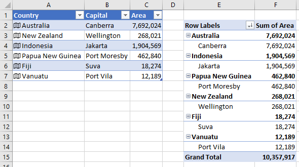
There are currently two Excel data types available to Office 365 users*; Stocks and Geography. Let’s start with the Geography Data Type that can take a table of countries and return rich data that can be referenced in Excel formulas and expand into further columns.
* The new data types are starting to roll out to Office 365 subscribers over the coming weeks and months.
Note: Excel Data Types require an internet connection.
Taking the example above, we can also view the underlying data for a single country by left-clicking on the geography icon in the cell to the left of the country name. This brings up the card with the data available for that country, as shown below. The scroll bar reveals the different information available and if I want to add it to my table I simply click the ‘Extract’ icon in the card.
![]()
When we add fields to our table using the methods shown above, we aren’t adding hard coded text. If you look at the formula bar (below), you’ll see it’s a formula that references the Table Country column [@Country] followed by the dot “.” operator and then the field name ‘Capital’:
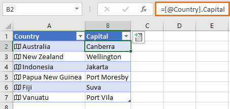
Note: the formula in cell B2 above uses the Excel Table Structured reference, [@Country]. The [@Country] could be replaced with the cell reference, A2. i.e. the formula could also be written: =A2.Capital
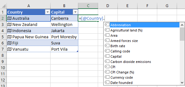
We can therefore add fields by referencing one of the geography cells followed by the dot operator to bring up a list of available fields:
You can use these references in any function as they are full, calculation enabled, first class data types in cells.
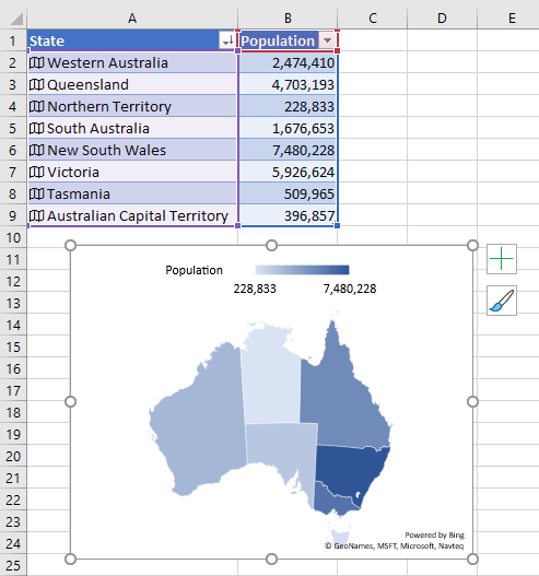
They can also support charts:
Or PivotTables:
Note: You cannot load Data Types into Power Query (yet) as it will generate an error on the column containing the Data Type icon.
Sort and Filter Excel Data Types
When you filter a column containing data types you have a new option that allows you to choose which field you want to sort or filter by, as you can see in the orange box in the image below:
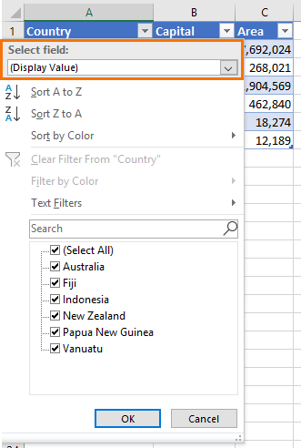
If I select ‘GDP’ from the field list drop down, you’ll notice the sort and filter options reflect the GDP field:
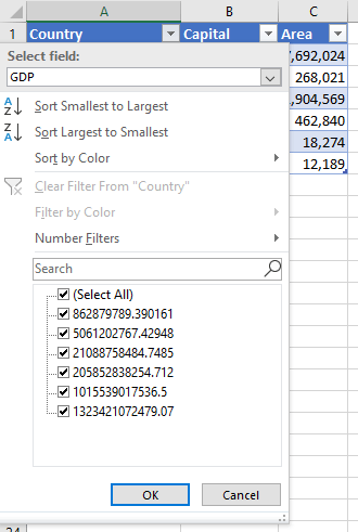
Effectively sorting or filtering on a field not even present in the table itself. Wow!
That said, you can’t tell what field the data is sorted on once it has been applied. However, if you Filter on another field it will be retained in the filter drop down when you revisit it. I’ve reported this to Microsoft in the hope that they retain the selected sort field information in a future update.
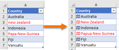
Messy Data
Excel is good at correcting spelling errors and incorrect capitalisation with intelligent conversions. For example, the before (left) and after (right) images below show New Zealand and Papua New Guinea are corrected after the Data Type is applied:
Resolving Ambiguity in Excel Data Types
Sometimes there can be ambiguity when Excel tries to identify locations or stock codes that are present in multiple locations or multiple exchanges.
For example, the abbreviations for states in Australia are often found elsewhere. If I try to convert the table below to geography data types:
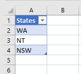
I get the result shown below where it finds New South Wales, but it’s not sure about WA and NT. For these locations Excel opens the ‘Data Selector’ pane and offers some suggested results. However, I want Western Australia for WA and it’s not listed.
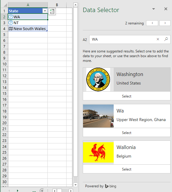
In this case I can type in the full name of the state in the search box and then click the ‘Select’ button to insert it to my table:
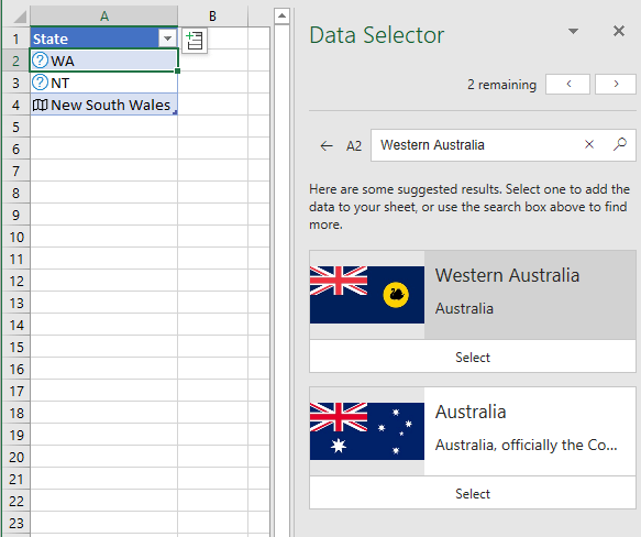
And repeat for Northern Territory (NT).
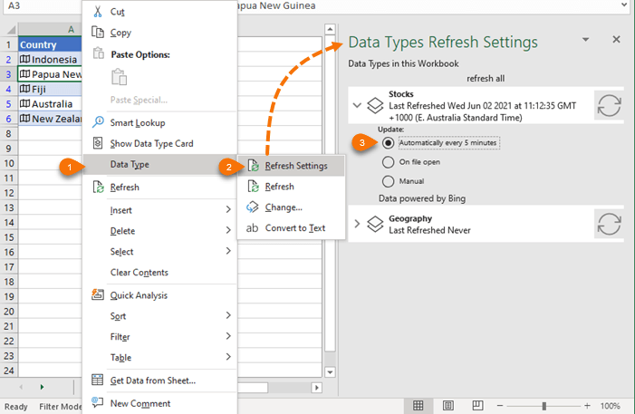
Refresh Settings — New June 2021
Via the right-click menu you can set the data types to automatically refresh every 5 minutes, on file open, or manually:
Data Type #FIELD! Error
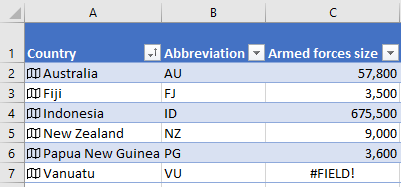
If the data doesn’t exist for a card Excel will return the #FIELD! error, as you can see below for Vanuatu’s armed forces size:
Convert to Text
Copying and pasting data type cells as values will retain the cards. To convert the data types to regular text, right-click > Data Type > Convert to Text:
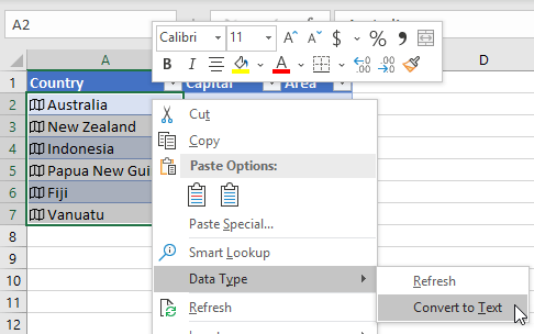
Tip: Notice you can also refresh the cards here.
Other Data Types
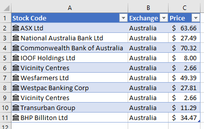
So far, we’ve looked at countries, but Excel also supports zip codes/postcodes, cities, stocks, index funds and other financial data. The example below are stocks on the Australian Stock Exchange:
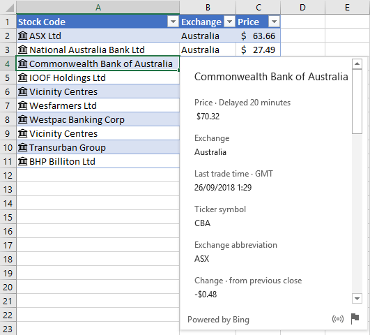
Opening the card gives you a list of the data you can retrieve and how long ago it was updated:
More to Come
The Excel team have big plans for Data Types with more coming, including the ability to create your own data types unique to your organisation. Imagine data types for Employees, Products, Stores, Regions… the list is endless.
Please Share
If you liked this please click the buttons below to share.


Simon Hurst explores the benefits of using Excel Data Types for easy-to-create management accounts.
The potential of Data Types and where to find them in Excel
When I first read about the ability to create Excel Data Types using Power Query, I probably over-estimated its potential. Having thought about it a bit more and experimented with creating Data Types, I have downgraded my initial assessment from earth-shattering to quite interesting. However, it’s certainly still worth investigating. Note that this feature is currently available to Office Insiders as a Preview so, depending on the upgrade channel you have chosen, it might not yet be available in your version of Excel.
For those who have not yet come across Data Types in Excel, these are a relatively recent addition to the Data Ribbon tab. The new Data Type group includes two built-in Data Types: Stocks and Geography. The basic idea is that you can designate the contents of a cell, or perhaps more usefully an entire Excel Table column, as being one of the available Data Types. Then, for the built-in Data Types, Excel will check the cell entry or entries and, if it can identify them as being a valid item within that Data Type, will allow for further values or columns of values to be filled in by looking the values up online:
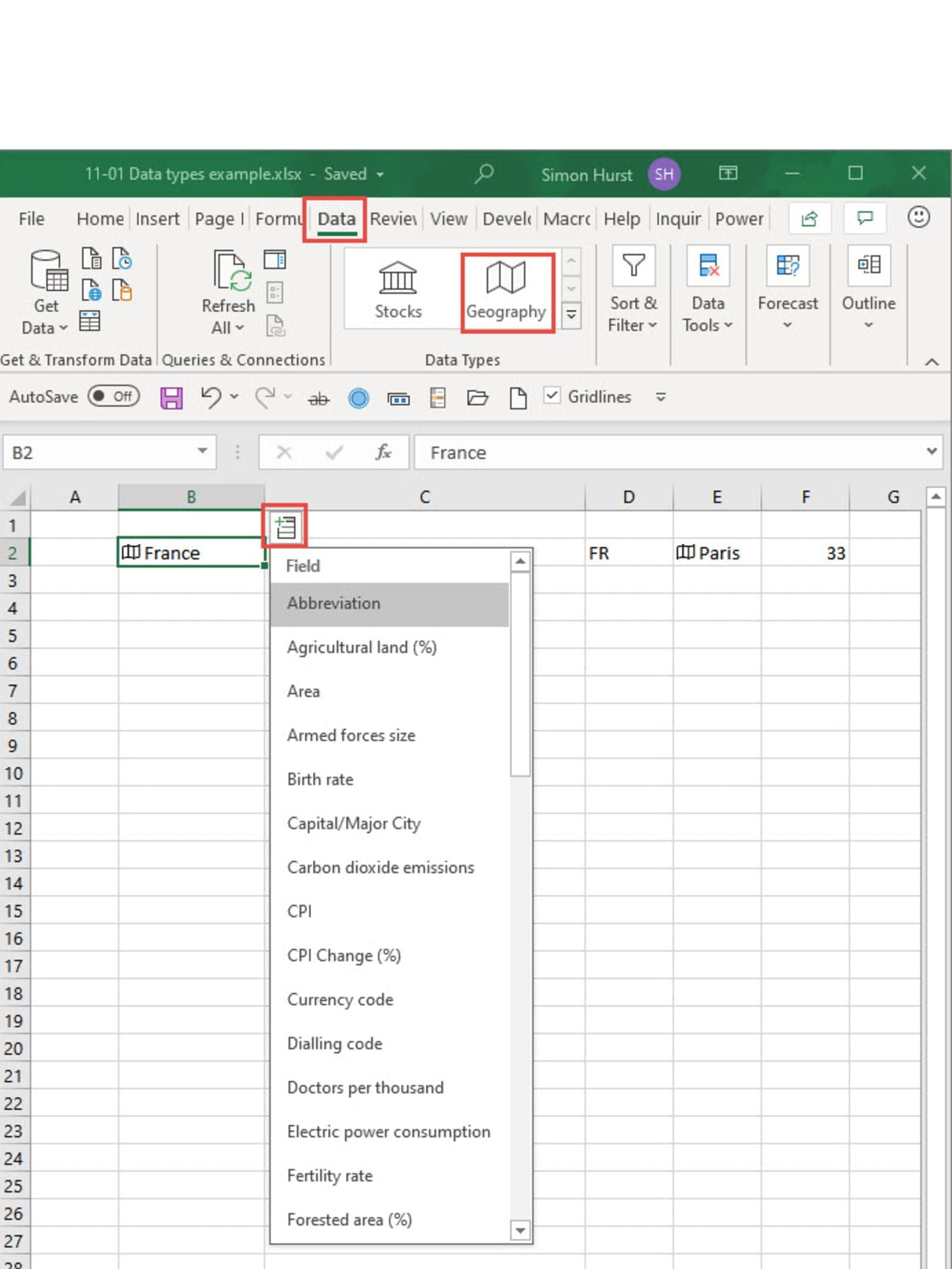
Several Excel Community Archive articles cover Data Types in more detail but, at the time of writing, it is not possible to search for any of them.
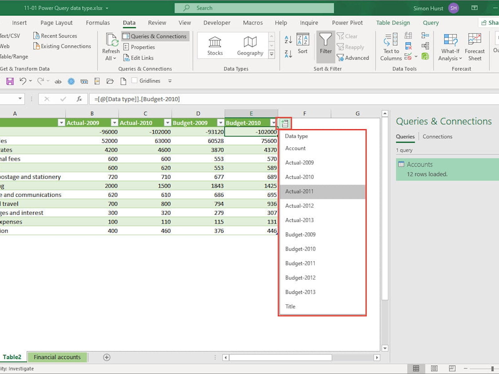
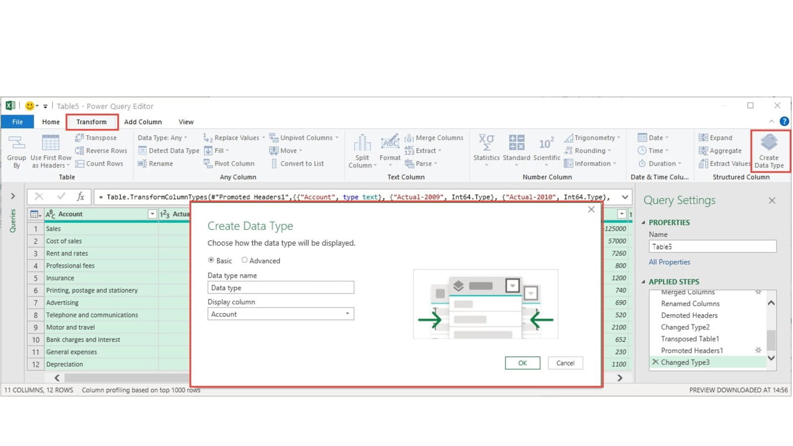
The new Data Type preview feature allows a Power Query query to be used as the source of Data Type values. The creation of such a Data Type is straightforward. Within the Power Query editor, you select multiple columns and use the Transform Ribbon tab, Structured Column group, Create Data Type option. This collapses the selected columns into a single column. Once the query with the collapsed column is loaded to a worksheet table, the column behaves in a similar way to one of the built-in Data Types allowing the user to choose which of the collapsed columns to display:
The above example is based on extracting columns from an Excel worksheet and then reorganising them so that they can be used as part of the Data Type. Here is the original worksheet:
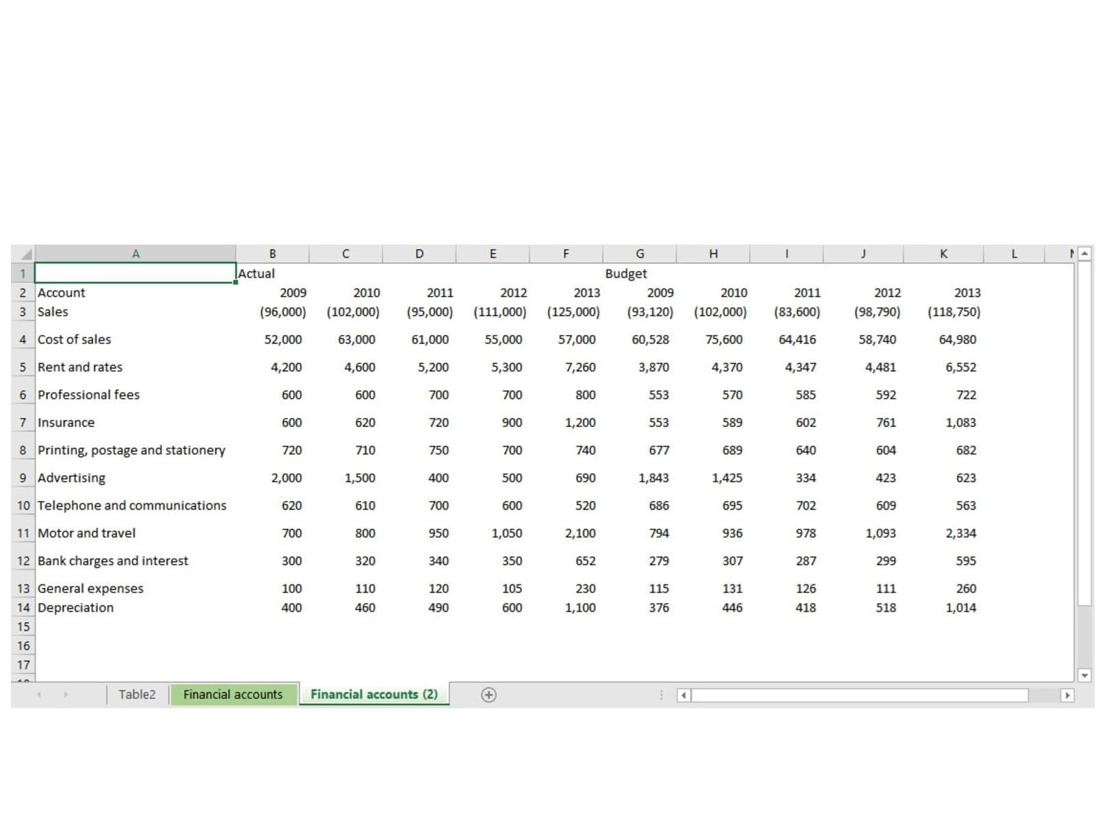
Given that the process of creating our Data Type is so straightforward, we’ll also cover a couple of other useful Power Query techniques. First of all, we need to click on any cell in our data and choose the Data Ribbon tab, Get & Transform Data group, From Table/Range option. This will convert our data into an Excel Table and ask whether our Table has headers. We will leave this option set to no.
Here is our data in the query editor. Our first task is to sort out the headers which are not currently in an ideal format. We want to do this in a way that makes the process as automatic as possible, rather than just treating the first row as a header row and changing the column names manually. Accordingly, we will use the Transform Ribbon tab, Table group, Transpose option:
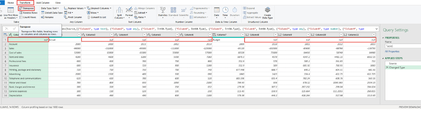
This is our query with the rows and columns transposed:
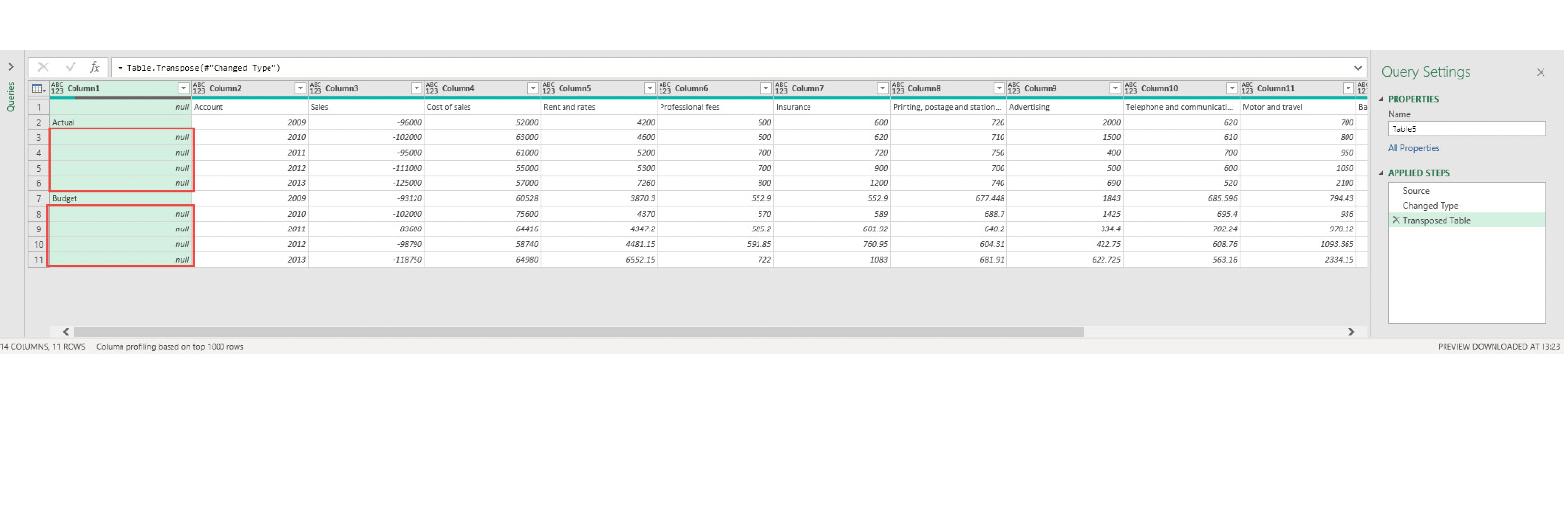
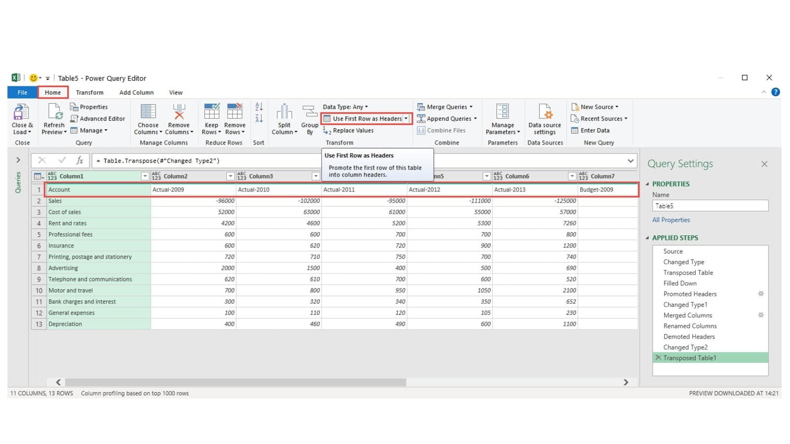
With our query transposed, we can right-click in our first column heading and use Fill, Down to copy the Actual and Budget headings to the rows beneath them that contain null. We can then use the Home Ribbon tab, Transform group, Use First Row as Headers option to promote our first row to become the table headers:
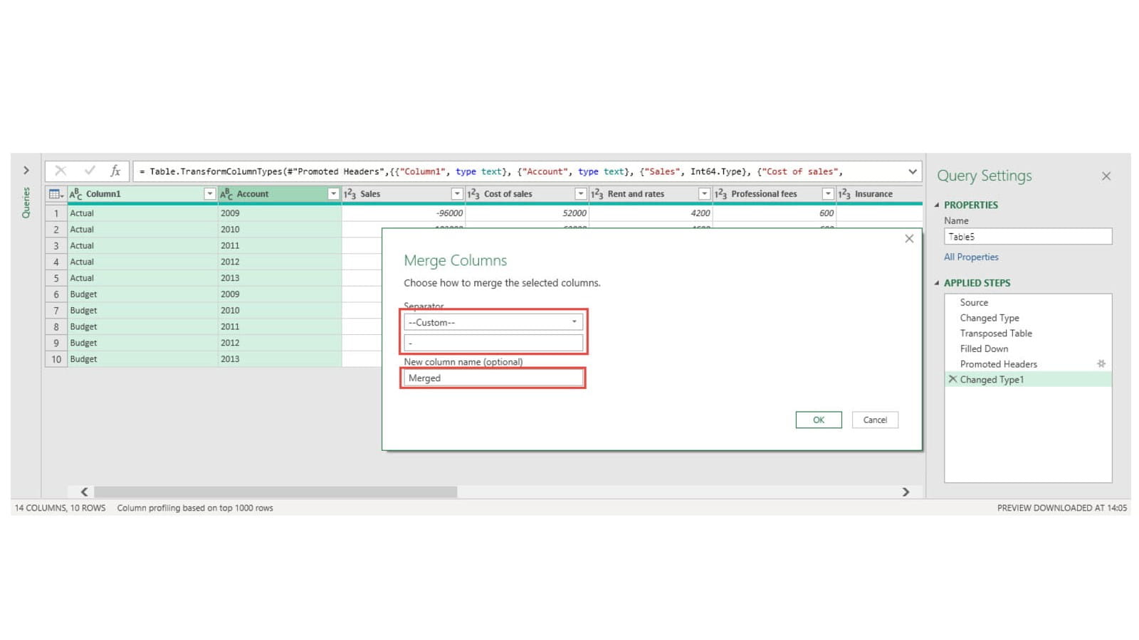
We want to combine Column1 and Account to form the column headings for our Excel Data Type so we select the two columns, right-click in either column header and choose Merge Columns. We have set the Separator to Custom and entered the dash as our custom separator. We leave the name of the new column at the default of Merged, because one of our columns is already called Account. We can then rename our Merged column heading to Account after the Merge step is complete:
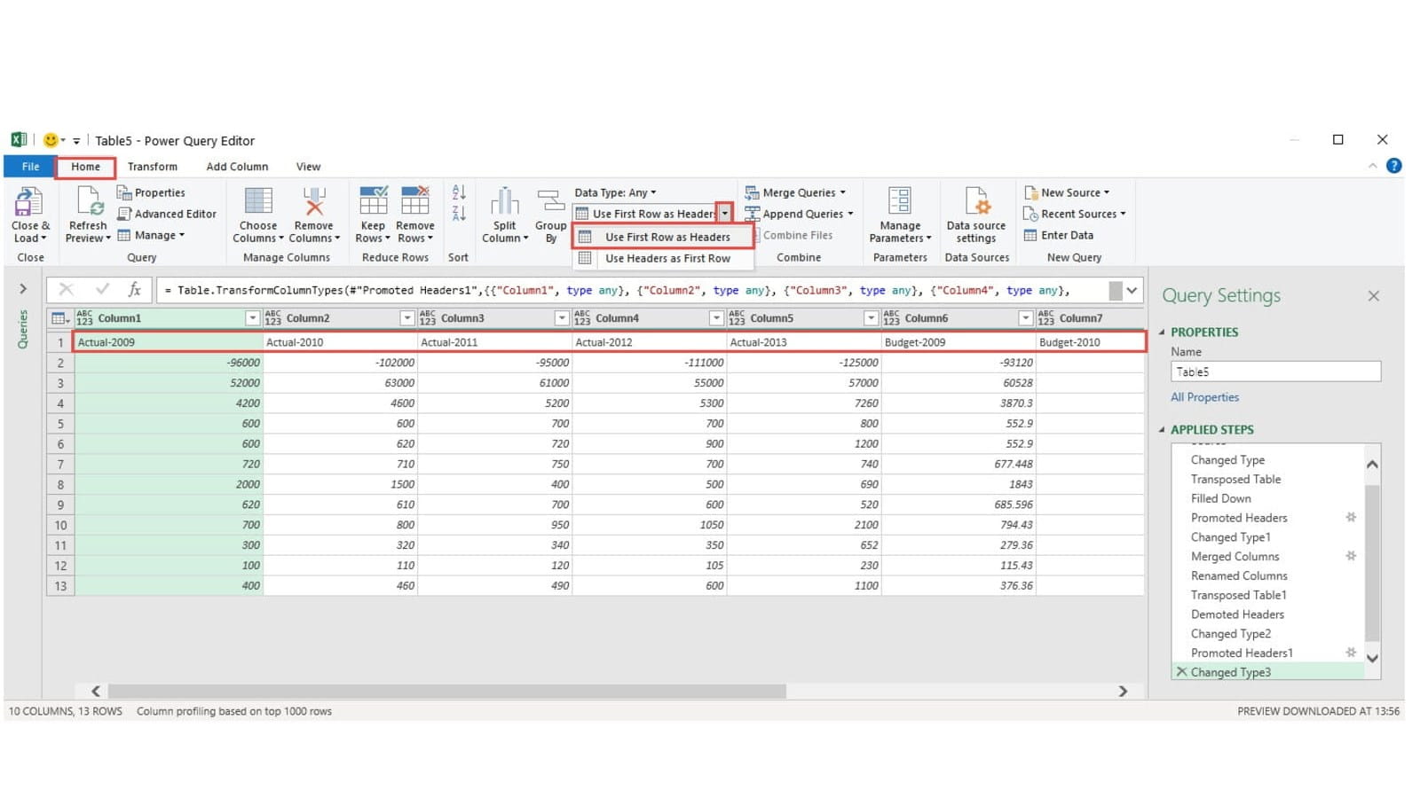
In order to allow our Excel Data Type to access our budget and actual columns, we will use the dropdown of the Use First Row as Headers option to select the antithetical Use Headers as First Row. We can then use Transpose, before resetting our headers using Use First Row as Headers:
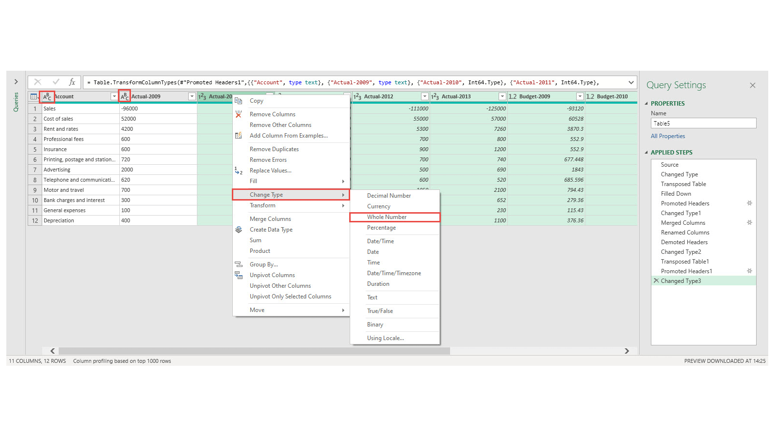
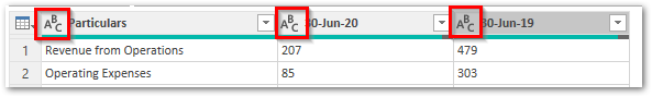
Next, we can change our column data types to Text for our first two columns and Whole Number for all the others. We can change individual column data types by clicking on the data type icon at the left-hand side of the column header. To change the data types of multiple columns, select all the columns required using Control+Click or Shift+Click, then right-click in any of the selected column headings and choose Change Type:
Lastly, we select all of our columns and use the Transform Ribbon tab, Structured Column group, Create Data Type command to collapse all of our value columns into a single Account column:
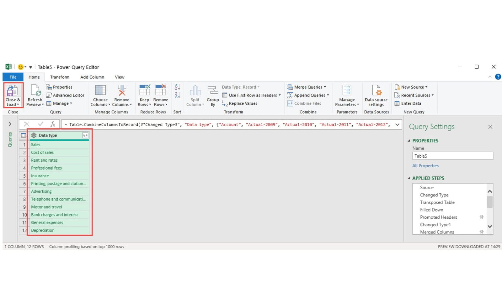
This collapses our individual columns into a single, structured, Data Type column and we can then use Close & Load to load this single-column Table into an Excel worksheet:
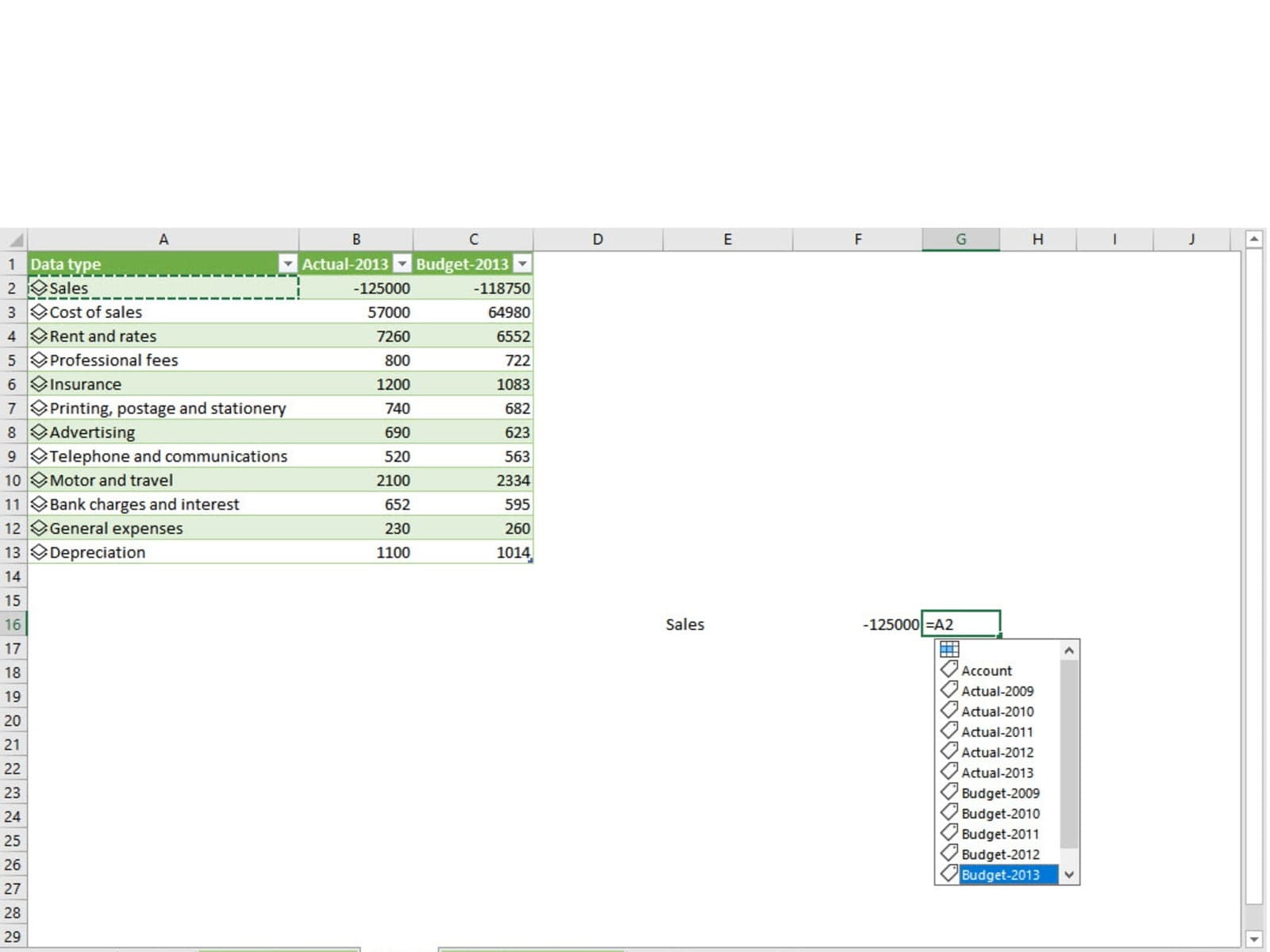
When we load a query with a Data Type column to our worksheet, Excel recognises the data column and displays the Data Type symbol. We can then click in the column to display the list of available items and we just have to choose whichever of our actual or budget columns we want to display to add it to our Table:

In addition, we can refer to our Data Type column items from a cell outside our Table, and choose which of the available Data Types to use:
Excel Power Query is a powerful inbuilt tool provided by Microsoft in Excel versions 2016 and higher. The power query feature allows you to get and extract data from multiple internal and external sources to Excel. This feature imports the data from the source to excel and displays it in an excel table format. As it creates an excel table, the column header data types play a very important role in Excel Power Query.
In this tutorial, we would learn everything about the data type, its importance, and what happens if you do not give ignore the power query header data type. We would also unlock multiple ways to change the data type of table headers in power query.
Table of Contents
- Power Query Data Types – Meaning and Types
- Background – Power Query Data Types
- Where Can I Check Table Data Types?
- How To Change Data Types in Power Query?
- Enable or Disable – Automatically Detect Data Types
Power Query Data Types – Meaning and Types
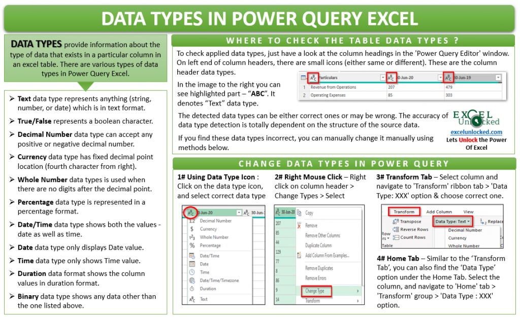
The term Data Types is quite a self-explanatory word. Data Types provide information about the type of data that exists in a particular column in an excel table. There are various data types available in the power query, listed below
- Text – The text data type represents anything (string, number, or date) which is in a text format.
- True/False – This represents a boolean character (value is either True or False).
- Decimal Number – This data type can handle any decimal number (negative or positive) with any number of digits after the decimal point. It also accepts a whole number (without decimal digits).
- Currency – Unlike the Decimal Number, the Currency data type has a fixed decimal point location which is at the fourth character from the right. Another name of this data type is Fixed Decimal Number.
- Whole Number – This numeric data type is generally used when you are not sure about the number of digits. It can accept positive or negative integer number with 19 digits. In the case of whole numbers, there are no digits after the decimal point.
- Percentage – Percentage is similar to the Decimal Number data type. However, it represented in a percentage format.
- Date/Time – The column formatted as Date/Time shows both the values – date as well as time.
- Date – This data type only displays the Date value.
- Time – This data type only shows the Time value
- Date/Time/TimeZone – When you apply this data type to a column, you would see the data having all – date, time as well as the time zone.
- Duration – This data format shows the column values in duration format.
- Binary – This shows any data other than listed above.
Background – Power Query Data Types
When you import any table data into a power query, you would notice that the power query automatically performs some pre-defined steps on the imported data. One of these default steps is the ‘Changed Type‘ step.
In this step, the power query intelligently understands the content of the imported data and detects/applies the data type to the column based on the first 200 values in each of the columns.
For example – Let’s say, if a particular column in the imported data contains date values, then the power query would detect this data and change the data type of the column to ‘Dates’. Likewise, if a column contains only string characters, then it would smartly convert the data type to ‘Text’.
Where Can I Check Table Data Types?
To check the applied data types, just have a look at the column headings in the ‘Power Query Editor’ window. On the left end of the column headers, you would notice small icons (which may be either the same or different in each of the columns). These are nothing but the intelligently detected table column data types.
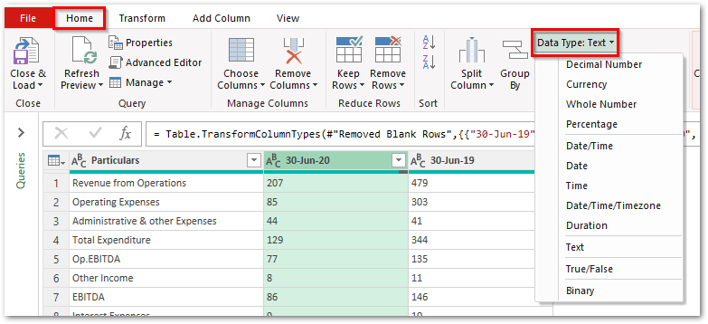
In the below image you can see the icon as ‘ABC’. This denotes the ‘Text’ data type for the three columns.
You can use the ‘Detect Data Type’ option on the ‘Transform’ tab (in Power Query Editor window) to help excel automatically detect the data types for your table headers, as shown below:
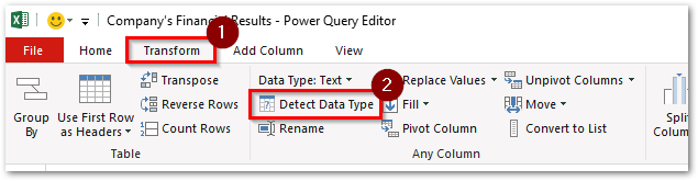
The detected data types may be the correct one or maybe wrong. The accuracy of data type detection is totally dependent on the structure of the source data. As in the above image, you can see that the table values for column B and C is numeric, however, the detected data type is ‘Text’.
If you find these data types incorrect, you can manually change it by following any of the below methods.
How To Change Data Types in Power Query?
There are multiple ways to change or manually update the power query data types.
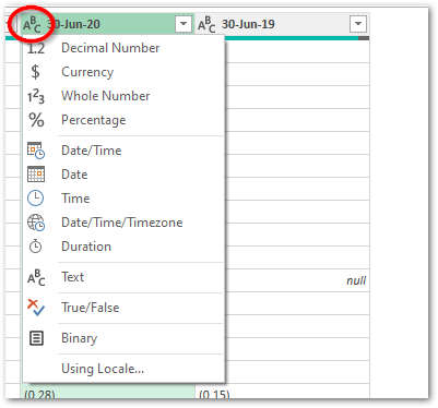
- Using Data Type Icon – Click on the data type icon, and select the correct one, as shown below:
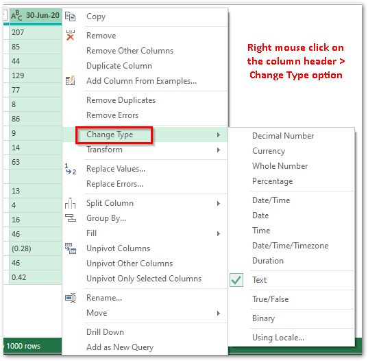
- Column Header Right Mouse Click – Simply select right-click on the column header. From the list of options, go to the ‘Change Type’ and select the appropriate data type, as shown below:
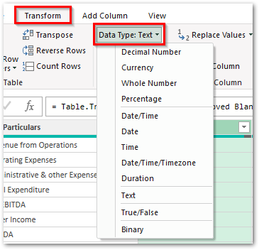
- Transform Tab – Select the column, and navigate to the ‘Transform’ ribbon tab > ‘Any Column’ group > ‘Data Type: XXX’ option and choose the appropriate type from the list.
- Home Tab – Select the column, and navigate to the ‘Home’ tab > ‘Transform’ group > ‘Data Type : XXX’ option and choose the appropriate type from the list.
Enable or Disable – Automatically Detect Data Types
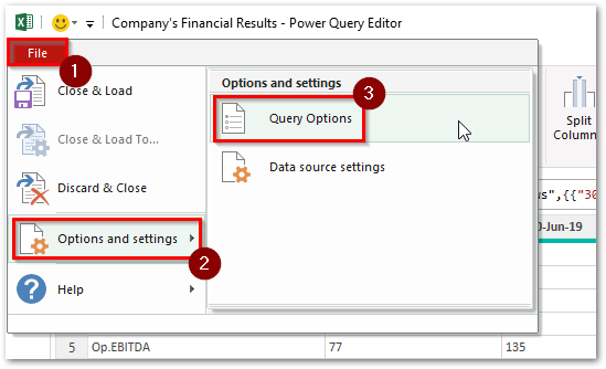
The automatic detection of data types in power query is by default enabled. To switch or turn on automatic detection of power query data types, simply follow this path – Go to the ‘Power Query Editor’ window and then navigate to File > Options and Settings > Power Query Options as shown below:
In the ‘Query Options’ dialog box that appears, choose the second radio button (under ‘Type Detection’ section).
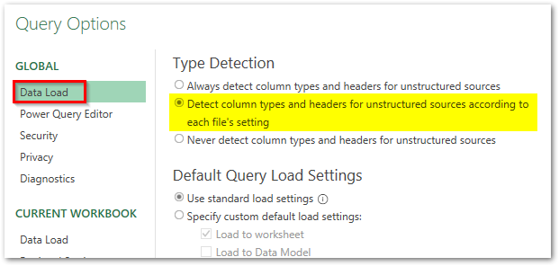
On enabling it, power query would do two steps by default.
- Firstly, it would promote the first row of the data as column headers.
- Secondly, it would detect and change the data types for the column header. The detection of correct data types is totally based on how the first 200 rows of the data are structured.
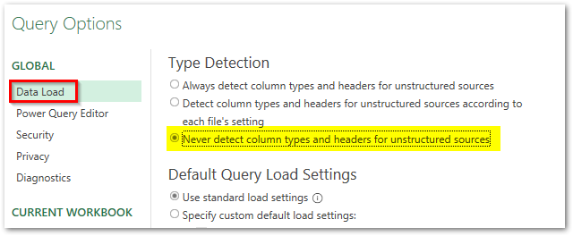
To disable or turn off automatic data type detection, select the third radio button – ‘Never detect column types and headers for unstructured sources‘ as highlighted below.
With this, we have reached the end of this tutorial. Write your feedback on this page in the comment box below.
RELATED POSTS
-
How to Filter and Sort Data in Excel Power Query
-
Install Power Query in Excel 2010 [Step by Step Guide]
-
Overview of Power Query in Excel
-
How to Import Data from Text File or Notepad to Excel
-
How to Unpivot Data in Excel Using Power Query
-
Group and Summarize Data in Excel Power Query
Change data types in Datasheet view Access opens the table in Datasheet view. Select the field (the column) that you want to change. On the Fields tab, in the Properties group, click the arrow in the drop-down list next to Data Type, and then select a data type. Save your changes.
Contents
- 1 How do you change the datatype in Excel?
- 2 How do you find the data type in Excel?
- 3 How do you change the cell type?
- 4 How do I change data values in Excel?
- 5 How do I remove data type in Excel?
- 6 Which of these is not the data type in Excel?
- 7 What is the default data type in Excel?
- 8 How do you change the cell type in excel in Java?
- 9 How do I get data from sheet 1 to sheet 2?
- 10 How do I change text to #value in Excel?
- 11 What is an Xlookup in Excel?
- 12 How do I convert data to text in Excel?
- 13 How do I delete just the text in Excel?
- 14 How do I remove text from columns in Excel?
- 15 Which of the following is mutable data type?
- 16 Which of the following is valid data type in Excel?
- 17 What is Pivot in Excel?
- 18 How do I enable linked data in Excel?
- 19 What is string Data Type in Excel?
- 20 How do I get to preferences in Excel?
How do you change the datatype in Excel?
To avoid this from happening, change the cell type to Text:
- Open the Excel workbook.
- Click on the column heading to select entire column.
- Click Format > Cells.
- Click the Number tab.
- Select “Text” from the Category list.
- Click OK.
How do you find the data type in Excel?
Go to the Formulas tab and select More Functions > Information > TYPE.
How do you change the cell type?
Setting Cell Type in Excel 2010
- Right Click on the cell » Format cells » Number.
- Click on the Ribbon from the ribbon.
How do I change data values in Excel?
Converting formulas to values using Excel shortcuts
Just follow the simple steps below: Select all the cells with formulas that you want to convert. Press Ctrl + C or Ctrl + Ins to copy formulas and their results to clipboard. Press Shift + F10 and then V to paste only values back to Excel cells.
How do I remove data type in Excel?
Select the cells, rows, or columns that you want to clear. Tip: To cancel a selection of cells, click any cell on the worksheet. , and then do one of the following: To clear all contents, formats, and comments that are contained in the selected cells, click Clear All.
Which of these is not the data type in Excel?
Explanation: Excel has three types of data types : values, labels and formulas but does not have any data type named as character.
What is the default data type in Excel?
Whole value: If the data is a whole value, such as 34 or 5763, Excel aligns the data to the right side of the cell. Value with a decimal: If the data is a decimal value, Excel aligns the data to the right side of the cell, including the decimal point, with the exception of a trailing 0.
How do you change the cell type in excel in Java?
Apache POI Excel Cell Type Example
- package poiexample;
- import java.io.FileOutputStream;
- import java.io.OutputStream;
- import java.util.Calendar;
- import java.util.Date;
- import org.apache.poi.hssf.usermodel.HSSFWorkbook;
- import org.apache.poi.ss.usermodel.CellType;
- import org.apache.poi.ss.usermodel.Row;
How do I get data from sheet 1 to sheet 2?
Here’s how:
- Select all the data in the worksheet. Keyboard shortcut: Press CTRL+Spacebar, on the keyboard, and then press Shift+Spacebar.
- Copy all the data on the sheet by pressing CTRL+C.
- Click the plus sign to add a new blank worksheet.
- Click the first cell in the new sheet and press CTRL+V to paste the data.
How do I change text to #value in Excel?
To replace text or numbers, press Ctrl+H, or go to Home > Find & Select > Replace.
- In the Find what box, type the text or numbers you want to find.
- In the Replace with box, enter the text or numbers you want to use to replace the search text.
- Click Replace or Replace All.
- You can further define your search if needed:
What is an Xlookup in Excel?
Use the XLOOKUP function to find things in a table or range by row.With XLOOKUP, you can look in one column for a search term, and return a result from the same row in another column, regardless of which side the return column is on.
How do I convert data to text in Excel?
Use the Format Cells option to convert number to text in Excel
- Select the range with the numeric values you want to format as text.
- Right click on them and pick the Format Cells… option from the menu list. Tip. You can display the Format Cells…
- On the Format Cells window select Text under the Number tab and click OK.
How do I delete just the text in Excel?
1. Select the cells you need to remove texts and keep numbers only, then click Kutools > Text > Remove Characters. 2. In the Remove Characters dialog box, only check the Non-numeric box, and then click the OK button.
How do I remove text from columns in Excel?
1 Answer. Select any cell with a value and run Data ► Text-to-Columns, Delimited. Turn off all delimiters and click Finish.
Which of the following is mutable data type?
9. Which one of the following is mutable data type? Explanation: set is one of the following is mutable data type.
Which of the following is valid data type in Excel?
Following are the valid data types in excel: 1)Labels:- Labels (text) are descriptive pieces of information, such as names, months, or other identifying statistics, and they usually include alphabetic characters. 2)Values:- Values (numbers) are generally raw numbers or dates.
What is Pivot in Excel?
A pivot table in Excel is an extraction or resumé of your original table with source data. A pivot table can provide quick answers to questions about your table that can otherwise only be answered by complicated formulas.
How do I enable linked data in Excel?
In Excel, click the File tab.
Change settings for Linked Data Types
- Enable all Linked Data Types (not recommended) Click this option if you want to create linked data types without receiving a security warning.
- Prompt user about Linked Data Types This is the default option.
What is string Data Type in Excel?
A text string, also known as a string or simply as text, is a group of characters that are used as data in a spreadsheet program.By default, text strings are left-aligned in a cell while number data is aligned to the right.
How do I get to preferences in Excel?
Click the Excel menu. Select Preferences. Select General.
Having represented this site as a technology blog with a focus on programming and software development, I find myself starting off with a tutorial on Excel basics instead. Somehow, I thought it was going to be more glamorous than this . . . This is driven by my need to prepare a training for my staff at work, and in keeping with the DRY principle (Don’t Repeat Yourself) I am killing two birds with one stone. Anyone hoping to read programming stuff is just going to have to wait . . .
This is part two of a multi-part series targeting entry-level users of Microsoft Excel. In the previous post, we discussed the basic structure of a spreadsheet, and covered the vary basics of using expressions (or formulas). There is a LOT more to that, but before we go any further, it is important to understand how Excel understands data.
I am about to be a little long-winded. Hopefully you will slog through anyway, unless you already have a solid grasp on this stuff. Let’s take a (really) broad look at some data basics, before we explore the data type definitions specific to Excel. Because this is a long post, here are some navigation aids:
The Broad View – Information Basics
- What’s in a number? (numeric information)
- Truth Be Told (logical information)
- String Theory (Text information)
Details of Excel Data Types
- The Logical Data Type
- The Number Data Type
- The Text Data Type
- The Error Data Type
What’s in a number?
We humans don’t tend to think too hard about the type of data we are working with. We have evolved to be context-aware, and as we learn, we understand how to use MOST information within a particular context. For example, when we talk about our Social Security number, or our credit card number, we generally recognize either of those things as an identifier composed of numerical characters. We do not expect to be performing addition, multiplication, or other mathematical operations on these, even though semantically we still call them “numbers.” Further, both SSN’s and Credit Card account numbers might contain one or more leading zeros, or zeros at the rightmost end of the numerical sequence:
Example SSN: 001-11-1111
Never mind the dashes which make this SSN format behave emphatically NOT like a true number.
While most credit card companies assign a string of numerals as an account identifier (account number), other business entities might use a mixture of numerals and alphabetical characters to create account identifiers, which we still tend to refer to as “account numbers.” Again, while we think of the various account identifiers which (for some) rule our lives as “numbers”, we also tend to utilize them in a context more like a string of characters.
Contrast this with Social Security payments and/or credit card charges. These numbers represent numerical values which we contextually understand will be added to or subtracted from the current balance of our account. In a similar manner, the credit company will most likely perform a calculation (which, apropos of nothing whatsoever, would be represented by a formula) to determine how much interest to charge to our account. This amount would be calculated based upon our current balance (and a number of other factors), and then added to that balance for the current billing period. We intrinsically understand this, even though the actual math part may not be a part of our conscious thought stream.
In these cases, our human contextual ability allows us to (most of the time) use the right “numbers” in the correct and meaningful manner. Mentally, we all might play a quick mental arithmetic on our credit card account balance, subtracting the approximate amounts of our recent charges, before we decide to purchase that new 52″ HD television. When we whip out the plastic to punch the card number into the space on the Amazon website, we type in the set of numbers, recognizing that there is no numerical operation to be performed, other than making sure we type correctly.
[Back to Top]
Truth be Told . . .
On the other hand, we humans are nowhere near as good at evaluating a set of conditions and arriving at a concise logical value. We have to practice at this, and even then, our ability to inject that very same context can create flaws in our evaluation. We confuse our singular perceptions with absolutes. True logic is not relative. For example, on a very cold day here in Portland (say, 37 degrees F – yes, that would be “cold” here in the Pacific Northwest) one man might observe to another that it is “freezing out here” when in fact the temperature is well above the point at which liquid water changes state into its solid form. However, his companion is very likely to agree with him, or failing that, state that “yup, it’s cold out.”
Neither of these statements can be evaluated from a logical standpoint outside that of the observer, because they are relative statements. If an Inuit fresh from the North Slope of Alaska were to join the group, he would likely find the observations of the other two men absurd. To the Inuit, the actual outdoor temperature of, say, 37 degrees might feel nearly tropical. In fact, since “freezing” is technically defined as the point at which water turns to ice (32 degrees Fahrenheit, or 0 degrees Celsius), the only valid logical statement which could be made in this situation is that it is NOT, in fact, freezing outside.
As humans, we are accustomed to applying our personal, regional, and societal metrics in evaluating information. Our computers, however, and by extension the software which runs on them, are machines which deal in absolutes. To the machine, a statement which is not 100% true is FALSE. Numbers may be manipulated in meaningful mathematical ways, while arrangements of text cannot (or at least, not in the same manner as true numbers).
Despite some illusions built into our modern software (including Microsoft Excel) to the contrary, the computer does not understand context. The computer is very, very literal and will perform whatever action or calculation you request of it (unless, of course, the programmer built in a mechanism to prevent the operation from being carried out if certain conditions aren’t met) with no comprehension of the sensibility of the result.
At the very, very most basic level, TRUE and FALSE (in a technical sense, ON and OFF) are the only two things the computer hardware understands. After one delves down through several layers of software abstraction, one eventually runs into hardware which is binary in nature. Binary code is composed of ones and zeros, representing ON (one) and OFF (zero). We are not going to go into how all THAT works here. But its important to understand the literal nature of the machine, that the machine lacks ANY “context” beyond that supplied by the programmer, and that all of the information we work with in our user-friendly, usability-tested software interface has been heavily abstracted for our benefit.
There is an entire branch of mathematics devoted to logical analysis called Boolean Algebra. While we won’t be going into that in this article, an understanding of basic logical operations can lend itself well to some advanced spreadsheet features that will make you the envy of your friends, and the champion around the office. More in a bit.
[Back to Top]
String Theory
I am NOT about to embark on a discussion of theoretical physics.
I am going to talk about text. Like, words. This overly long post is constructed of words, in the English language, which I have typed in to the computer using my keyboard. I am currently creating this post using Windows Live Writer, a nifty blogging program which has abstracted away the need for me to understand all that goes into marking up my blog post with suitable HTML, creating an ftp connection, and uploading the content into the proper directories on the server so that it displays properly for you, the reader. I just type, and when I am done, I use mu mouse cursor to push an on-screen representation of a “button” that says “publish”. In the same manner, our software tends to abstract from us the need to understand what is really going un “under the hood” when we ask our machines to work with text. It appears to us, as end users, that the machine recognizes the strings of characters we type and manipulate, and works with text just as easily as it works with numbers.
Which is emphatically not true.
We’re not going to go into the how and why of it right now, but let’s just say that creating effective ways for our machines to handle input, display, formatting, and printing of text (not to mention standardization across platforms!) has been one of the major challenges of the PC era. Just to give you an idea, here are a couple of entertaining and informative articles by Joel Spolsky on the topic of character strings. It is not required reading for our purposes here, but you may find it informative:
- Back to Basics (aka The Schlemiel the Painter Article)
- The Absolute Minimum Every Software Developer Absolutely, Positively Must Know About Unicode and Character Sets (No Excuses!)
Suffice it to say, it is important to be aware that text information lives in its own realm, even within the confines of our simple spreadsheet. Even more important, it is REALLY important for you, the reader, to be able to properly distinguish whether your spreadsheet should be treating the information in a cell as text, or something else. We’ll see why in the next post.
A final comment before we get into the nitty gritty. At a basic level, the text we take for granted on screen is regarded by our machine as a string of characters. These characters are actually ASCII or Unicode representations of what we actually see displayed. Because our words, sentences, and paragraphs (including whitespace and non-printing items such as carriage returns, tabs and other markup) are all composed of such character strings, we will often refer to text data as strings. In other words, in your travels, whether in Excel or some other application, mention is made of “String Parameter”, “String Data Type”, etc. you can generally substitute “text” for “string” and be just fine.
Ok. Now that we have the preliminaries out of the way, let’s look at how Microsoft Excel regards our data.
[Back to Top]
Data Types
Microsoft Excel recognizes four kinds of information: Logical values (TRUE or FALSE, also called Boolean values), Numerical values, Text values, and Error types. The four kinds of information are known, in technical parlance, as Data Types. What is important for you, the user, is to begin to think of your own information in this manner, and consider how the machine is going to use it.
Note that Excel will do the very best it can to figure out which of these types it THINKS you intend, once you complete typing into a cell and hit the enter key. For example, if you type a series of numerals, it assumes you intend a number type. If that series of numerals happens to begin with one or more zeros, Excel STILL thinks you intend to type a number, and eliminates those leading zeros. Likewise, if you type something the looks like a date, and contains valid numbers which can represent a valid date, Excel assumes you mean a number type again, formatted as a date.
You will learn more about this date stuff later in the post. However, be aware that Excel tries to help you in this manner. Most of the time, it works out. Sometimes, it doesn’t, and then you have to help Excel by telling it what you REALLY mean, explicitly.
The Logical Data Type
Logical values are either TRUE or FALSE.
In most cases, logical values will be present as the result of the evaluation of an expression or function. Essentially, a logical value represents the resolution of an expression indicating whether certain conditions have been met. For example:
The statement “1 is less than 2” is recognizable as a true statement. Another way to put that is:
1 < 2 = TRUE
When evaluating logical expressions, Excel recognizes the text TRUE as a logical (or boolean) value. Excel also treats the value 0 as false, and any other numerical value as true. For example, we can make a logical comparison about the values in two different cells by typing an expression:
If we add change one of the values, the expression will no longer return true:
Logical expressions are one of the more powerful tools Excel has to offer, and yet they are also some of the least utilized. We will devote an entire post to examining logical expressions in the near future.
[Back to Top]
The Number Data Type
Numerical values are, of course, numbers. This is more complex than it first appears, however. First of all, Excel stores all numbers as Double-Precision Floating Point values. I know. It’s a mouthful. For our purposes here, you can think of that as a decimal number, with room for a lot of decimal places if needed. Excel can store numbers as large as 1.79768 X 10308 and as small as 2.2250 X 10-308. These represent extremely large, and extremely small numbers, respectively.
The thing to remember here is that to Excel, all of the following are numbers: 15,000; 100; $50; $50.00; 75%; 0.5; 5.35E+04; and 12/25/2012.
What, you say? What was that last? Yes. To Excel, dates are also stored as plain old numbers. We’ll discuss THAT in a minute. For the moment, take a look at what you might type in or see displayed in a cell, vs. what excel is actually storing:
| Visible in Cell | 15,000 | 100 | $50,000 | $50.00 | 75% | .5 | 5.35E+04 | 12/25/2012 |
| Number Stored | 15000 | 100 | 50000 | 50 | 0.75 | 0.5 | 53500 | 41268 |
While you are likely familiar with most of the numbers you see in the table above, some of you may not be familiar with the second from the right, known as Scientific E notation. Don’t worry about that right now. Scientific E notation is a a sort of shorthand for expressing very large (or very small) numbers The example above is trivial for the purpose of illustration. Trust me that the expression in the top cell is numerically equivalent to the number displayed in the cell below.
The important thing to remember is that numbers in Excel can be no more than 15 significant digits in length. This excludes zeros on either side of the number:
99999999999999900000 is 20 numerals, but only contains 15 significant digits; the fifteen “9’s” to the left of the five zeros. Likewise, .00000999999999999999 is also twenty decimal places, but contains only fifteen significant digits).
Numbers which are entered that contain more than 15 significant digits will be truncated. That is, significant digits will be lopped off the right-hand side and replaced with zeros. Note in the examples below, we can type in 19 significant digits (fourteen 9’s followed by 87654). Once we hit “Enter”, the significant digits in excess of 15 are truncated, leaving 0’s):
Dates and Times
Ok. Now on to that date thing. Dates and times are also stored as number types by Excel. Dates are stored as the number of days since the date 1/1/1900. In other words, January 1, 1900 is considered by Excel to be 1. Therefore, 1/2/1900 would be stored as 2, 1/3/1900 as 3, and so on. Note that Excel does not recognize dates BEFORE 1/1/1900. We’ll see why this matters in the next post about functions and expressions.
Excel treats Times as fractions of days. Since a day is 24 hours in length, then 1/4th of a day (0.25) would be 6 hours. Since each day begins at 0 hours and 24 hours later, Excel would store the date and time for 6:00 AM on 1/1/1900 as 1.25. As I type this sentence, it is 10:39 PM on August 9th, 2011. Therefore, Excel would store the current date and time as 40764.94384. That is, forty thousand three-hundred eighty-four and (roughly) 94/100ths days since 1/1/1900.
Values vs. Formats
The key thing about numbers in Excel is that you need to separate in your mind the number VALUE from the way it is DISPLAYED. The manner in which Excel displays a given numerical value within a cell is known as formatting. We will discuss different aspects of number formatting later, but for the moment, keep in mind that underneath whatever window dressing Excel provides in terms of formatting, the following are all representations of the same value (1.05):
1.05 = 1.050000 = $1.05 = 105% = 1/1/1900
| Value in Cell | Format | Displayed in Cell |
| 1.05 | General | 1.05 |
| 1.05 | Number (6 digit decimal precision) | 1.050000 |
| 1.05 | Currency | $1.05 |
| 1.05 | Percent | 105% |
| 1.05 | Date | 1/1/1900 |
Likewise, these ALSO represent the same numerical value (.75):
.75 = $0.75 = 75% = 3/4 = 6:00:00 PM
| Value in Cell | Format | Displayed in Cell |
| 0.75 | General | 1.05 |
| 0.75 | Currency (2 digit decimal precision) | $0.75 |
| 0.75 | Percent (1 digit decimal precision) | 75.0% |
| 0.75 | Fraction | 3/4 |
| 0.75 | Time (hh:mm PM) | 6:00:00 PM |
We’ll cover the ins and outs of the various formatting choices in the next post. But be aware, that formatting can be tricky. Notice how, in the first example above, if we choose to format the value 1.05 as a Date, we get the displayed value of 1/1/1900. In a way, this is to be expected, since we learned that in Excel, the number 1 can be considered to represent 1/1/1900. But what about that .05 (five one-hundredths)? Well, this would actually represent 1/20th of 1 day (5/100ths reduces to 1/20th). But since we specified a date format which did not include the time as part of the format to display, we get only the date.
The value of a number is stored in the cell. Formatting determines how the number is displayed, and what level of precision is displayed. When using the value of the cell in calculations, the true value is used, not the displayed value!
We will see how this might matter in a later post. For now, we will move on the the Text data type.
[Back to Top]
The Text Data Type
As we discussed previously, Microsoft Excel regards test as strings of characters. The letters of the alphabet, numerical characters, symbols such as % and $, as well as spaces and tabs are all valid text. In cases where Excel cannot distinguish a value as either a number type, a logical type, or an error type, the value will be treated as text.
Excel will recognize a text string of up to 32,768 characters. However, only 1024 can be displayed in a cell.
Excel tries to be helpful, in that, as you enter information into a cell, the application attempts to determine what type of data you are entering and treat it accordingly. Most of the time this is fine, and helpful. However, sometimes it can trip us up. For example, we will return to the issue of leading zeros and account numbers. Lets say an account number begins with four zeros:00001234567891011. If we were to simply enter this string of numbers into a cell, excel will decide we are entering a number value, and will drop those leading zeros.
We can tell Excel to treat the data in a cell as text by pre-pending a single-quote character before the text we wish to enter, or by applying the text format to the cell through the cell formatting menu (which we will discuss in the next post).
Excel offers a host of text manipulation functions which we will examine in an upcoming post.
The Error Data Type
There are instances in which errors will occur when Excel evaluates the contents of a cell. For example, division by zero is mathematically undefined, and the machine cannot, by itself, resolve this error. It turns out the Excel has an Error type specifically for this instance, the #DIV/0! result.
The error type generally rears its ugly head due to problems with functions or formulas. The different error values Excel provides are listed in the following table, along with the meaning of the error:
| Error Value | Means | Common Causes |
| #DIV/0 | Division by zero | You attempted to divide by a value of zero. A blank cell is treated as zero in mathematical operations. |
| #N/A | No value Available | Manually entered (and sometimes when data is imported) to indicate information not available |
| #NAME? | Excel does not recognize the name of a list or range of cells | The #NAME? error will result if you neglect to enclose text in quotes within a formula, or if you refer incorrectly to the name (address) of a cell or range of cells. |
| #NULL! | Reference to a non-existent intersection between two cell ranges | If you neglect to separate to cell ranges with a comma in certain function arguments, the #NULL! Error will result. Also if you refer to an intersection between two cell ranges which do not intersect. |
| #NUM! | There is a problem with a number in a formula or result | Passing an invalid argument to a function or formula, or a formula returns a number which is too large or too small to be represented in the cell. |
| #REF! | Invalid Cell Reference | You have deleted or pasted over a cell or cells referred to in a formula. |
| #VALUE! | Invalid argument or operator in a function or formula | Usually results from performing a mathematical operation with cells that contain text. |
The short version of all this is that when you see that ugly hash symbol, you know you have a problem, usually in a formula. This reference will help you know where to begin looking for the problem.
OK. We’ve covered a lot of ground. In the next post we will take a closer look at formulas and some of the built-in functions Excel provides.
[Back to Top]
Summary
Understanding how Microsoft Excel interprets and handles different types of information is critical in constructing effective spreadsheets. Failure to properly anticipate how Excel will work with your data can potentially lead to calculation errors which are difficult to detect. In order to make the most effective use of expressions and formulas, and functions within Excel, an awareness of the various data types within the program will save time, frustration, and headaches.
- It is important to consider that the computer does not have a contextual understanding of our information, beyond what the programmers built in.
- Excel will attempt to determine the proper data type based on what you type into a cell. Sometimes you have to correct for this.
- Excel recognized four types of data;
- The Logical Type:
- Indicates a value of TRUE or FALSE
- A value of zero = FALSE; Any value other than zero = TRUE
- The Number Type
- All numbers are represented by a Double-Precision Floating Point value (big decimal numbers).
- Numbers may contain up to 15 significant digits (exclude zeros on either side of the number).
- Numbers may be as large as 1.79768 X 10308 or as small as 2.2250 X 10-308.
- The number value is stored in the cell. Formatting determines how the number is displayed, and what level of precision is displayed. The precision of the value stored in the cell is not affected by the display format.
- Dates and times are stored as number values.
- The date 1/1/1900 is represented by the number 1, and successive dates are numbered as days since that date.
- Times are stored as fractional parts of days. 1/4 = 1/4th of one day = 24/4 = 6 hours from the beginning of the day, or 6:00 AM.
- The Text Type
- Text is regarded by the computed as strings of characters
- All characters can be stored as Text (A-Z, a-z, 0-9, !@#$ etc.)
- Data which Excel cannot resolve to either a Number Type or a Logical Type is stored as Text.
- Excel will recognize a text string of up to 32,768 characters. However, only 1024 can be displayed in a cell.
- Inserting a single quote character as the first character in a cell will tell Excel to store the data in the cell as Text, even if it composed entirely of numerals.
- The Error Type
- The error type is returned when Excel encounters an error in evaluating the contents of a cell.
- The Error Type generally occurs because of a problem in a formula.
- The Logical Type:
Next: A Closer Look at Expressions and Formulas
This tutorial will take you through the new Power Query custom data types in Excel.
What does this all mean?
Well, you can now create your own data types in Power Query similar to the ones you see on the Data tab (Stocks, Geography, etc).

These rich data types allow us to store many columns of data in just one column. This frees up space on the worksheet.
All columns of data are easily accessible using formulas or by simply typing the column name.
In this tutorial, you will see how to create Power Query data types and how to access their data with formulas.
Download the Files
The example we are using here is an Excel dashboard that I created recently as part of a contest named Excel Hash. This was a contest between myself and 17 other Excel experts.
You can download both files below to follow along with the tutorial.
Download the Excel dashboard
Download the participants workbook
Watch the Video
Get the Data
First, we need to get the data we want to use. For this example, it is coming from an external Excel workbook named participants.
The scenario is that we have 12 members of staff who ran and walked as many miles as possible to raise money for charity. The staff are grouped into teams and have a chosen charity. All of the data is on this participants workbook.
The dashboard ranks the staff by the miles they achieved and performs other calculations.
- Click Data > Get Data > From File > From Workbook.
- Locate the participants workbook, select it and click Import.
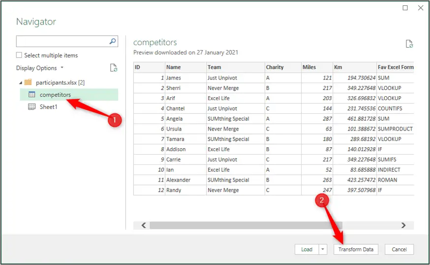
- In the Navigator window, select the competitors table and click Transform Data.
The Power Query Editor opens and shows a preview of the competitors table. We will not perform any transformations in this tutorial, except to create the data type.
Create a Power Query Data Type
You can include any columns you want in the data type. We will use all the columns.
- Click the ID column header, press and hold the Shift key and click the Pizza or Burger column header to select all the columns.
- Right click a column and click Create Data type, or click Transform > Create Data Type.
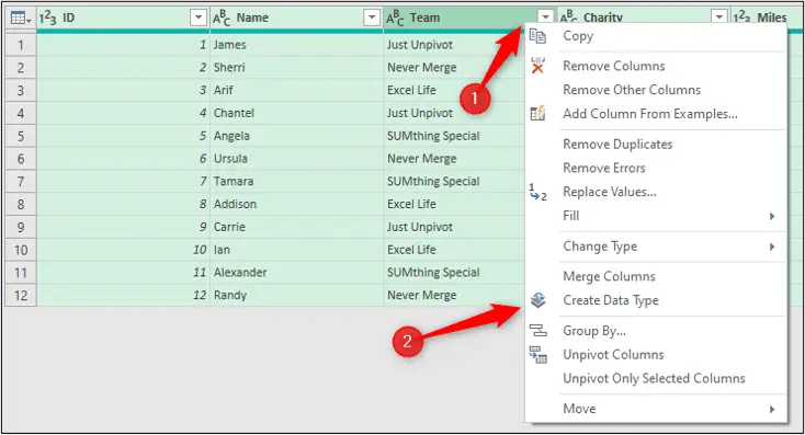
- In the Create Data Type window, type “Participants” for the Data type name and select Name from the list for the Display column. Click Ok.
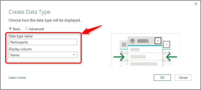
All the columns are combined into one record. You can see the custom data type icon in the column header.

- Click Home > Close & Load > Close & Load To.
- Select Table, Existing worksheet and load it to cell A1 of the competitors sheet.
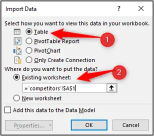
The custom data type is loaded to the worksheet. It is only one column wide so preserves space, yet is rich with data.
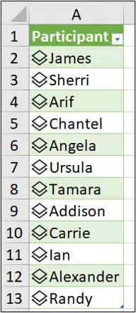
View the Data Type Columns
There are a few different ways to easily access the columns of a Power Query data type.
One simple way, is to click on the custom data type icon next to the names of the participants.
A pop up window shows the hidden columns. This includes the number of miles ran, the chosen charity and their favourite Excel formula.
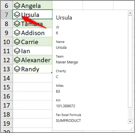
Another option is to display some of the columns physically on the worksheet.
Click the Add Column button next to the table header and click the column you want to add.
![]()
In this example, the Miles column has been added to the worksheet.
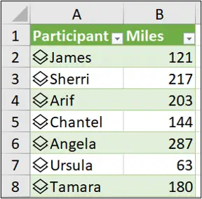
You can also add a column by typing the column name into the header row of the table.
In this example, the kilometres run is being added by typing the column header Km into an empty cell on the header row.
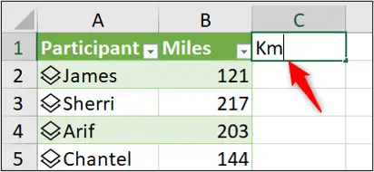
The typed header is matched to a custom data type header. Amazing!
You can also see the formula that was used to fetch this data.
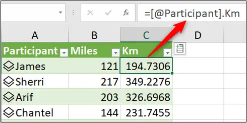
So, a final method would be to write a formula to add a column.
Type “=”, click the participant name and a list appears with the columns to choose from. Very easy.
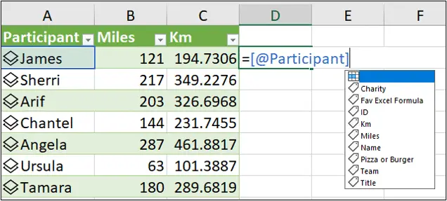
Formulas and Power Query Custom Data Types
Now, you do not need to add a column to the worksheet in order to use the columns from the data type. We can access them directly with formulas.
Let’s look at three examples of popular Excel formulas using the custom data type data.
We will start with a simple SUM function.
The following formula has been used in cell J2 of the dashboard to sum the total miles ran by all participants.
=SUM(competitors[Participants].Miles)
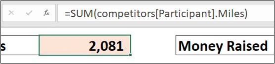
- Competitors – the name of the table
- Participant – the name of the data type column
- Miles – the name of the column within the data type that we want to use
Let’s take that a step further and use an XLOOKUP function to get data from the Power Query custom data type.
The following formula has been used in cell J4 to return the team that the winner (Angela in cell AH2) belonged to.
=XLOOKUP(AH2,competitors[Participant].Name,competitors[Participant].Team)

Finally, we will see an example of the FILTER function being used with the data type.
This example, is especially interesting because we will return the entire data type, not a single column of data.
The formula below has been used in cell E9 of the dashboard.
=SORTBY(
FILTER(competitors,competitors[Participant].Team=E8),
FILTER(competitors[Participant].Miles,competitors[Participant].Team=E8),
-1)
The array of the FILTER function is competitors. This returns the entire table and not just a specific column.
The SORTBY function is also used to order the data types by the number of miles ran.
You can see the data type icon next to the returned names in the image below. There is also the add column button to quickly insert additional columns if we wanted.
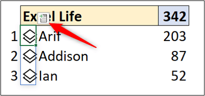
By returning the entire custom data type, we can quickly view extra information on our dashboard by clicking the data type icon.
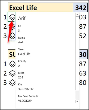
So, I hope this tutorial provided a nice over view of the Power Query custom data types and what they can offer.
I’m sure there are more exciting things to come in this space.