
My column headings are labeled with numbers instead of letters
- On the Excel menu, click Preferences.
- Under Authoring, click General .
- Clear the Use R1C1 reference style check box. The column headings now show A, B, and C, instead of 1, 2, 3, and so on.
Contents
- 1 How do you change Excel to Numbers?
- 2 How do I show column numbers in Excel?
- 3 How do I convert text to values in Excel?
- 4 How do I convert a column of numbers to column names in Excel?
- 5 How do I change the number format in Excel?
- 6 Why does Excel have numbers for columns?
- 7 How do I show columns and row numbers in Excel?
- 8 How do I get columns and row numbers in Excel?
- 9 How do I get row numbers in Excel?
- 10 How do I format numbers in Excel?
- 11 What are the different ways in formatting numbers?
- 12 How do I change the column title in Excel?
- 13 How do I change rows and column names in Excel?
- 14 How do I change Excel columns from numbers to alphabets?
- 15 How do I get rid of column 1 headers in Excel?
- 16 How do I change the row numbers in Excel?
- 17 What is an Xlookup in Excel?
- 18 Why can’t I see row numbers in Excel?
- 19 How do I add a numbered list in Excel?
- 20 How do I automatically number in sheets?
Change numbers with text format to number format in Excel for the…
- Select the cells that have the data you want to reformat.
- Click Number Format > Number. Tip: You can tell a number is formatted as text if it’s left-aligned in a cell.
How do I show column numbers in Excel?
Show column number
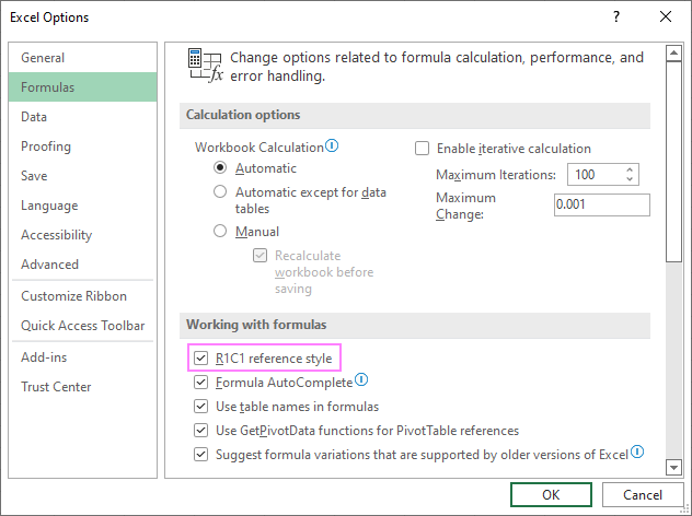
- Click File tab > Options.
- In the Excel Options dialog box, select Formulas and check R1C1 reference style.
- Click OK.
How do I convert text to values in Excel?
Use the Format Cells option to convert number to text in Excel
- Select the range with the numeric values you want to format as text.
- Right click on them and pick the Format Cells… option from the menu list. Tip. You can display the Format Cells…
- On the Format Cells window select Text under the Number tab and click OK.
How do I convert a column of numbers to column names in Excel?
To convert a column number to an Excel column letter (e.g. A, B, C, etc.) you can use a formula based on the ADDRESS and SUBSTITUTE functions. With this information, ADDRESS returns the text “A1”.
How do I change the number format in Excel?
You can use the Format Cells dialog to find the other available format codes:
- Press Ctrl+1 ( +1 on the Mac) to bring up the Format Cells dialog.
- Select the format you want from the Number tab.
- Select the Custom option,
- The format code you want is now shown in the Type box.
Why does Excel have numbers for columns?
Cause: The default cell reference style (A1), which refers to columns as letters and refers to rows as numbers, was changed. Solution: Clear the R1C1 reference style selection in Excel preferences. On the Excel menu, click Preferences.The column headings now show A, B, and C, instead of 1, 2, 3, and so on.
How do I show columns and row numbers in Excel?
On the Ribbon, click the Page Layout tab. In the Sheet Options group, under Headings, select the Print check box. , and then under Print, select the Row and column headings check box .
How do I get columns and row numbers in Excel?
It is quite easy to figure out the row number or column number if you know a cell’s address. If the cell address is NK60, it shows the row number is 60; and you can get the column with the formula of =Column(NK60). Of course you can get the row number with formula of =Row(NK60).
How do I get row numbers in Excel?
Use the ROW function to number rows
- In the first cell of the range that you want to number, type =ROW(A1). The ROW function returns the number of the row that you reference. For example, =ROW(A1) returns the number 1.
- Drag the fill handle. across the range that you want to fill.
How do I format numbers in Excel?
Formatting the Numbers in an Excel Text String
- Right-click any cell and select Format Cell.
- On the Number format tab, select the formatting you need.
- Select Custom from the Category list on the left of the Number Format dialog box.
- Copy the syntax found in the Type input box.
What are the different ways in formatting numbers?
How to change number formats. You can select standard number formats (General, Number, Currency, Accounting, Short Date, Long Date, Time, Percentage, Fraction, Scientific, Text) on the home tab of the ribbon using the Number Format menu. Note: As you enter data, Excel will sometimes change number formats automatically.
How do I change the column title in Excel?
Select a column, and then select Transform > Rename. You can also double-click the column header. Enter the new name.
How do I change rows and column names in Excel?
Rename columns and rows in a worksheet
- Click the row or column header you want to rename.
- Edit the column or row name between the last set of quotation marks. In the example above, you would overwrite the column name Gold Collection.
- Press Enter. The header updates.
How do I change Excel columns from numbers to alphabets?
To change the column headings to letters, select the File tab in the toolbar at the top of the screen and then click on Options at the bottom of the menu. When the Excel Options window appears, click on the Formulas option on the left. Then uncheck the option called “R1C1 reference style” and click on the OK button.
How do I get rid of column 1 headers in Excel?
Go to Table Tools > Design on the Ribbon. In the Table Style Options group, select the Header Row check box to hide or display the table headers. If you rename the header rows and then turn off the header row, the original values you input will be retained if you turn the header row back on.
How do I change the row numbers in Excel?
Here are the steps to use Fill Series to number rows in Excel:
- Enter 1 in cell A2.
- Go to the Home tab.
- In the Editing Group, click on the Fill drop-down.
- From the drop-down, select ‘Series..’.
- In the ‘Series’ dialog box, select ‘Columns’ in the ‘Series in’ options.
- Specify the Stop value.
- Click OK.
What is an Xlookup in Excel?
Use the XLOOKUP function to find things in a table or range by row.With XLOOKUP, you can look in one column for a search term, and return a result from the same row in another column, regardless of which side the return column is on.
Why can’t I see row numbers in Excel?
In order to show (or hide) the row and column numbers and letters go to the View ribbon. Set the check mark at “Headings”. That’s it!
How do I add a numbered list in Excel?
Click the Home tab in the Ribbon. Click the Bullets and Numbering option in the new group you created. The new group is on the far right side of the Home tab. In the Bullets and Numbering window, select the type of bulleted or numbered list you want to add to the text box and click OK.
How do I automatically number in sheets?
Use autofill to complete a series
- On your computer, open a spreadsheet in Google Sheets.
- In a column or row, enter text, numbers, or dates in at least two cells next to each other.
- Highlight the cells. You’ll see a small blue box in the lower right corner.
- Drag the blue box any number of cells down or across.
Содержание
- Columns and rows are labeled numerically in Excel
- Symptoms
- Cause
- Resolution
- More information
- A1 Reference Style vs. R1C1 Reference Style
- The A1 Reference Style
- The R1C1 Reference Style
- References
- What Are Columns In Excel?
- What are the rows and columns in Excel?
- What is column with example?
- What is row and column?
- What comes first row or column?
- What is row and?
- What are columns used for?
- What column means?
- How do I use columns in Excel?
- What is column in Table?
- Is a column across or down?
- What is Cell of MS Excel?
- What is the difference between row and column in a table?
- What is the matrix called?
- Why is Julia column-major?
- What is column article?
- How many column are there in Excel?
- How can you split a table?
- What are the 3 main parts of a column?
- Why are columns so strong?
- What is difference between column and columns in Excel?
- How to number columns in Excel and convert column letter to number
- How to return column number in Excel
- How to convert column letter to number (non-volatile formula)
- Change column letter to number using a custom function
- Return column number of a specific cell
- Get column letter of the current cell
- How to show column numbers in Excel
- How to number columns in Excel
Columns and rows are labeled numerically in Excel
Symptoms
Your column labels are numeric rather than alphabetic. For example, instead of seeing A, B, and C at the top of your worksheet columns, you see 1, 2, 3, and so on.
Cause
This behavior occurs when the R1C1 reference style check box is selected in the Options dialog box.
Resolution
To change this behavior, follow these steps:
- Start Microsoft Excel.
- On the Tools menu, click Options.
- Click the Formulas tab.
- Under Working with formulas, click to clear the R1C1 reference style check box (upper-left corner), and then click OK.
If you select the R1C1 reference style check box, Excel changes the reference style of both row and column headings, and cell references from the A1 style to the R1C1 style.
More information
A1 Reference Style vs. R1C1 Reference Style
The A1 Reference Style
By default, Excel uses the A1 reference style, which refers to columns as letters (A through IV, for a total of 256 columns), and refers to rows as numbers (1 through 65,536). These letters and numbers are called row and column headings. To refer to a cell, type the column letter followed by the row number. For example, D50 refers to the cell at the intersection of column D and row 50. To refer to a range of cells, type the reference for the cell that is in the upper-left corner of the range, type a colon (:), and then type the reference to the cell that is in the lower-right corner of the range.
The R1C1 Reference Style
Excel can also use the R1C1 reference style, in which both the rows and the columns on the worksheet are numbered. The R1C1 reference style is useful if you want to compute row and column positions in macros. In the R1C1 style, Excel indicates the location of a cell with an «R» followed by a row number and a «C» followed by a column number.
References
For more information about this topic, click Microsoft Excel Help on the Help menu, type about cell and range references in the Office Assistant or the Answer Wizard, and then click Search to view the topic.
Источник
What Are Columns In Excel?
In Microsoft Excel, a column runs vertically in the grid layout of a worksheet. Vertical columns are numbered with alphabetic values such as A, B, C. Horizontal rows are numbered with numeric values such 1, 2, 3.
What are the rows and columns in Excel?
Row and Column Basics
MS Excel is in tabular format consisting of rows and columns. Row runs horizontally while Column runs vertically. Each row is identified by row number, which runs vertically at the left side of the sheet. Each column is identified by column header, which runs horizontally at the top of the sheet.
What is column with example?
A column is a vertical series of cells in a chart, table, or spreadsheet. Below is an example of a Microsoft Excel spreadsheet with column headers (column letter) A, B, C, D, E, F, G, and H. As you can see in the image, the last column H is the highlighted column in red and the selected cell D8 is in the D column.
What is row and column?
A row is a series of data put out horizontally in a table or spreadsheet while a column is a vertical series of cells in a chart, table, or spreadsheet. Rows go across left to right. On the other hand, Columns are arranged from up to down.
What comes first row or column?
By convention, rows are listed first; and columns, second. Thus, we would say that the dimension (or order) of the above matrix is 3 x 4, meaning that it has 3 rows and 4 columns. Numbers that appear in the rows and columns of a matrix are called elements of the matrix.
What is row and?
1 : a number of objects arranged in a usually straight line a row of bottles also : the line along which such objects are arranged planted the corn in parallel rows. 2a : way, street.
What are columns used for?
Columns are frequently used to support beams or arches on which the upper parts of walls or ceilings rest. In architecture, “column” refers to such a structural element that also has certain proportional and decorative features.
What column means?
Definition of column
1a : a vertical arrangement of items printed or written on a page columns of numbers. b : one of two or more vertical sections of a printed page separated by a rule or blank space The news article takes up three columns. c : an accumulation arranged vertically : stack columns of paint cans.
How do I use columns in Excel?
To insert columns:
- Select the column heading to the right of where you want the new column to appear. For example, if you want to insert a column between columns D and E, select column E.
- Click the Insert command on the Home tab. Clicking the Insert command.
- The new column will appear to the left of the selected column.
What is column in Table?
A column is collection of cells aligned vertically in a table. A field is an element in which one piece of information is stored, such as the eceived field. Usually, a column in a table contains the values of a single field.
Is a column across or down?
Columns run vertically, up and down.Rows, then, are the opposite of columns and run horizontally.
What is Cell of MS Excel?
Cells are the boxes you see in the grid of an Excel worksheet, like this one. Each cell is identified on a worksheet by its reference, the column letter and row number that intersect at the cell’s location. This cell is in column D and row 5, so it is cell D5. The column always comes first in a cell reference.
What is the difference between row and column in a table?
Rows are a group of cells arranged horizontally to provide uniformity. Columns are a group of cells aligned vertically, and they run from top to bottom.
What is the matrix called?
A matrix (whose plural is matrices) is a rectangular array of numbers, symbols, or expressions, arranged in rows and columns. A matrix with m rows and n columns is called an m×n m × n matrix or m -by-n matrix, where m and n are called the matrix dimensions.
Why is Julia column-major?
Probably because most numeric libraries were originally written in Fortran, which uses column-major storage, which then mimics the fact that vectors in math are by convention columns. Same applies to Matlab, which started as a convenient way to speak to some Fortran linear algebra packages.
What is column article?
A column is a recurring piece or article in a newspaper, magazine or other publication, where a writer expresses their own opinion in few columns allotted to them by the newspaper organisation. Columns are written by columnists.
How many column are there in Excel?
Worksheet and workbook specifications and limits
| Feature | Maximum limit |
|---|---|
| Open workbooks | Limited by available memory and system resources |
| Total number of rows and columns on a worksheet | 1,048,576 rows by 16,384 columns |
| Column width | 255 characters |
| Row height | 409 points |
How can you split a table?
Split a table
- Put your cursor on the row that you want as the first row of your second table. In the example table, it’s on the third row.
- On the LAYOUT tab, in the Merge group, click Split Table. The table splits into two tables.
What are the 3 main parts of a column?
Classical columns traditionally have three main parts:
- The base. Most columns (except the early Doric) rest on a round or square base, sometimes called a plinth.
- The shaft. The main part of the column, the shaft, may be smooth, fluted (grooved), or carved with designs.
- The capital.
Why are columns so strong?
Columns are vertical structural members designed to pass through a compressive load.Engineers have to design columns that are very strong under compression in order to keep buildings safe.
What is difference between column and columns in Excel?
Each row has a unique number that identifies it. A column is a vertical line of cells. Each column has a unique letter that identifies it.
Comparative Table.
Источник
How to number columns in Excel and convert column letter to number
 by Svetlana Cheusheva, updated on March 9, 2023
The tutorial talks about how to return a column number in Excel using formulas and how to number columns automatically.
Last week, we discussed the most effective formulas to change column number to alphabet. If you have an opposite task to perform, below are the best techniques to convert a column name to number.
How to return column number in Excel
To convert a column letter to column number in Excel, you can use this generic formula:
For example, to get the number of column F, the formula is:
And here’s how you can identify column numbers by letters input in predefined cells (A2 through A7 in our case):
Enter the above formula in B2, drag it down to the other cells in the column, and you will get this result: 
How this formula works:
First, you construct a text string representing a cell reference. For this, you concatenate a letter and number 1. Then, you hand off the string to the INDIRECT function to convert it into an actual Excel reference. Finally, you pass the reference to the COLUMN function to get the column number.
How to convert column letter to number (non-volatile formula)
Being a volatile function, INDIRECT can significantly slow down your Excel if used broadly in a workbook. To avoid this, you can identify the column number using a slightly more complex non-volatile alternative:
This works perfectly in dynamic array Excel (365 and 2021). In older version, you need to enter it as an array formula (Ctrl + Shift + Enter) to get it to work.
=MATCH(A2&»1″, ADDRESS(1, COLUMN($1:$1), 4), 0)
Or you can use this non-array formula in all Excel versions:
=MATCH(A2&»1″, INDEX(ADDRESS(1, INDEX(COLUMN($1:$1), ), 4), ), 0) 
How this formula works:
First off, you concatenate the letter in A2 and the row number «1» to construct a standard «A1» style reference. In this example, we have letter «A» in A2, so the resulting string is «A1».
Next, you get an array of strings representing all cell addresses in the first row, from «A1» to «XFD1». For this, you use the COLUMN($1:$1) function, which generates a sequence of column numbers, and pass that array to the column_num argument of the ADDRESS function:
Given that row_num (1st argument) is set to 1 and abs_num (3rd argument) is set to 4 (meaning you want a relative reference), the ADDRESS function delivers this array:
Finally, you build a MATCH formula that searches for the concatenated string in the above array and returns the position of the found value, which corresponds to the column number you are looking for:
Change column letter to number using a custom function
«Simplicity is the ultimate sophistication,» stated the great artist and scientist Leonardo da Vinci. To get a column number from a letter in an easy way, you can create your own custom function.
Fully in line with the above principle, the function’s code is as simple as it can possibly be:
Insert the code in your VBA editor as explained here, and your new function named ColumnNumber is ready for use.
The function requires just one argument, col_letter, which is the column letter to be converted into a number:
Your real formula can be as follows:
If you compare the results returned by our custom function and Excel’s native ones, you will make sure they are exactly the same: 
Return column number of a specific cell
To get a column number of a particular cell, simply use the COLUMN function:
For instance, to identify the column number of cell B3, the formula is:
Obviously, the result is 2. 
Get column letter of the current cell
To find out a column number of the current cell, use the COLUMN() function with an empty argument, so it refers to the cell where the formula is:
=COLUMN() 
How to show column numbers in Excel
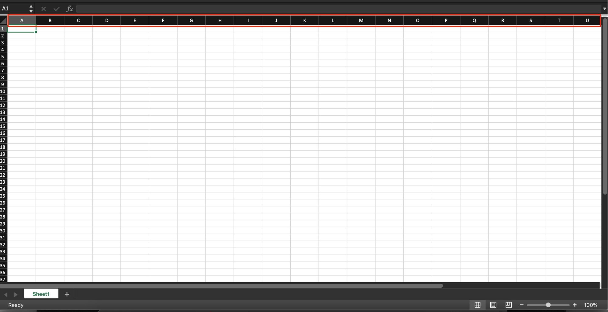
By default, Excel uses the A1 reference style and labels column headings with letters and rows with numbers. To get columns labeled with numbers, change the default reference style from A1 to R1C1. Here’s how:
- In your Excel, click File >Options.
- In the Excel Options dialog box, select Formulas in the left pane.
- Under Working with formulas, check the R1C1 reference style box, and click OK.

The column labels will immediately change from letters to numbers: 
Please note that selecting this option will not only change column labels — cell addresses will also change from A1 to R1C1 references, where R means «row» and C means «column». For example, R1C1 refers to the cell in row 1 column 1, which corresponds to the A1 reference. R2C3 refers to the cell in row 2 column 3, which corresponds to the C2 reference.
In existing formulas, cell references will update automatically, while in new formulas you will have to use the R1C1 reference style.
Tip. To revert back to A1 style, uncheck the R1C1 reference style check box in Excel Options.
How to number columns in Excel
If you are not used to the R1C1 reference style and want to keep A1 references in your formulas, then you can insert numbers in the first row of our worksheet, so you have both — column letters and numbers. This can be easily done with the help of the Auto Fill feature.
Here are the detailed steps:
- In A1, type number 1.
- In B1, type number 2.
- Select cells A1 and B1.
- Hover the cursor over a small square in the lower right corner of cell B1, which is called the Fill handle. As you do this, the cursor will change to a thick black cross.
- Drag the fill handle to the right up to the column you need.

As a result, you will retain the column labels as letters, and underneath the letters you will have the column numbers.
Tip. To keep the columns numbers in view while scrolling to the below areas of the worksheet, you can freeze top row.
That’s how to return column numbers in Excel. I thank you for reading and look forward to seeing you on our blog next week!
Источник
Last Update: Jan 03, 2023
This is a question our experts keep getting from time to time. Now, we have got the complete detailed explanation and answer for everyone, who is interested!
Asked by: Ethan Leffler
Score: 4.2/5
(69 votes)
By default, Excel uses the A1 reference style, which refers to columns as letters (A through IV, for a total of 256 columns), and refers to rows as numbers (1 through 65,536). These letters and numbers are called row and column headings. To refer to a cell, type the column letter followed by the row number.
What are columns Labelled as in Excel?
By default, Excel uses the A1 reference style, which refers to columns as letters (A through IV, for a total of 256 columns), and refers to rows as numbers (1 through 65,536). These letters and numbers are called row and column headings. To refer to a cell, type the column letter followed by the row number.
What are columns identified by in Excel?
Columns are identified by letters (A, B, C), while rows are identified by numbers (1, 2, 3). Each cell has its own name—or cell address—based on its column and row.
Why Excel columns are numbers?
Cause: The default cell reference style (A1), which refers to columns as letters and refers to rows as numbers, was changed. Solution: Clear the R1C1 reference style selection in Excel preferences. On the Excel menu, click Preferences. … The column headings now show A, B, and C, instead of 1, 2, 3, and so on.
Which is not a function in MS Excel?
The correct answer to the question “Which one is not a function in MS Excel” is option (b). AVG. There is no function in Excel like AVG, at the time of writing, but if you mean Average, then the syntax for it is also AVERAGE and not AVG. The other two options are correct.
40 related questions found
Where is authoring in Excel?
With the file still open in Excel, make sure that AutoSave is on in the upper-left corner. When others eventually open the file, you’ll be co-authoring together. You know you’re co-authoring if you see pictures of people in the upper-right of the Excel window.
What are the columns and rows in Excel?
Key Differences
- Rows are the horizontal lines in the worksheet, and columns are the vertical lines in the worksheet.
- In the worksheet, the total rows are 10,48,576, while the total columns are 16,384.
- In the worksheet, rows are ranging from 1 to 1,048,576, while columns are ranging from A to XFD.
What is the difference between rows and columns in Excel?
Rows are a group of cells arranged horizontally to provide uniformity. Columns are a group of cells aligned vertically, and they run from top to bottom.
How do I calculate rows and columns in Excel?
If you need to sum a column or row of numbers, let Excel do the math for you. Select a cell next to the numbers you want to sum, click AutoSum on the Home tab, press Enter, and you’re done. When you click AutoSum, Excel automatically enters a formula (that uses the SUM function) to sum the numbers.
How do I make labels from columns in Excel?
- Type in a heading in the first cell of each column describing the data. Make a column for each element you want to include on the labels. Lifewire.
- Type the names and addresses or other data you’re planning to print on labels. Make sure each item is in the correct column. …
- Save the worksheet when you have finished.
What are toolbars in Excel?
Excel toolbar (also called Quick Access Toolbar. It enables users to save important shortcuts and easily access them when needed. read more) is presented to get access to various commands to perform the operations. It is presented with an option to add or delete commands to it to access them quickly.
Can’t see rows and column numbers Excel?
Step 1 — Click on «View» Tab on Excel Ribbon. Step 3 — Uncheck «Headings» checkbox to hide Excel worksheet Row and Column headings. Check «Headings» checkbox to show missing hidden Excel worksheet Row and Column headings, as explained in below image.
What is called row and column?
The vertical arrangement of objects on the basis of a category is called a column. When the objects are arranged in a horizontal manner, it is referred to as a row. … Rows are records that contain fields in DBMS. Vertical arrays in a matrix are called columns. Horizontal arrays are called rows in matrix.
What is column in Excel?
In Microsoft Excel, a column runs vertically in the grid layout of a worksheet. Vertical columns are numbered with alphabetic values such as A, B, C. … Each column in the worksheet has its own column number which is used as part of a cell reference such as A1, A2, or M16.
What is the shortcut to convert rows to columns in Excel?
How to use the macro to convert row to column
- Open the target worksheet, press Alt + F8, select the TransposeColumnsRows macro, and click Run.
- Select the range that you want to transpose and click OK:
- Select the upper left cell of the destination range and click OK:
How do I convert multiple columns to rows in Excel?
Highlight all of the columns that you want to unpivot into rows, then click on Unpivot Columns just above your data. Once you’ve clicked on Unpivot Columns, Excel will transform your columnar data into rows. Each row is a record of its own, ready to throw into a Pivot Table or work with in your datasheet.
How do you identify rows and columns?
A row is a series of data put out horizontally in a table or spreadsheet while a column is a vertical series of cells in a chart, table, or spreadsheet. Rows go across left to right. On the other hand, Columns are arranged from up to down.
Where is the Editing tab in Excel?
Click File > Options > Advanced. , click Excel Options, and then click the Advanced category. Under Editing options, do one of the following: To enable Edit mode, select the Allow editing directly in cells check box.
Where is preferences in Excel?
Choose Excel→Preferences from the menu bar to display the Preferences dialog.
How do I turn on AutoSave in Excel?
How to Turn on AutoSave in Excel
- Open Excel and select File > Options.
- In the menu that opens, select Save on the left.
- If you have a OneDrive or SharePoint account, select AutoSave OneDrive and SharePoint Online files by default on Excel.
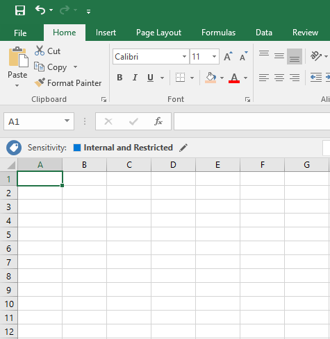
Have you ever opened an Excel workbook and found that the column headings show numbers instead of letters? The formula look strange too, showing references like RC[-1] instead of D2.

This is R1C1 reference style — a handy feature, and I use it sometimes when programming or setting up a workbook.
Numbers on the column headings make it easier to set up formulas that need a column number, such as VLOOKUP. I don’t have to get fingerprints on my screen, as I count across to column R, where the lookup value is.
Video: Change Excel Column Headings from Numbers to Letters
To see why this happens, and how to switch the column headings back to letters, watch this short video tutorial. The written instructions are below the video.
Your browser can’t show this frame. Here is a link to the page
Why It Happens
Maybe you’ve never heard of R1C1 reference style, and certainly didn’t change any settings. If you didn’t turn that option on, why did the numbers suddenly appear? Probably because someone sent you a workbook, and that’s the first Excel file that you opened today.
The first workbook that you open, when opening Excel, sets the reference style. For example, perhaps I built a workbook for you, and saved it while I was using R1C1 reference style.
I sent you the workbook overnight, and it was the first thing you opened this morning. Surprise! There are numbers in the column headings.
Turn R1C1 Reference Style On or Off
If you close Excel, then open a workbook that you created yourself, with letters in the column headings, that will change the reference style back to A1, which has letters in the column headings.
Or, to manually change the reference style, you can change the option setting.
In Excel 2010:
- At the left end of the Ribbon, click the File tab, then click Options.
- Click the Formulas category.
- In the Working with Formulas section, add or remove the check mark from ‘R1C1 reference style’
- Click OK to close the Options window.

In Excel 2007:
-
- At the left end of the Ribbon, click the Office Button, then click Excel Options.
- Click the Formulas category.
- In the Working with Formulas section, add or remove the check mark from ‘R1C1 reference style’
- Click OK to close the Options window.
In Excel 2003 and earlier versions:
- On the Tools menu, click Options and select the General tab.
- Add or remove the check mark from ‘R1C1 reference style’
- Click OK to close the Options dialog box.

Use a Macro to Switch Headings
If you frequently change the headings from numbers to letters, or letters to numbers, you can create a macro to do the work for you.
There are instructions in this blog post: Excel VBA: Switch Column Headings to Numbers
________________________

Microsoft Excel displays data in tabular format. This means that information is arranged in a table consisting of rows and columns.
Rows and columns are different properties that together make up a table.
These are the two most important features of Excel that allow users to store and manipulate their data.
Below we’ll discuss the definitions of a row and a column, along with the differences between these two features.
Each row is denoted and identified by a unique numeric value that you’ll see on the left hand side.
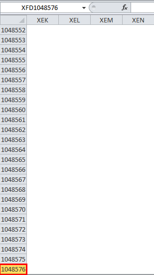
The row numbers are arranged vertically on the worksheet, ranging from 1-1,048,576 (you can have a total of 1,048,576 rows in Excel).
The rows themselves run horizontally on a worksheet.
Data is placed horizontally in the table, and goes across from left to right.
Row 1 is the first row in Excel.
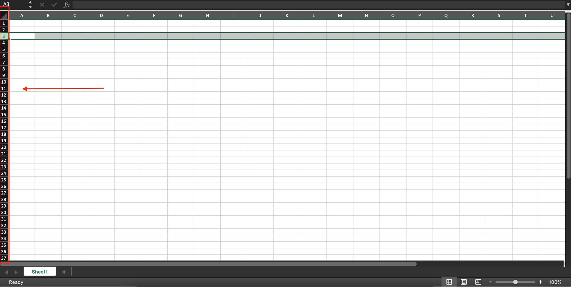
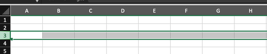
As you can see in the example below, you can select the whole row with the number 3 by clicking on the number itself.
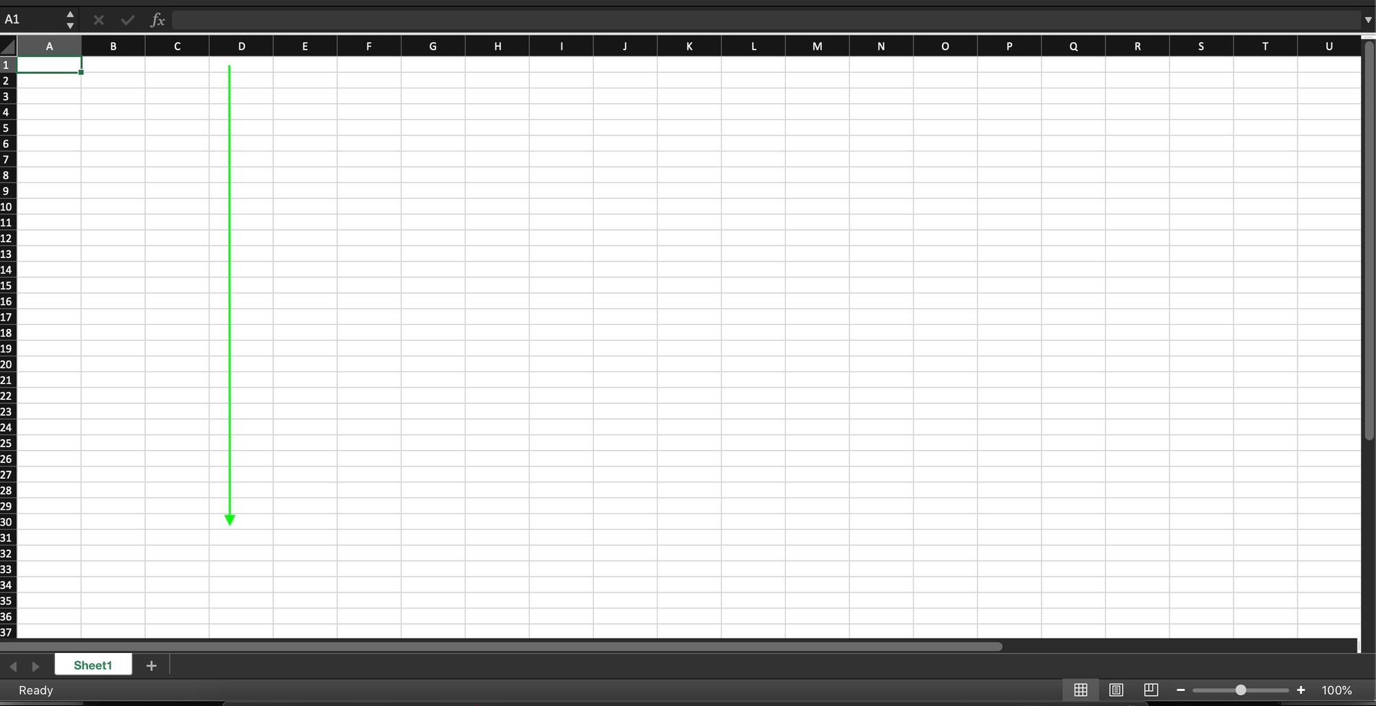
To navigate through the numbers and reach the last row, you can use:
- For Windows Users:
Control down navigation arrow. You first press the Control key and then, while holding it down, press the down navigation arrow. - For Mac Users:
Command down navigation arrow. You first press the Command key and then, while holding it down, press the down navigation arrow.
To get back to the first row (the top) again, press Control up navigation arrow for Windows and Command up navigation arrow for Mac.
What is a column in Excel?
Columns are denoted and identified by a unique alphabetical header letter, which is located at the top of the worksheet.
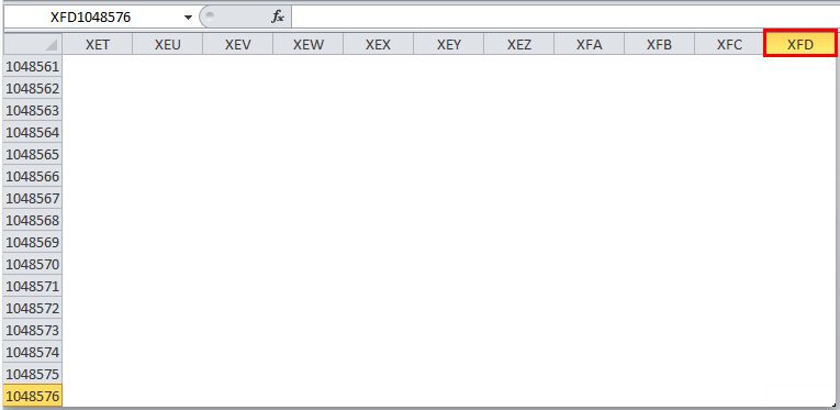
Column headers range from A-XFD, as Excel spreadsheets can have 16,384 columns in total.
Columns run vertically in the worksheet, and the data goes from up to down.
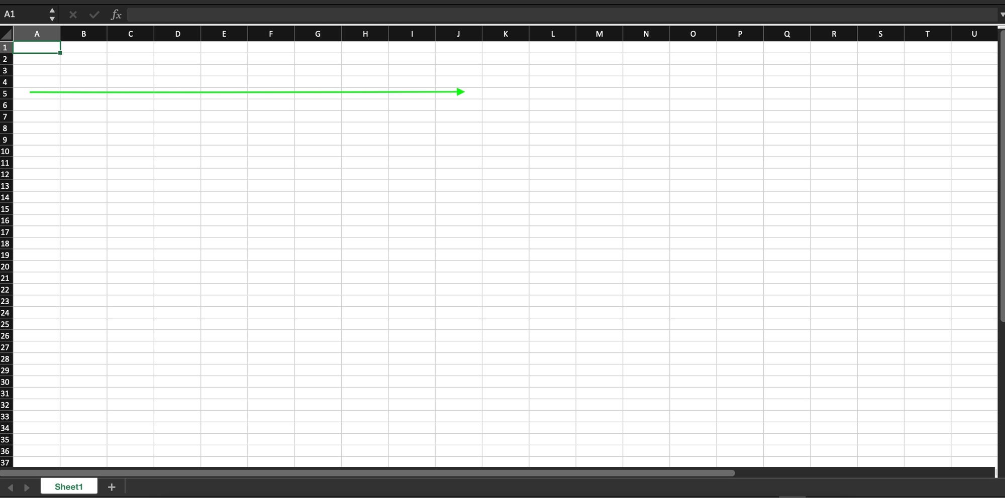
Column A is the first column in Excel.
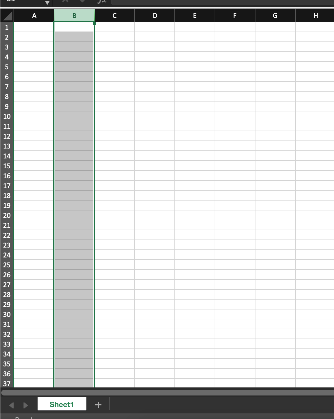
In the example below, you can see that the whole column with header B is selected by pressing/clicking on the letter at the top.
To move to the last column:
- For Windows Users:
Control right navigation arrow. First press the Control key and then, while holding it down, press the right navigation arrow. - For Mac Users:
Command right navigation arrow. First press the Command key and then, while holding it down, press the right navigation arrow.
To get back to the first column again, press Control left navigation arrow for Windows and Command left navigation arrow for Mac.
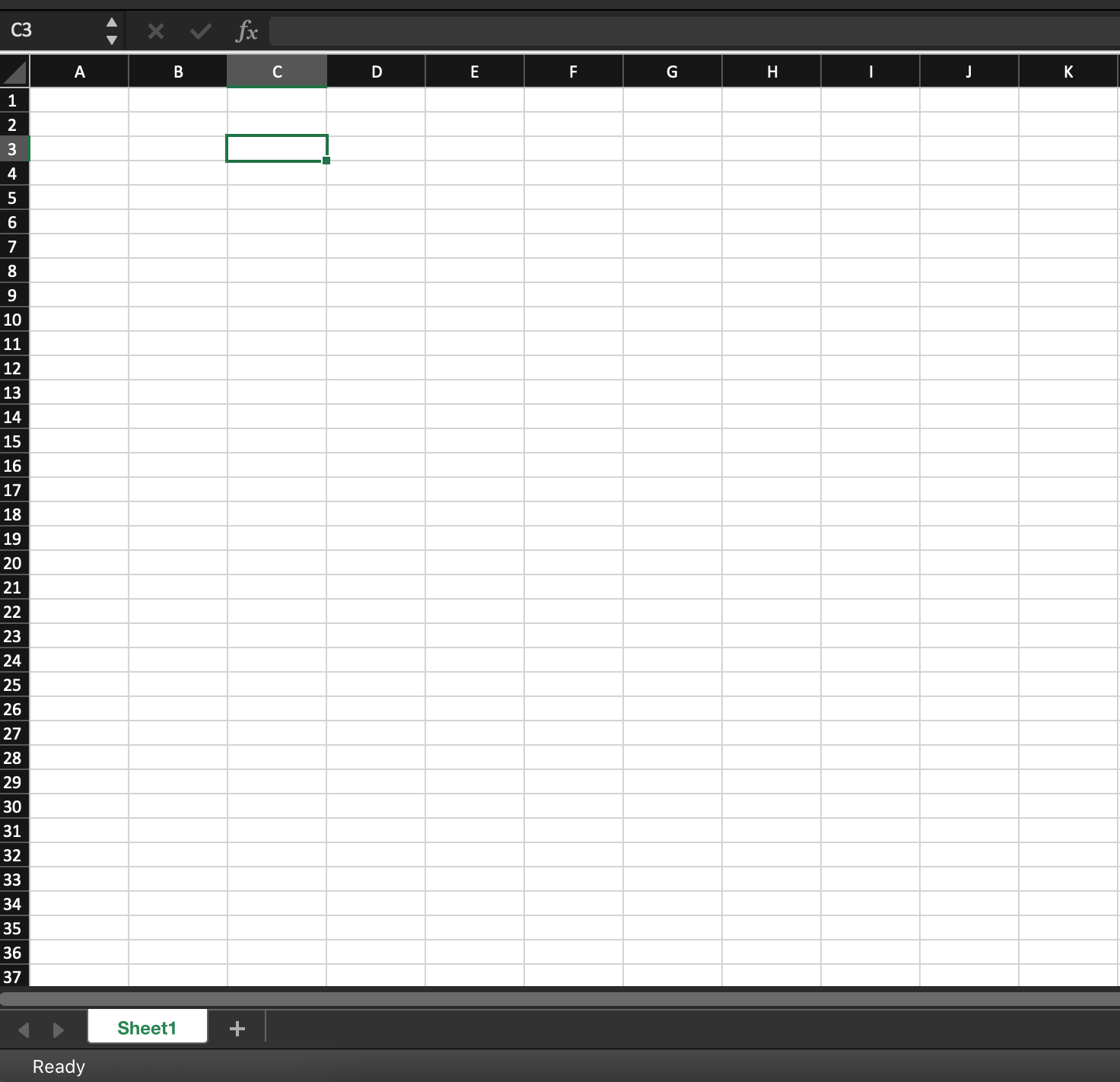
What is a cell in Excel?
A cell is the intersection of a row and a column. A row and a column adjoined make up a cell.
You can define a cell by the combination of a row number and a column header.
For example, below the selected cell is C3. It has a column header C and a row number 3.
We can also select an entire row or column from a cell.
To select the whole row when in any cell, press Shift Space.
To select the whole column when in any cell, press Ctrl Space.
Conclusion
Now you know the definitions of rows and columns in Excel. You’ve learned their main differences and how they work.
In summary, information in a row is presented horizontally, whereas in a column information is vertical.
Thanks for reading!
Learn to code for free. freeCodeCamp’s open source curriculum has helped more than 40,000 people get jobs as developers. Get started
Difference Between Excel Rows and Columns
Rows and columns are two different properties in Excel that make up a cell, range, or table together. In general terms, the vertical portion of the Excel worksheet is known as columns. For example, there can be 256 of them in a worksheet. The horizontal portion of the worksheet is known as rows. For example, there can be 1,048,576 of them.
Excel is the cobweb of rows and columns. Each adjacent row and column is termed a cell. A worksheet consists of millions of such cells that can gather and record its data. The main aim of using Excel is to plot the data in it as per the requirement and manipulate the same to obtain a fruitful analysis.
Table of contents
- Difference Between Excel Rows and Columns
- Excel Rows vs Columns Infographics
- Key Differences
- Comparative Table
- Conclusion
- Recommended Articles
- Excel rows and columns are two different characteristics that combine to create a table or cell.
- Millions of these cells comprise a worksheet, which may collect and store data. Excel is mostly used to plot data according to specifications and edit that data to produce insightful analyses.
- Rows represent numerical value, whereas columns represent alphabets.
- On average, there are a total number of 1,048,576 rows and 16,384 numbers of columns.
The corporates have high dependability on Excel to perform their day-to-day business decisions and run their daily operations. This article will discuss the top differences between excel rows and columnsA cell is the intersection of rows and columns. Rows and columns make the software that is called excel. The area of excel worksheet is divided into rows and columns and at any point in time, if we want to refer a particular location of this area, we need to refer a cell.read more.
- A row is a horizontal line of cells. Each row has a unique number that identifies it.
- A column is a vertical line of cells. Each column has a special letter that identifies it.
Let us understand this with an example:
The leftmost column is A, and the next column is B. In addition, the topmost row is 1, and the next row is 2. The adjacent top row creates the cell, and the leftmost Column is A1, as reflected in the figure.
Excel Rows vs Columns Infographics
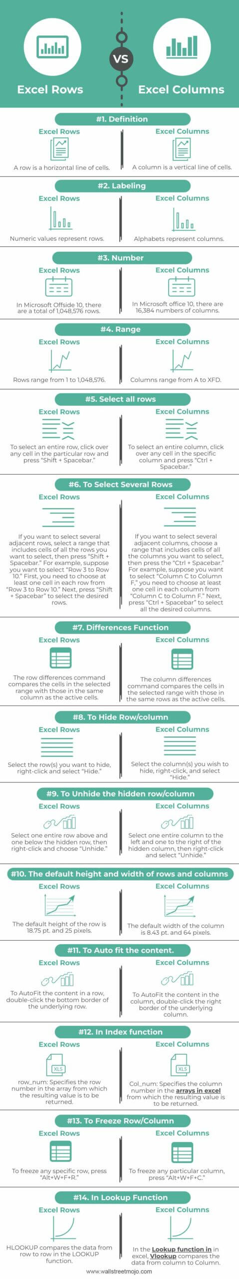
Key Differences
- Rows are the horizontal lines in the worksheet, and columns are the vertical lines in the worksheet.
- In the worksheet, the total rows are 10,48,576, while the total columns are 16,384.
- In the worksheet, rows range from 1 to 1,048,576, while columns range from A to XFD.
- To select an entire specific row, press “Shift + Spacebar.” To select the whole column, press “Ctrl+ Spacebar.”
- To hide any row, select the entire row and press right click and then hide, while to hide any column in excelThe methods to hide columns in excel are — hide columns using right-click option, hide columns using shortcut cut key, hide columns using column width, hide columns using VBA code.read more, select the whole column, press right-click, and then “Hide.”
- To unhide any hidden row, select one entire row above and one below the hidden row, then right-click and choose “Unhide.” To unhide any hidden excel columnUsing the Home tab of the Excel ribbon, using the shortcut key, using the context menu, altering the column width, using the ctrl+G (go to) command, and using the ctrl+F (find) command are some of the ways to unhide a column in Excel.read more, choose one entire column to the left and one to the right of the hidden column, then right-click and select “Unhide.”
- The default row height is 18.75 pt. and 25 pixels, while the default width of the column is 8.43 pt. and 64 pixels.
- To freeze any row, put the active cell below the row one wants to freeze and then press “Alt+W+F+R.” To freeze any column, set the active cell adjacent to the column one wants to freeze, and then press “Alt+W+F+C.”
Comparative Table
| Basis | Excel Rows | Excel Columns |
|---|---|---|
| Definition | A row is a horizontal line of cells. | A column is a vertical line of cells. |
| Labeling | Numeric values represent rows. | Alphabets represent columns. |
| Number | In Microsoft Offside 10, there are a total of 1,048,576 rows. | In Microsoft office 10, there are 16,384 numbers of columns. |
| Range | Rows range from 1 to 1,048,576. | Columns range from A to XFD. |
| Select all rows | To select an entire row, click over any cell in the particular row and press “Shift + Spacebar.” | To select an entire column, click over any cell in the specific column and press “Ctrl + Spacebar.” |
| To Select Several Rows | If you want to select several adjacent rows, select a range that includes cells of all the rows you want to select, then press “Shift + Spacebar.” For example, suppose you want to select “Row 3 to Row 10.” First, you need to choose at least one cell in each row from “Row 3 to Row 10.” Next, press “Shift + Spacebar” to select the desired rows. | If you want to select several adjacent columns, choose a range that includes cells of all the columns you want to select, then press the “Ctrl + Spacebar.” For example, suppose you want to select “Column C to Column F,” you need to choose at least one cell in each column from “Column C to Column F.” Next, press “Ctrl + Spacebar” to select all the desired columns. |
| Differences Function | The row differences command compares the cells in the selected range with those in the same column as the active cells. | The column differences command compares the cells in the selected range with those in the same rows as the active cells. |
| To Hide Row/column | Select the row(s) you want to hide, right-click and select “Hide.” | Select the column(s) you wish to hide, right-click, and select “Hide.” |
| To Unhide the hidden row/column | Select one entire row above and one below the hidden row, then right-click and choose “Unhide.” | Select one entire column to the left and one to the right of the hidden column, then right-click and select “Unhide.” |
| The default height and width of rows and columns | The default height of the row is 18.75 pt. and 25 pixels. | The default width of the column is 8.43 pt. and 64 pixels. |
| To Auto fit the content. | To AutoFit the content in a row, double-click the bottom border of the underlying row. | To AutoFit the content in the column, double-click the right border of the underlying column. |
| In Index functionThe INDEX function in Excel helps extract the value of a cell, which is within a specified array (range) and, at the intersection of the stated row and column numbers.read more | row_num: Specifies the row number in the array from which the resulting value is to be returned. | Col_num: Specifies the column number in the arrays in excelArray formulas are extremely helpful and powerful formulas that are used in Excel to execute some of the most complex calculations. There are two types of array formulas: one that returns a single result and the other that returns multiple results.read more from which the resulting value is to be returned. |
| To Freeze Row/Column | To freeze any specific row, press “Alt+W+F+R.” | To freeze any particular column, press “Alt+W+F+C.” |
| In Lookup Function | HLOOKUP compares the data from row to row in the LOOKUP function. | In the Lookup function inThe LOOKUP excel function searches a value in a range (single row or single column) and returns a corresponding match from the same position of another range (single row or single column). The corresponding match is a piece of information associated with the value being searched. read more in excel, VlookupThe VLOOKUP excel function searches for a particular value and returns a corresponding match based on a unique identifier. A unique identifier is uniquely associated with all the records of the database. For instance, employee ID, student roll number, customer contact number, seller email address, etc., are unique identifiers. read more compares the data from column to Column. |
Conclusion
Excel spreadsheets have huge potential based on the data feed in the rows and columns. And accordingly, the same is utilized in various functions in the corporate world. Moreover, users prepare several data models based on the requirements that give them automated results and enhance analytical skills.
Recommended Articles
This article is a guide to Excel Rows vs. Columns. We discuss the top differences between Excel rows, columns, infographics, and a comparison table. You may also look at the following articles: –
- Excel vs. Google Sheets – Compare
- Excel vs. Access
- VLOOKUP with Two Criteria
- What is Database in Excel?
Reader Interactions

This Excel tutorial explains how to change column headings from numbers (1, 2, 3, 4) back to letters (A, B, C, D) in Excel 2016 (with screenshots and step-by-step instructions).
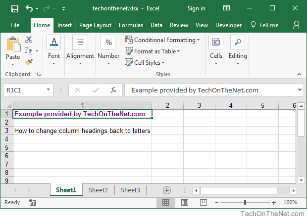
Question: In Microsoft Excel 2016, my Excel spreadsheet has numbers for both rows and columns. How do I change the column headings back to letters such as A, B, C, D?
Answer: Traditionally, column headings are represented by letters such as A, B, C, D. If your spreadsheet shows the columns as numbers, you can change the headings back to letters with a few easy steps.
In the example below, the column headings are numbered 1, 2, 3, 4 instead of the traditional A, B, C, D values that you normally see in Excel. When the column headings are numeric values, R1C1 reference style is being displayed in the spreadsheet.
To change the column headings to letters, select the File tab in the toolbar at the top of the screen and then click on Options at the bottom of the menu.
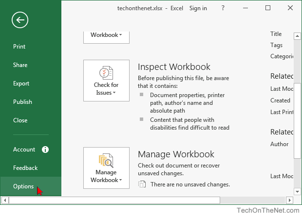
When the Excel Options window appears, click on the Formulas option on the left. Then uncheck the option called «R1C1 reference style» and click on the OK button.

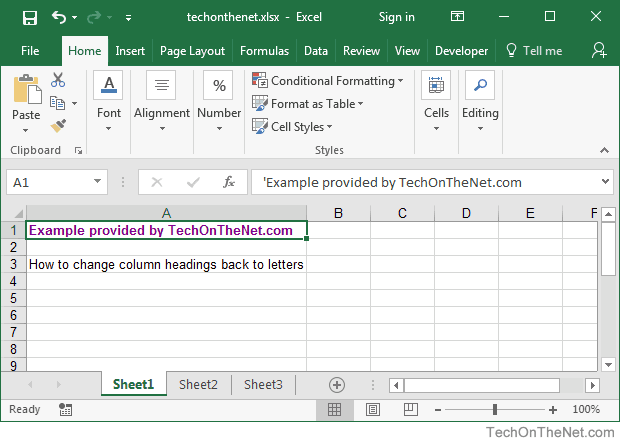
Now when you return to your spreadsheet, the column headings should be letters (A, B, C, D) instead of numbers (1, 2, 3, 4).
Rows and Column in Excel (Table of Contents)
- Introduction to Rows and Column in Excel
- Rows and Column Navigation in excel
- How to Select Rows and Column in excel?
- Adjusting Column Width
Introduction to Rows and Column in Excel
In Microsoft excel, if we open a new workbook, we can see that sheet will contain tables with light grey color. Basically excel is a tabular format which contains n number of rows and columns, where rows in excel will be in a horizontal line, and column in excel will be in a vertical line.
- In excel, we can find each row by its row number, which is shown in the below screenshot, which shows vertical numbers on the left side of each sheet.
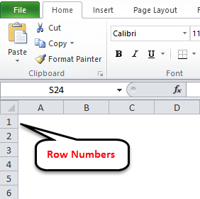
- As we can see in the above screenshot that each row can be identified by their row numbers like 1, 2, 3 etc.
- Whereas we can find the column in excel, which can be identified by the column header like A, B, C. which will be shown normally in all excel sheets, which are shown below.
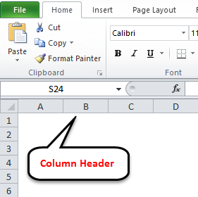
- In Excel, each column is named by its header, which shows the column header horizontally at the top of the excel sheet.
In Microsoft Excel 2010 and the latest version, we have row numbers ranging from 1 to 1048576 in 1048576, whereas the column ranges from A to XFD in a total of 16384 columns which is shown in the below screenshot.
Rows in excel range from 1 to 1048576, which is highlighted in red mark
The column in excel ranges from A to XFD, which is highlighted in red mark.
Rows and Column Navigation in excel
In this example, we will see how to navigate rows and columns with the below examples.
We can find the last row of excel by using the keyboard shortcut key CTRL+DOWN NAVIGATION ARROW KEY, or else we can use the vertical scrollbars to go to the end of the row.
We can find the last column of excel by using the CTRL+RIGHT NAVIGATION ARROW KEY, or else we can use the horizontal scrollbars to go to the end of the column.
How to Select Rows and Column in excel?
In this example, we will learn how to select the rows and columns in excel.
You can download this Rows and Column Excel Template here – Rows and Column Excel Template
Rows and Column in Excel – Example#1
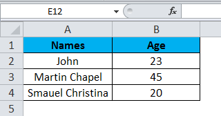
Normally, when we open a workbook, we can see that sheet contains tabular rows and columns where each row is specified by their row number and column specified by their column header.
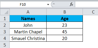
Consider the below example, which has some data in an excel sheet. Here we will see how to select the rows and columns.
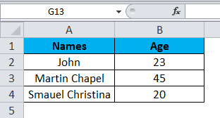
In the above screenshot, we can see that names and age column have their own header name A and B, and each row has its own row number.
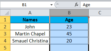
In excel, each time when we select a row or column, “Name Box” will display the specific row number and column name, which is shown in the below screenshot.
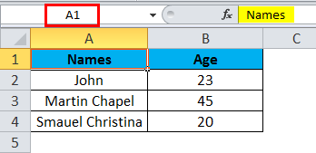
In this example, we will select the Names and Age, and let’s see how the rows and column header is getting displayed.
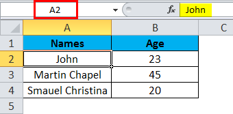
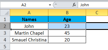
Step 1 – First, select the cell Name John.
Step 2 – Once you select the cell name, John, we will get the row number and column name as A2 in the name box, which means that we have selected A column second row as A2, shown below screenshot with yellow highlighted.
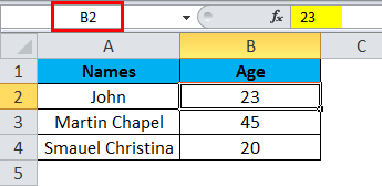
Step 3 – Now select cell 23, where it will show the selected cell is B2 which is shown in the below screenshot with yellow highlighted.
Step 4 – Now select all the names and columns to show that we have 4 rows and 2 columns shown in the below screenshot.
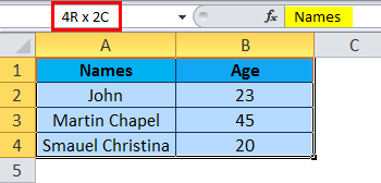
In this way, we can identify the row number and column name by selecting each cell in excel.
Example#2 – Changing Row and Column Size
This example shows how to change the row and column size by using the following examples.
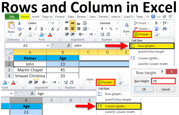
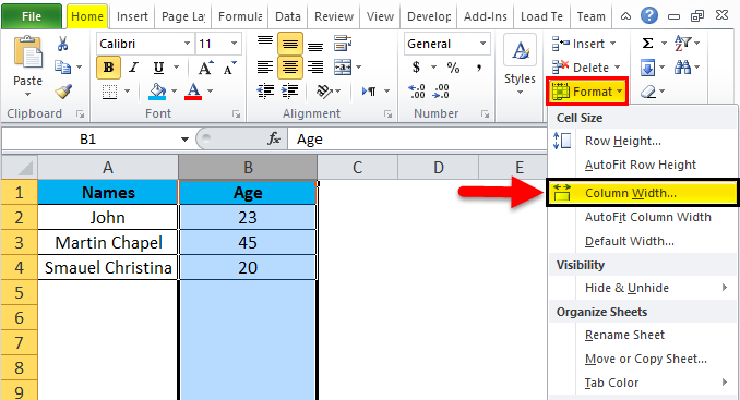
Excel row and column width size can be modified by using the format option in the HOME menu, which is shown below.
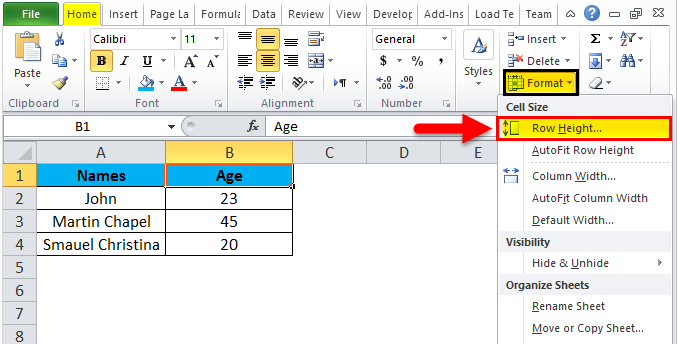
Using the format menu, we can change the row and column width where we have the list option, which are as follows:
- ROW HEIGHT– This is used to adjust the row height.
- AUTOFIT ROW HEIGHT– This will automatically adjust the row height.
- COLUMN WIDTH – This is used to adjust column width.
- AUTOFIT COLUMN WIDTH– This will automatically adjust the column width.
Let’s consider the below example to change the row and column width. Follow the below steps.
Step 1 – First, select the second row as shown in the below screenshot.
Step 2 – Go to the Format menu and click on ROW HEIGHT, as shown below.
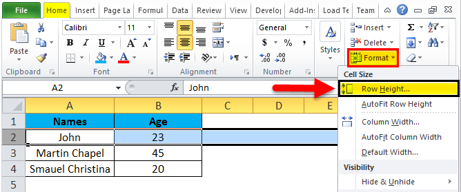
Step 3 – Once we select the ROW HEIGHT, we will get the below dialog box to change the height of the row.
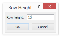
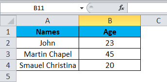
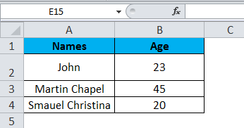
Step 4 – Now increase the row height to 25 so that the selected row height will get increased, as shown in the below screenshot.

We can see that row height has been increased when compared to the previous one; alternatively, we can change the row height by using the mouse.
Step 5 – Now go to the second option in the format list called AUTOFIT ROW HEIGHT, which will automatically reset the row to its original height.
Step 6 – Select the same row and go to the Format menu.
Step 7 – Now select the “AutoFit Row Height” as shown below.
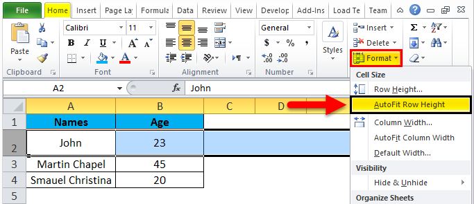
Once we click on the “AutoFit Row Height” option, the row height will reset to the original position, shown below.
Adjusting Column Width
We can adjust the column width in the same way by using the format option.
Step 1 – First, click on the cell B cell as shown below.
Step 2 – Now go to the Format menu and click on column width as shown in the below screenshot.
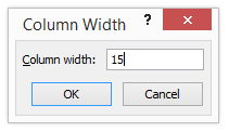
Once we click on the Column width, we will get the below dialog box to increase the column width, as shown below.
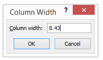
Step 3 – Now increase the column width by 15 to increase the selected column width.
In the above screenshot, we can see that column width has been increased; alternatively, we can adjust the column width by using the mouse where if we place the mouse cursor, we will get the + plus mark sign near to the column.
Step 4 – Now click on the next option called “AutoFit Column width”. So that the selected column will get reset to its original size, which is shown below.
Things to Remember
- In excel, we can delete and insert multiple rows and columns.
- We can hide the specific row and columns using the hide option.
- Row and column cells can be protected by locking the specific cells.
Recommended Articles
This has been a guide to Rows and Columns in Excel. Here we also discuss Rows and Columns in Excel along with practical examples and downloadable excel template. You can also go through our other suggested articles –
- Excel Compare Two Columns
- Unhide Columns in Excel
- Sort Columns in Excel
- Excel Columns to Rows