
Home > Microsoft Excel > How to Use the Excel Collapse Rows Feature? — 4 Easy Steps
(Note: This guide on the Excel collapse rows feature is suitable for all Excel versions including Office 365.)
If you ever had to use an Excel sheet with thousands of rows, you will certainly agree that it was a daunting task. It is definitely confusing to keep track and analyze all the information, especially with complex spreadsheets.
Thankfully, Excel has an option to collapse certain rows temporarily and group them together for later use. These collapsed rows can be expanded later to the original view and used as usual. This feature will help you create compact and easy-to-read spreadsheets.
For example, let’s assume you have a large worksheet. You wish to view only certain rows that summarize the data in subtotals or grand total. To do this, you can use the Excel collapse rows feature.
In this guide, I’ll teach you how to collapse rows in Excel the easy way.
You’ll learn:
- How to Use the Excel Collapse Rows Feature?
- How to Use a Nested Collapse?
- How to Expand Collapsed Rows?
- How to Clear Collapsed Rows?
- How to Copy and Paste Visible Rows?
Related:
How to Delete a Pivot Table in Excel? 4 Best Methods
How to Indent in Excel? 3 Easy Methods
How to Use the Format Painter Excel Feature? — 3 Bonus Tips
How to Use the Excel Collapse Rows Feature?
Although it might look complicated at first, the Excel collapse rows feature is quite simple to use.
Just follow these steps:
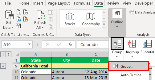
- Make sure that the excel worksheet is in a structured format with properly organized data.
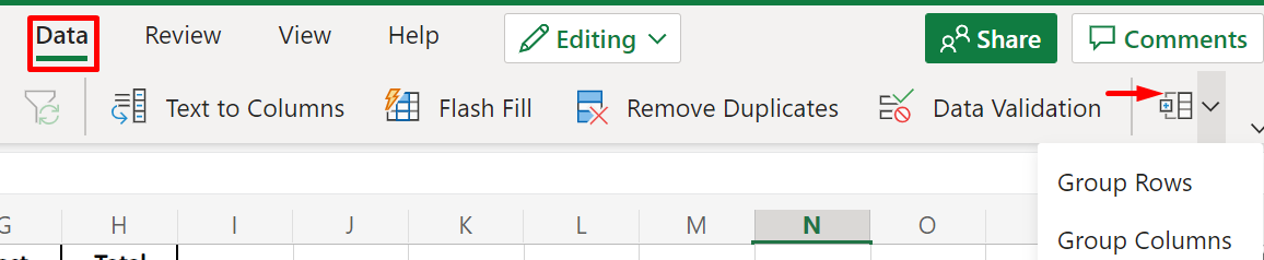
- Select the rows that you wish to collapse, then click on the Data tab and Groups in the Outline group, and then click on Group Rows.
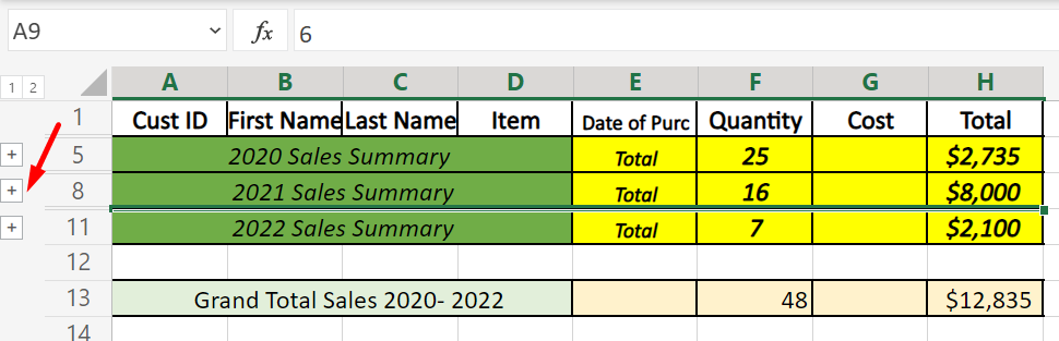
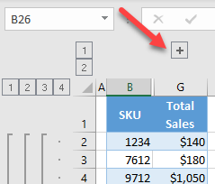
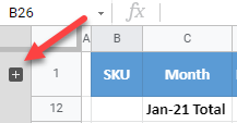
- You will see a ‘-’ sign on the left of column A. When you click on the ‘-’ sign, the selected rows get collapsed. Now the ‘-’ sign changes to ‘+’ which denotes that the rows are hidden.
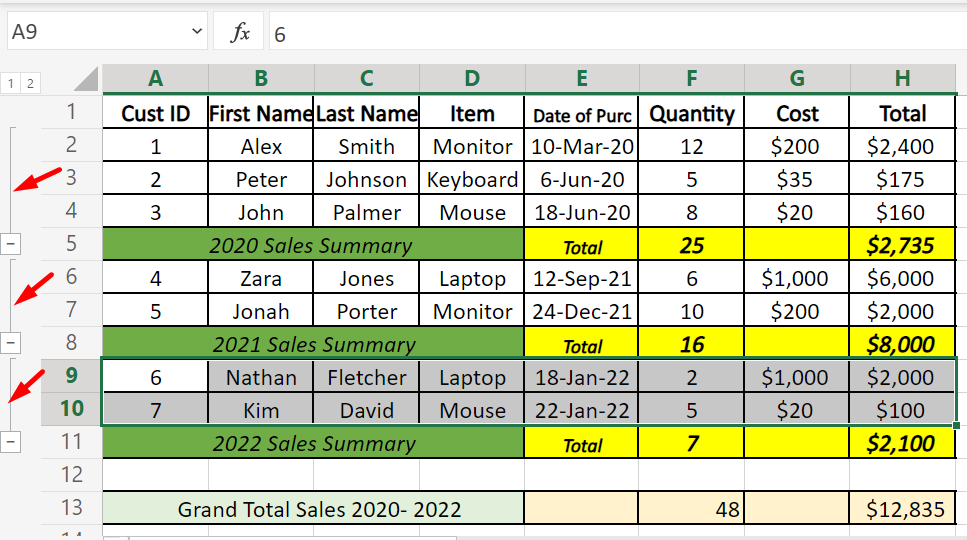
- Now, toggle between the + and – signs to collapse and expand the rows.
Also Read:
How to Use Goal Seek in Excel? (3 Simple Examples)
How to Insert Multiple Rows in Excel? The 4 Best Methods
How to Autofit Excel Cells? 3 Best Methods
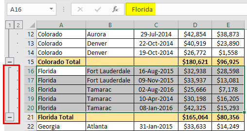
How to Use a Nested Collapse?
If you want to collapse rows inside already existing collapsed rows, repeat the same process. Select the rows and go to Data > Group Rows.
This will nest them together in groups, as shown below.
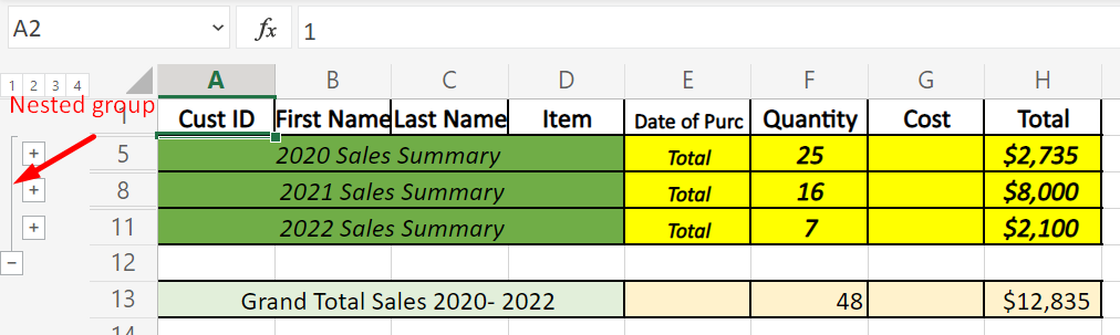
You can add more nested groups if required. If you feel that you no longer need the rows to be collapsed, just click on the Ungroup option in the Outline feature under the Data tab.
This will first ungroup the outer levels first.
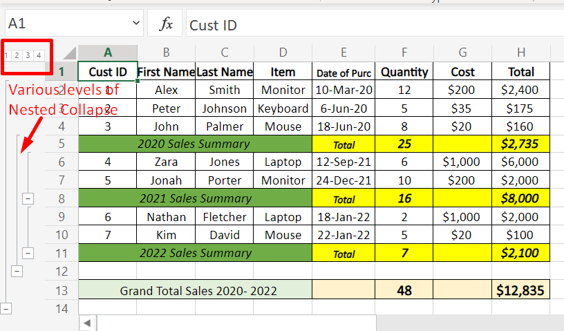
At the top left of the worksheet, you will find level buttons 1,2,3, and 4. These can also be used to expand and collapse the rows at each level of nesting.
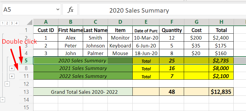
How to Expand Collapsed Rows?
You can click on the ‘+’ sign to show the hidden rows to expand the collapsed rows. Alternatively, you can also double click on the twin lines appearing in the collapsed rows area.
How to Clear Collapsed Rows?
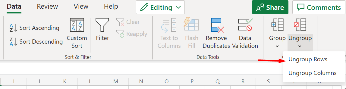
The hidden rows can be brought back by clicking on the Data -> Outline -> Ungroup – > Ungroup Rows. It starts by clearing the collapsed rows at the outer level and proceeds to clear the inner level.
You can also see the level buttons at the top-left corner of the worksheet disappearing.
How to Copy and Paste Visible Rows?
If you wish to copy only the visible rows follow these steps:
- First, select the visible rows you want to copy.
- Then, go to Home -> Editing -> Find & Select -> Go To Special and click on Visible Cells Only.


- Press Ctrl+C or right-click on the selected rows and select Copy.
- Paste the copied cells in a different location.
Suggested Reads:
How to Group Worksheets in Excel? (In 3 Simple Steps)
How to Shade Every Other Row in Excel? (5 Best Methods)
How to Use the Excel Fill Handle Easily? (Top 3 Uses with Examples)
Closing Thoughts
In this guide we saw how to collapse rows in Excel, make use of nested collapse, expand the rows and clear the collapsed rows.
The Excel collapse rows option is a very useful and lesser-known feature in Excel. Do use it to make your spreadsheets user-friendly.
You can find more high-quality Excel guides in our free resources center.
Simon Sez IT has been teaching critical IT software for over ten years. For a low, monthly fee you can get access to 100+ IT training courses by seasoned professionals.
Simon Calder

Chris “Simon” Calder was working as a Project Manager in IT for one of Los Angeles’ most prestigious cultural institutions, LACMA.He taught himself to use Microsoft Project from a giant textbook and hated every moment of it. Online learning was in its infancy then, but he spotted an opportunity and made an online MS Project course — the rest, as they say, is history!
Contents
- 1 How do I make rows collapsible and expandable in Excel?
- 2 What is the shortcut to expand all collapsed rows in Excel?
- 3 How do you expand rows quickly in Excel?
- 4 How do you Uncollapse rows in Excel?
- 5 How do I make Excel columns collapsible?
- 6 How do I widen multiple rows in Excel?
- 7 What is the shortcut key for Expand?
- 8 How do you expand grouping in Excel?
- 9 How do you expand all rows in Excel to show text?
- 10 How do you expand a row?
- 11 How do you collapse rows in sheets?
- 12 How do you multiply on Excel?
- 13 What are the shortcut key to group rows so you can expand?
- 14 How do you collapse all or code?
- 15 How do I collapse Visual Studio?
- 16 Can you expand all groups in Excel?
- 17 How do I expand an Excel spreadsheet?
- 18 Why can’t I expand a cell in Excel?
- 19 How do you keep a table expandable by inserting a table row?
- 20 How do I view all rows in Excel?
How do I make rows collapsible and expandable in Excel?
To add collapsible Excel rows, simply select the rows you want to collapse and use the Outline feature under the Data tab to group them. You can then click the plus and minus symbols on the left to collapse and expand, or the numbers at the top to collapse all and expand all.
What is the shortcut to expand all collapsed rows in Excel?
Press the “Ctrl-Shift-(” keys together to expand all hidden rows in your Excel spreadsheet.
How do you expand rows quickly in Excel?
Select the row or rows that you want to change. On the Home tab, in the Cells group, click Format. Under Cell Size, click AutoFit Row Height. Tip: To quickly autofit all rows on the worksheet, click the Select All button, and then double-click the boundary below one of the row headings.
How do you Uncollapse rows in Excel?
How to unhide all rows in Excel
- To unhide all hidden rows in Excel, navigate to the “Home” tab.
- Click “Format,” which is located towards the right hand side of the toolbar.
- Navigate to the “Visibility” section.
- Hover over “Hide & Unhide.”
- Select “Unhide Rows” from the list.
How do I make Excel columns collapsible?
About This Article
- Click the Data tab.
- Click Group.
- Select Columns and click OK.
- Click – to collapse.
- Click + to uncollapse.
How do I widen multiple rows in Excel?
Resize rows
- Select a row or a range of rows.
- On the Home tab, in the Cells group, select Format > Row Width.
- Type the row width and select OK.
What is the shortcut key for Expand?
Expand / Close All
Where you see braces or regions in code, you can collapse or expand them with the keyboard shortcut Ctrl + M, P to expand or Ctrl + M, O to collapse.
How do you expand grouping in Excel?
Add more grouping levels if necessary
To have it done, select all the rows except for the Grand Total row (rows 2 through 17), and click Data tab > Group button > Rows. As shown in the screenshot below, our data is now grouped in 4 levels: Level 1: Grand total. Level 2: Region totals.
How do you expand all rows in Excel to show text?
Adjust the row height to make all wrapped text visible
- Select the cell or range for which you want to adjust the row height.
- On the Home tab, in the Cells group, click Format.
- Under Cell Size, do one of the following: To automatically adjust the row height, click AutoFit Row Height.
How do you expand a row?
Click the button above the row 1 heading and to the left of the column A heading to select your entire sheet. Right-click on one of the row numbers, then left-click the Row Height option. Enter the desired height for your rows, then click the OK button.
How do you collapse rows in sheets?
To hide multiple rows in a Google Spreadsheet, click on the first row and drag across the rows you wish to hide, or hold the Shift key and click on the last row you want to hide. Then right click and select Hide rows X – X, where X indicates the numbers of the rows you have selected.
How do you multiply on Excel?
How to multiply two numbers in Excel
- In a cell, type “=”
- Click in the cell that contains the first number you want to multiply.
- Type “*”.
- Click the second cell you want to multiply.
- Press Enter.
- Set up a column of numbers you want to multiply, and then put the constant in another cell.
What are the shortcut key to group rows so you can expand?
#5 – Group or Ungroup Rows or Columns
Row and Column groupings are a great way to quickly hide and unhide columns and rows. Shift+Alt+Right Arrow is the shortcut to group rows or columns. Shift+Alt+Left Arrow is the shortcut to ungroup.
How do you collapse all or code?
Fold All:
- Windows: Ctrl + K Ctrl + 0.
- Mac: ⌘ + K ⌘ + 0.
How do I collapse Visual Studio?
CTRL + M + O will collapse all. CTRL + M + P will expand all and disable outlining. CTRL + M + M will collapse/expand the current section.
Can you expand all groups in Excel?
Grouping Rows or Columns
Groups and outlines allow you to quickly hide and unhide rows or columns in an Excel spreadsheet. The Groups feature creates row and column groupings in the Headings section of the worksheet. Each group can be expanded or collapsed with the click of a button.
How do I expand an Excel spreadsheet?
You can shrink or enlarge a worksheet for a better fit on printed pages. To do that, in Page Setup, click the window launcher button. Then, click Scaling > Adjust to, and then enter the percentage of the normal size that you want to use.
Why can’t I expand a cell in Excel?
If the height doesn’t expand to fit the contents of the cell, follow these steps, after doing the previous steps: Select the row. Make sure the Home tab of the ribbon is displayed.Choose AutoFit Row Height from the menu.
How do you keep a table expandable by inserting a table row?
Select the cells in the table you need to assign new data into except the formula column, then press the Ctrl + 1 keys to open the Format Cells dialog box. In the Format Cells dialog box, uncheck the Locked box, and then click the OK button.
How do I view all rows in Excel?
Once the entire sheet is selected, you can unhide all rows by doing one of the following:
- Press Ctrl + Shift + 9 (the fastest way).
- Select Unhide from the right-click menu (the easiest way that does not require remembering anything).
- On the Home tab, click Format > Unhide Rows (the traditional way).
In this tutorial, you will learn how to expand and collapse rows or columns by grouping them in Excel and Google Sheets.
Excel allows us to group and ungroup data, which enables us to expand or collapse rows and columns to better organize our spreadsheets. This is possible by grouping data manually or using the Auto Outline option.
Group and Ungroup Rows Manually
If we want to group rows in Excel, we need to have data organized in a way that’s compatible with Excel’s grouping functionality. This means that we need several levels of information sorted correctly and subtotals for each level of information that we want to group. Also, data must not have any blank rows or spaces.
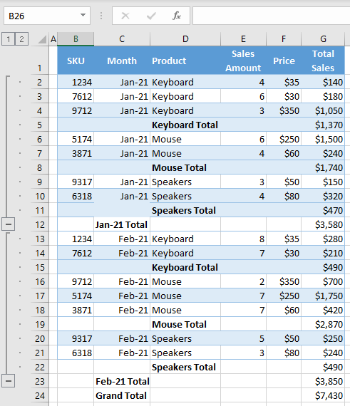
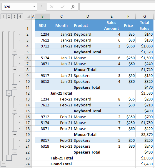
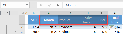
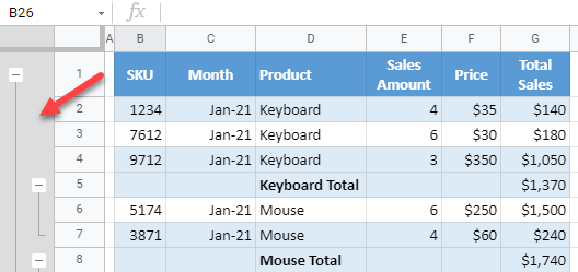
In the following example, we have total sales per month by product. Therefore, data are sorted by month and product and we have subtotals for each month, as we want to group data by month.
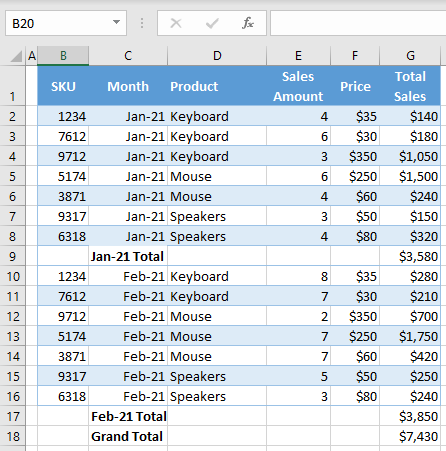
To group data for Jan-21 and Feb-21:
1. (1) Select data in the column that we want to group. In our case that is Jan-21, so we’ll select C2:C8. Then, in the Ribbon, (2) go to the Data tab, and in the Outline section, (3) click on the Group icon. (Note that you could also use a keyboard shortcut instead: ALT + SHIFT + right arrow).

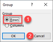
3. In the new window, leave Rows selected since we want to group rows and click OK.
As a result, we get the outline bar on the left side with Jan-21 grouped.
4. If we want to collapse this group of data, we just need to click on the minus sign in the outline bar.
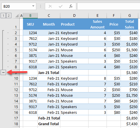
As shown in the picture below, all rows with Jan-21 in Column C are collapsed now and only the subtotal for this period remains visible.
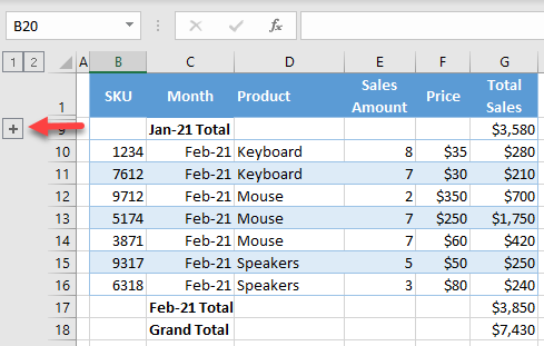
5. As in Step 4, we can expand the group (displaying rows) again, by clicking the plus sign. Following the exact same steps, we can also group data for Feb-21.
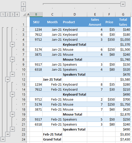
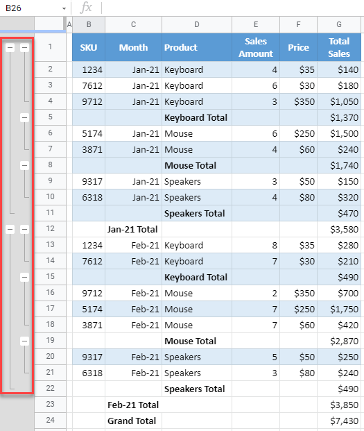
Group and Ungroup Multiple Levels of Data
Say we want to add another level of data grouping: Product. First, add a subtotal for all products.
Currently, we have two groups for Month level and subtotals for months and products. Now, we want to add groups for products. We can do this in the exact same way as we did for months. In this case, we’ll add six groups of data, selecting – separately – Keyboard (D2:D4), Mouse (D6:D7), etc. As a result, our data and outline bars look like the picture below.
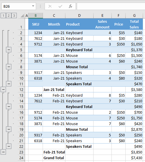
We now have two outline bars and the second one represents groups of products. Therefore, we can collapse all product groups, and have data organized in a way that displays only subtotals per month per product.
Group and Ungroup Rows Using Auto Outline
Instead of creating groups manually, we can also let Excel auto outline our data. This means that, if we have well-structured data, Excel will recognize groups and group data automatically.
To let Excel outline the data automatically, (1) click anywhere in the data, then in the Ribbon, (2) go to the Data tab, click on the arrow below the Group icon, and (3) choose Auto Outline.
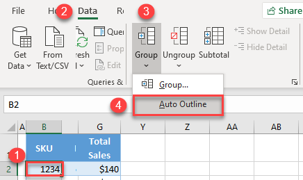
We get almost the same outline bars as in the manual example because Excel can recognize data groups. The only difference is that the Auto Outline option creates one group more for Grand Total, which can collapse all the data except the Total.
To remove outline bars created by Auto Outline, (1) click anywhere in the data then in the Ribbon, (2) go to the Data tab, click on the arrow below the Ungroup icon, and choose (3) Clear Outline.
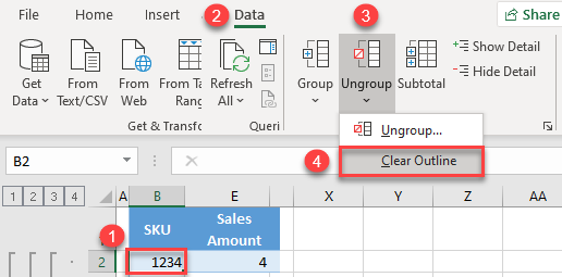
This will remove all outline bars and ungroup all data.
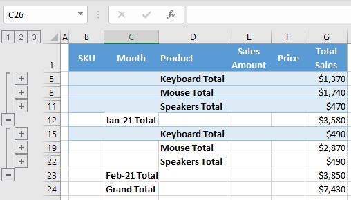
Expand and Collapse Entire Outline
Say we want to collapse the entire outline (for example, Month). In the outline bar, at the top, click on the outline bar number we want to collapse (in our case, outline level 2).
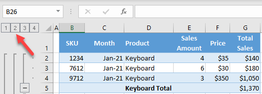
As a result, all rows with Jan-21 and Feb-21 are collapsed and only the totals are displayed.
If we want to expand the entire outline again, (1) click on Grand Total, then in the Ribbon, (2) go to the Data tab, and in the Outline section, (3) click on Show Detail.
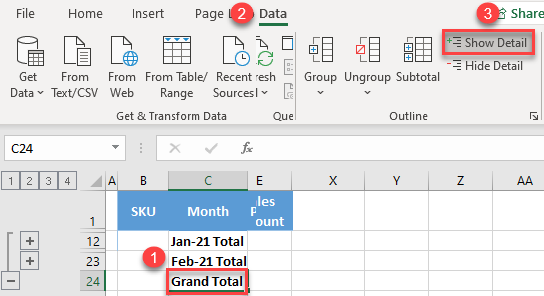
Now all data is visible again, and the Month outline is expanded.
Group and Ungroup Columns Manually
Similarly, we can also group columns in Excel. Say we want to display only SKU and the corresponding Total Sales.
1. Select all column headings that we want to group (in our case C1:F1).
2. In the Ribbon, go to the Data tab, and in the Outline section, choose Group (or use the keyboard shortcut ALT + SHIFT + right arrow).
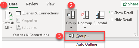
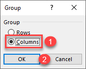
2. In the pop-up screen, (1) select Columns and (2) click OK.
As a result, we will get a new outline bar, but this time for the columns.
3. To collapse the group of columns, click on the minus sign at the end of the outline bar.
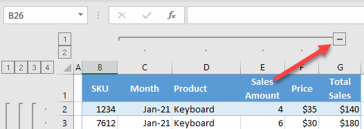
As a result, Columns C:F are collapsed.
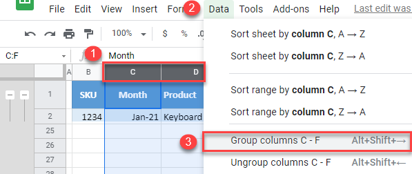
Group and Ungroup Rows in Google Sheets
In Google Sheets, we can only group rows manually, so let’s use the same example and see how to group data into the same categories. To group by month:
1. (1) Select all rows with Jan-21, then in the menu, (2) go to Data, and click on (3) Group.
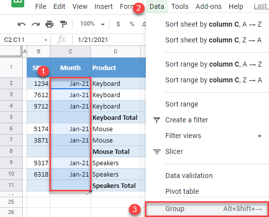
2. In the new window beside the selection, click on Group rows 2 – 11.
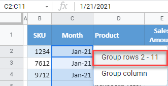
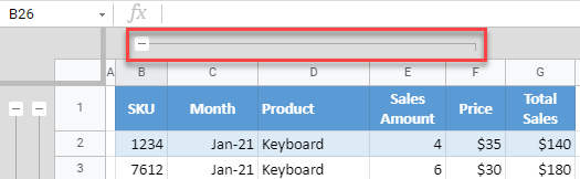
Jan-21 (Rows 2–11) are now grouped, and we can see the outline bar on the left side. The difference compared to Excel, is that the minus/plus sign for collapse/expand is a the top of each group.
3. To collapse Jan-21, click the minus sign at the top of the outline bar for months.
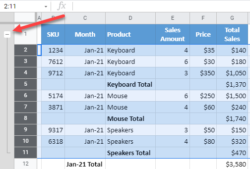
Now, data for the month are collapsed, and we can see only the Jan-21 Total row.
4. We now get the plus sign, so we can expand the group again.
5. Following these steps, we can also group Feb-21 and create a new outline for the Product data level. When we’re done, the data and outline bars should look like this:
Ungrouping data in Google Sheets works just like grouping.
1. (1) Select the data we want to ungroup (Keyboard in Jan-21– cells D2:D4), then in the menu, (2) go to Data, and (3) click on Ungroup.
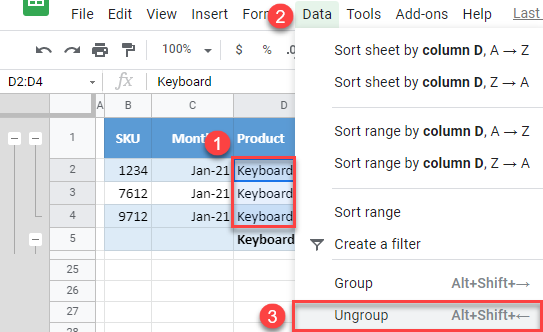
2. In the new window beside the selection, click on Ungroup rows 2 – 4.
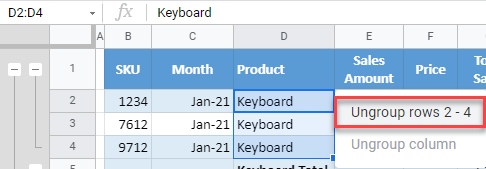
Those three rows are now ungrouped and removed from the outline bar.
Group and Ungroup Columns in Google Sheets
Grouping columns can be done in a similar way to grouping rows.
Select Columns C:F, then in the menu, go to Data, and click on Group columns C – F.
Now, we get the outline bar for column grouping.
To ungroup columns, select Columns C:F, go to Data, and click on Ungroup columns C – F.
Working on a sheet containing thousands of rows will definitely make you tired. Nobody would like to keep track of all the data and it becomes more daunting with a complex sheet. Excel lets you collapse rows easily by using multiple features and you can group them for later use. You can expand these Excel collapse rows quickly and convert them to their original form.
Let’s follow the below-given methods to understand how you can collapse rows in Excel.
Excel Collapse Rows Feature
Excel for some users is nothing more than a sheet containing unlimited cells that made rows and columns. When the dataset is large enough to handle, you can take Excel’s help and put that data into these rows and columns for a better understanding. The grouping feature in Excel lets you collapse rows easily.
For Excel collapse rows with headers, you will definitely be needing to add some thought into how you can do this when the sheet is all set up.
How Excel Collapse Rows with Context Menu?
Hiding rows in Excel by using the context menu is one of the main approaches you can use. In our dataset, you can see three orders for bananas. Let’s see how you can hide them:
- First, choose the rows that have orders for Banana, such as rows 5, 6, and 7.

- Right-click on the mouse and then click on the “Hide” button from the Context Menu.

- You will notice that rows 5, 6, and 7 are collapsed.

Excel Collapse Rows with Filtering
Filtering rows to hide them from a large collection of data is possible with data analysis in Excel. Let’s see how it happens:
- First, select the entire dataset.

- From the Excel, Ribbon choose the Data Tab and then Filter.

- Click on the down arrows that appear there. It will give you the option to filter rows based on specific criteria.

- In the Category column, choose the down arrow. Check the Fruit option given in the context menu and press OK.

You will notice the dataset is now filtered for Fruit items only and Vegetable rows have been collapsed.

Excel Collapse Rows with Keyboard Shortcuts
Using a keyboard shortcut is the first approach for many Excel users. Excel every time provides shortcuts to save time and effort. This time for hiding rows, Excel gives us effectively used keyboard shortcuts. Let’s dive in to see how it happens:
- First, choose the rows such as 5 – 10.

- Now press the shortcut command:
ALT + H + O + R

Things to Consider
While using keyboard shortcuts, follow the given keys as well:
- To select the entire column in the dataset:
Press SHIFT + Space
- To group selected rows:
Press SHIFT + ALT + Right Arrow key
- To ungroup rows:
Press SHIFT + ALT + Left Arrow key
Wrap it Up
Now, you have learned the best methods for Excel collapse rows and columns. All you need to do is practice so that you can easily manage to perform any task quickly.
Filters or hiding cells serve the purpose when the underlying information belongs to the same category. But for those which have subsets, as in small groups within each larger group, these features provided by MS Excel does not deem to be fit. What else does Excel’s bags of tricks have got to offer on this occasion?
Also read: How to Hide Cells in MS Excel?
We are going to have a look at just that in the following sections & we would be using the following tabulation to demonstrate through each of the below methods,
- Selecting from Data Tab
- Keyboard Shortcut

Grouping of Rows:
To group any given data, one has to look into the commonalities that exist, which in the above dataset is the time period for 2021, which has been summarised under each Region. The given tabulation consists of four different regions with the sales details for a period of 12 months listed under each region.

There also exists a summary which contains the total of the sales numbers for that year at the very beginning.

That’s all for the briefing & your mission, should you choose to accept it is to group all 12 months under each region such that it would be easier to compare any two regions against each other in a single click.
Method 1 – Selecting from Data Tab:
Let us get started by selecting the rows of the 12 months given under the North region as shown in the below image.

Navigate your way using the cursor to the Data tab & that is where you will be finding the Group option.

What are you waiting for? Click on that option!
The following changes would be visible on your screen in a jiffy.

“Yeah, yeah! Enough of gimmicks & can you tell me what to do with those buttons in the above image?”
I’ve foreseen these voices of yours & here is what one can do. Click on the minus (-) button to collapse all the 12 months under the North region. Once done, the minus (-) button transforms itself into a plus (+) button & the 12 months has gone with the wind.

Repeat the same procedure for the other regions too such that all the rows with the months from Jan to Dec get hidden only to be summoned by the click of the plus (+) button.

Method 2 – Keyboard Shortcut:
The part where we select the rows of the months under a region remains the same as stated in the previous method. The difference kicks in now.
Rather than moving the cursor, one shall place the fingers over the keys of the keyboard. Which keys do you ask?
These!
SHIFT + ALT + RIGHT ARROW KEY (→)
Much emphasis is on pressing the keys one after the other, similar to the way CTRL+C or CTRL+V is exercised. Trying to pull off anything else, would only render the execution of this shortcut unfeasible.
After the above keys are pressed in the same sequence, the selected rows would be collapsed as shown below.

The same technique is repeated to group & collapse the months of the other regions too.

Conclusion:
Hope the article was informative. Here is an additional lead to an article that might interest you! To know how to freeze columns in MS Excel, do have a look at this article. QuickExcel has numerous other articles too which could help you with that one thing that you’re trying to do with MS Excel right now. Cheers!
Grouping Rows in Excel
In Excel, organizing the large data by combining the subcategory data is called “grouping of rows.” When the number of items in line is not important, we can choose group rows that are not important but only see the subtotal of those rows. On the other hand, when the data rows are huge, scrolling down and reading the report may lead to a wrong understanding, so the grouping of rows helps us hide the unwanted numbers of rows.
The number of rows is also lengthy when the worksheet contains detailed information or data. However, report readers of the data do not want to see long rows. Instead, they want to see a clear view, but at the same time, if they require any other detailed information, they need just a button to expand or collapse them as needed.
This article will show you how to group rows in Excel with expand/collapse to maximize the report viewing technique.
Table of contents
- Grouping Rows in Excel
- How to Group Rows in Excel with Expand/Collapse?
- Group by Using Shortcut Key
- Example #1 – Using Auto Outline
- Example #2 – Using Subtotals
- Things to Remember here
- Recommended Articles
- How to Group Rows in Excel with Expand/Collapse?
How to Group Rows in Excel with Expand/Collapse?
You can download this Group Rows Excel Template here – Group Rows Excel Template
For example, look at the below data.
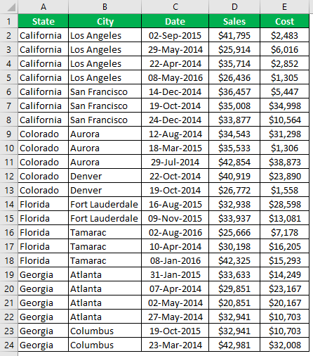
We have city and state-related sales and cost data in the table above. Still, when we look at the first two rows of the data, we have “California” state and the city is “Los Angeles,” but sales happened on different dates. Hence, as a report reader, everyone prefers to read the state-wise sales and city-wise sales in a single column, so we can create a single line summary view by grouping the rows.
Follow the below steps to group rows in excel.
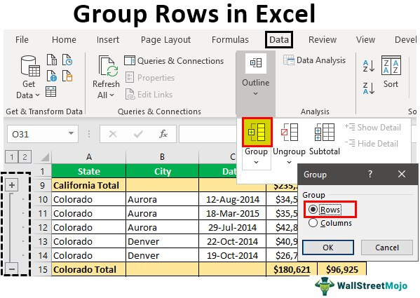
- First, we must create a subtotal like the one below.

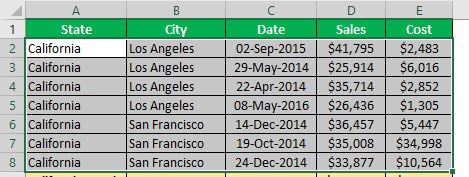
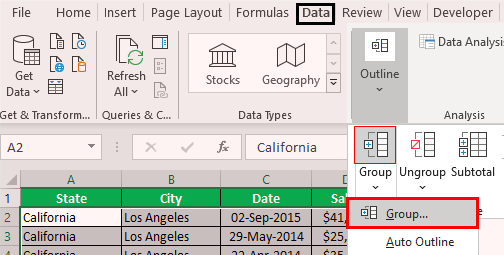
- We must select the first state rows (California state), excluding subtotals.

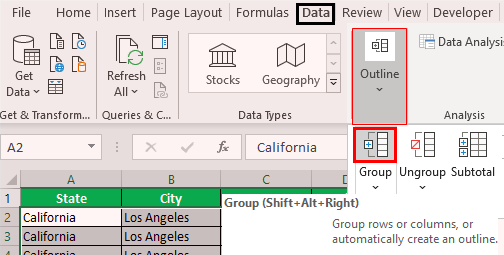
- Then, go to the Data tab and choose the “Group” option.

- Click on the drop-down list in excel of “Group” and choose “Group” again.
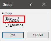
- Now, it may ask whether to group rows or columns. Since we are grouping Rows, we must choose Rows and click on OK.

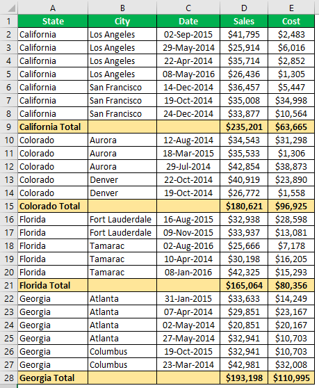
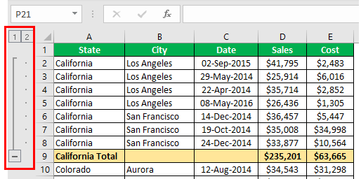
- The moment we click on OK, we can see a joint line on the left-hand side.

- Then, we must click on the minus icon and see the magic.

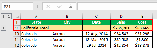
Now, we can see the total summary for the city California. Again, if we want to see a detailed overview of the city, we can click on the plus icon to expand the view. - Now again, select the city Colorado and click on the Group option.

- As a result, it will group for the Colorado state.


Group by Using Shortcut Key
With a simple shortcut in excelAn Excel shortcut is a technique of performing a manual task in a quicker way.read more, we can easily group selected rows or columns. The shortcut key to group the data is “SHIFT + ALT + Right Arrow key.”
![]()
First, we must select the rows that need to be grouped.

To group these rows, we must press the shortcut key “SHIFT + ALT + Right Arrow key.“
In the above, we have seen how to group the data and row with expanding and collapse options using the “PLUS” and “MINUS” icons.
The only problem with the above method is that we need to do this for each state individually, so this takes a lot of time when there are many states. So, what would be your reaction if we say you can group with just one click?
Amazing. Using the “Auto Outline,” we can automatically group the data.
Example #1 – Using Auto Outline
First we need to create subtotal rows.

Now, we must place a cursor inside the data range. Under the “Group” drop-down, we can see one more option other than “Group,” which is “Auto Outline.”

The moment we click on this “Auto Outline” option, it will group all the rows above the subtotal row.

How cool is this??? Very cool, isn’t it??
Example #2 – Using Subtotals
If grouping the rows for the individual city is the one problem, then even before grouping rows, there is another problem: adding subtotal rows.
When there are hundreds of states, it is a tough task to create a subtotal row for each state separately, so we can use the “Subtotal” option to create a subtotal for the selected column quickly.
For example, we had the data like the below before creating the subtotal.

Under the “Data” tab, we have an option called “Subtotal” right next to the “Group” option.

Click on this option by selecting any of the cells of the data range. It will show the below option first up.

First, select the column that needs a subtotal. In this example, we need subtotal for “State,” so choose the same from the drop-down list of “At each change in.”

Next, we need to select the function type since we add all the values to choose “Sum” function in excel.

Now, select the columns that need to be summed. We need the summary of the “Sales“and “Cost” columns, so choose the same. Click on “OK.”

We will have subtotal rows shortly.

Did you notice one special thing from the above image???
It has automatically grouped rows for us!!!!
Things to Remember here
- The shortcut key for grouping rows is the “Shift + ALT + Right Arrow” key.
- We should sort subtotal that needs data.
- The “Auto Outline” option can group all the rows above the subtotal row.
Recommended Articles
This article is a guide to Group Rows in Excel. We discuss grouping rows in Excel with expand/collapse using an auto outline and subtotal options with examples and a downloadable Excel template. You may also look at these useful functions in Excel: –
- Excel Maximum Number of Rows
- Divide Cell in ExcelDivide in Excel is used for division applications, where (/) is the symbol and we can write an expression =a/b, where a and b represent two numbers or values to be divided.read more
- Group Columns in ExcelIn Excel, grouping one or more columns together in a worksheet is referred to as group column and I t allows you to contract or expand the column.read more
- Group Worksheets In ExcelGrouping gives the best results to users when the same type of data is presented in the cells of the same addresses. Grouping also improves the accuracy of data and eliminates the error made by a human in performing the calculations.read more
Worksheet often comes up with a lot of detailed information that might be difficult to read and analyze. Fortunately, Microsoft Excel offers smart features to organize data in groups which allows the rows to be collapsible and expandable. In the compact view, one can easily analyze the whole content available in the Excel sheet.
Therefore, in this guidance, you will read about how to group rows in Excel and the best way to expand and collapse rows in Excel.
Grouping the rows in an Excel sheet is best for a structured worksheet that has a column heading and no blank rows, summary row for each subset of rows. With well- organized data, you can use the following ways to group rows in Excel.
Method 1: Create an Outline to Group Rows Automatically
If your data contains only one level of information then you can quickly let Excel group rows automatically for you. Below are the following steps on how to get it done.
Step 1: To begin, select one cell in any of the rows that you want to group.
Step 2: Next to this, you can go to the Data tab and click on the Outline group.

Step 3: Then, click the arrow under the Group option and select Auto Outline option.
Once you are done performing the above-mentioned steps, the rows will be grouped smoothly and the outline bars representing the different levels of the data have been added to the left before column A.
Note: if summary rows are located above a group of detail rows then before creating an outline, follow the following steps:
Step 1: Go to the Data tab and click the Outline group.
Step 2: Next to this, click the Outline dialog box and clear the Summary rows below detail option.
Step 3: Click on the OK button to successfully apply your actions.
When the outline is created, you can easily hide or show details within a certain group just by clicking the Minus (-) or Plus (+) sign for that group. Moreover, you can expand and collapse rows in Excel 2013. All you are required to click on the level buttons located at the top left corner of the Excel sheet.
Method 2: Group Rows Manually
If your Excel sheet contains two or more than two levels of information then Excel’s Auto Outline may not group the data correctly. In this scenario, you can simply group rows manually so that it does not affect your data and organizes it in a good manner. To do so, you can follow the steps mentioned below.
Note: Before you apply any actions to group rows, make sure there are no hidden rows in your data set otherwise your sheet might not be grouped properly.
Step 1: Create Outer Groups (Level 1)
- Choose one of the larger subsets of data. This should also include all of the intermediate summary rows and their detail rows.
- Now, on the Data tab, you can click on the Group button clicking (in the Outline group).
- After this, you can select Rows and click on the OK button.

This will quickly add a bar on the left of the Worksheet that stretches the selected rows. In this way, you can create as many as outer groups are needed.
Tip: To create new groups fastly, you can also use shortcuts. Press the Shift + Alt + Right Arrow keys together from your Keyboard.
Step 2: Create Nested Groups (Level 2)
- To create nested groups or inner groups, you can select all detail rows above the related summary row.
- Then, you can click the Group button.
- This will successfully create inner groups in your Excel sheet.
Step 3: Add More Grouping levels if Needed
In case more data is added to your Worksheet then you may require more grouping levels for which you need to create more outline levels. To do so, you can follow the steps mentioned below.
- Insert the Grand total row in the table.
- Then, add the outermost outline level.
- To make it happen, you can select all the rows except the Grand total row and click on the Data tab then Group button to select Rows.
How to Create Collapsible Rows in Excel?
In Excel, one of the most useful features of grouping is the ability to show and hide the detail rows for a particular group. In addition, you can collapse and expand the outline to a certain level in a few clicks. In this guide, you can learn how to expand and collapse rows in excel. To know the process of excel collapse rows, look for the following guidance.
Create Rows within a Group
If you want to learn how to collapse rows in excel 2013, you can use the Minus (-) sign located at the below of the group bar.
Another way to collapse rows in Excel sheets is to select any cell in the group. Then, you can click the Hide Detail button on the Data tab, in the Outline group.
This way, the group would be minimized to the summary row and the detail rows would be hidden.
How to Expand Rows in Excel?
To expand rows within a group, you can click any cell in the visible summary rows. Then, you can click the Show Detail button available on the Data tab, in the Outline group. Or, you can also use the Plus (+) sign in order to expand the collapsed group of rows.
How to Ungroup a Certain Group of Rows?
After grouping the rows, if you wish to ungroup them in the future then you can follow the following simple steps.
Step 1: First of all, select the rows that you want to ungroup.
Step 2: Go to the Data tab and click the Outline group.
Step 3: At this point, you can click on the Ungroup button or use Shift + Alt + Left Arrow shortcuts from your Keyboard.
Step 4: Now in the Ungroup dialog box, you can select the Rows option and hit the OK button.
Note: It is not easy to ungroup non-adjacent groups of rows. So, you will have to repeat the aforementioned steps for each group individually.
Conclusion
If you were seeking the easiest process for excel collapse rows, group rows in Excel or expand and collapse rows in excel then this particular guide is surely going to teach you how to group rows in excel with expand collapse in the simplest way.