
Excel for Microsoft 365 Excel for the web Excel 2021 Excel 2019 Excel 2016 Excel 2013 Excel 2010 More…Less
When you create a simple formula or a formula by that uses a function, you can refer to data in worksheet cells by including cell references in the formula arguments. For example, when you enter or select the cell reference A2, the formula uses the value of that cell to calculate the result. You can also reference a range of cells.
For more information about cell references, see Create or change a cell reference. For more information about formulas in general, see Overview of formulas.
-
Click the cell in which you want to enter the formula.
-
In the formula bar
 , type = (equal sign).
 -
Do one of the following, select the cell that contains the value you want or type its cell reference.
You can refer to a single cell, a range of cells, a location in another worksheet, or a location in another workbook.
When selecting a range of cells, you can drag the border of the cell selection to move the selection, or drag the corner of the border to expand the selection.
1. The first cell reference is B3, the color is blue, and the cell range has a blue border with square corners.
2. The second cell reference is C3, the color is green, and the cell range has a green border with square corners.
Note: If there is no square corner on a color-coded border, the reference is to a named range.
-
Press Enter.
 , type = (equal sign).
Example
Copy the example data in the following table, and paste it in cell A1 of a new Excel worksheet. For formulas to show results, select them, press F2, and then press Enter. If you need to, you can adjust the column widths to see all the data. Use the Define Name command (Formulas tab, Defined Names group) to define «Assets» (B2:B4) and «Liabilities» (C2:C4).
|
Department |
Assets |
Liabilities |
|
IT |
274000 |
71000 |
|
Admin |
67000 |
18000 |
|
HR |
44000 |
3000 |
|
Formula |
Description |
Result |
|
‘=SUM(Assets) |
Returns the total of the assets for the three departments in defined name «Assets,» which is defined as the cell range B2:B4. (385000) |
=SUM(Assets) |
|
‘=SUM(Assets)-SUM(Liabilities) |
Subtracts the sum of the defined name «Liabilities» from the sum of the defined name «Assets.» (293000) |
=SUM(Assets)-SUM(Liabilities) |
Top of Page
Need more help?
Want more options?
Explore subscription benefits, browse training courses, learn how to secure your device, and more.
Communities help you ask and answer questions, give feedback, and hear from experts with rich knowledge.
Excel for Microsoft 365 Excel for the web Excel 2021 Excel 2019 Excel 2016 Excel 2013 Excel 2010 Excel 2007 More…Less
A cell reference refers to a cell or a range of cells on a worksheet and can be used in a formula so that Microsoft Office Excel can find the values or data that you want that formula to calculate.
In one or several formulas, you can use a cell reference to refer to:
-
Data from one or more contiguous cells on the worksheet.
-
Data contained in different areas of a worksheet.
-
Data on other worksheets in the same workbook.
For example:
|
This formula: |
Refers to: |
And Returns: |
|---|---|---|
|
=C2 |
Cell C2 |
The value in cell C2. |
|
=A1:F4 |
Cells A1 through F4 |
The values in all cells, but you must press Ctrl+Shift+Enter after you type in your formula. Note: This functionality doesn’t work in Excel for the web. |
|
=Asset-Liability |
The cells named Asset and Liability |
The value in the cell named Liability subtracted from the value in the cell named Asset. |
|
{=Week1+Week2} |
The cell ranges named Week1 and Week2 |
The sum of the values of the cell ranges named Week1 and Week 2 as an array formula. |
|
=Sheet2!B2 |
Cell B2 on Sheet2 |
The value in cell B2 on Sheet2. |
-
Click the cell in which you want to enter the formula.
-
In the formula bar
, type = (equal sign). -
Do one of the following:
-
Reference one or more cells To create a reference, select a cell or range of cells on the same worksheet.
You can drag the border of the cell selection to move the selection, or drag the corner of the border to expand the selection.
-
Reference a defined name To create a reference to a defined name, do one of the following:
-
Type the name.
-
Press F3, select the name in the Paste name box, and then click OK.
Note: If there is no square corner on a color-coded border, the reference is to a named range.
-
-
-
Do one of the following:
-
If you are creating a reference in a single cell, press Enter.
-
If you are creating a reference in an array formula (such A1:G4), press Ctrl+Shift+Enter.
The reference can be a single cell or a range of cells, and the array formula can be one that calculates single or multiple results.
Note: If you have a current version of Microsoft 365, then you can simply enter the formula in the top-left-cell of the output range, then press ENTER to confirm the formula as a dynamic array formula. Otherwise, the formula must be entered as a legacy array formula by first selecting the output range, entering the formula in the top-left-cell of the output range, and then pressing CTRL+SHIFT+ENTER to confirm it. Excel inserts curly brackets at the beginning and end of the formula for you. For more information on array formulas, see Guidelines and examples of array formulas.
-
You can refer to cells that are on other worksheets in the same workbook by prepending the name of the worksheet followed by an exclamation point (!) to the start of the cell reference. In the following example, the worksheet function named AVERAGE calculates the average value for the range B1:B10 on the worksheet named Marketing in the same workbook.

1. Refers to the worksheet named Marketing
2. Refers to the range of cells between B1 and B10, inclusively
3. Separates the worksheet reference from the cell range reference
-
Click the cell in which you want to enter the formula.
-
In the formula bar
, type = (equal sign) and the formula you want to use. -
Click the tab for the worksheet to be referenced.
-
Select the cell or range of cells to be referenced.
Note: If the name of the other worksheet contains nonalphabetical characters, you must enclose the name (or the path) within single quotation marks (‘).
Alternatively, you can copy and paste a cell reference and then use the Link Cells command to create a cell reference. You can use this command to:
-
Easily display important information in a more prominent position. Let’s say that you have a workbook that contains many worksheets, and on each worksheet is a cell that displays summary information about the other cells on that worksheet. To make these summary cells more prominent, you can create a cell reference to them on the first worksheet of the workbook, which enables you to see summary information about the whole workbook on the first worksheet.
-
Make it easier to create cell references between worksheets and workbooks. The Link Cells command automatically pastes the correct syntax for you.
-
Click the cell that contains the data you want to link to.
-
Press Ctrl+C, or go to the Home tab, and in the Clipboard group, click Copy
.
-
Press Ctrl+V, or go to the Home tab, in the Clipboard group, click Paste
.By default, the Paste Options
button appears when you paste copied data. -
Click the Paste Options button, and then click Paste Link
.
 .
.
 .
. button appears when you paste copied data.
 .
.-
Double-click the cell that contains the formula that you want to change. Excel highlights each cell or range of cells referenced by the formula with a different color.
-
Do one of the following:
-
To move a cell or range reference to a different cell or range, drag the color-coded border of the cell or range to the new cell or range.
-
To include more or fewer cells in a reference, drag a corner of the border.
-
In the formula bar
, select the reference in the formula, and then type a new reference. -
Press F3, select the name in the Paste name box, and then click OK.
-
-
Press Enter, or, for an array formula, press Ctrl+Shift+Enter.
Note: If you have a current version of Microsoft 365, then you can simply enter the formula in the top-left-cell of the output range, then press ENTER to confirm the formula as a dynamic array formula. Otherwise, the formula must be entered as a legacy array formula by first selecting the output range, entering the formula in the top-left-cell of the output range, and then pressing CTRL+SHIFT+ENTER to confirm it. Excel inserts curly brackets at the beginning and end of the formula for you. For more information on array formulas, see Guidelines and examples of array formulas.
Frequently, if you define a name to a cell reference after you enter a cell reference in a formula, you may want to update the existing cell references to the defined names.
-
Do one of the following:
-
Select the range of cells that contains formulas in which you want to replace cell references with defined names.
-
Select a single, empty cell to change the references to names in all formulas on the worksheet.
-
-
On the Formulas tab, in the Defined Names group, click the arrow next to Define Name, and then click Apply Names.
-
In the Apply names box, click one or more names, and then click OK.
-
Select the cell that contains the formula.
-
In the formula bar
, select the reference that you want to change. -
Press F4 to switch between the reference types.
For more information about the different type of cell references, see Overview of formulas.
-
Click the cell in which you want to enter the formula.
-
In the formula bar
, type = (equal sign). -
Select a cell or range of cells on the same worksheet. You can drag the border of the cell selection to move the selection, or drag the corner of the border to expand the selection.
-
Do one of the following:
-
If you are creating a reference in a single cell, press Enter.
-
If you are creating a reference in an array formula (such A1:G4), press Ctrl+Shift+Enter.
The reference can be a single cell or a range of cells, and the array formula can be one that calculates single or multiple results.
Note: If you have a current version of Microsoft 365, then you can simply enter the formula in the top-left-cell of the output range, then press ENTER to confirm the formula as a dynamic array formula. Otherwise, the formula must be entered as a legacy array formula by first selecting the output range, entering the formula in the top-left-cell of the output range, and then pressing CTRL+SHIFT+ENTER to confirm it. Excel inserts curly brackets at the beginning and end of the formula for you. For more information on array formulas, see Guidelines and examples of array formulas.
-
You can refer to cells that are on other worksheets in the same workbook by prepending the name of the worksheet followed by an exclamation point (!) to the start of the cell reference. In the following example, the worksheet function named AVERAGE calculates the average value for the range B1:B10 on the worksheet named Marketing in the same workbook.
1. Refers to the worksheet named Marketing
2. Refers to the range of cells between B1 and B10, inclusively
3. Separates the worksheet reference from the cell range reference
-
Click the cell in which you want to enter the formula.
-
In the formula bar
, type = (equal sign) and the formula you want to use. -
Click the tab for the worksheet to be referenced.
-
Select the cell or range of cells to be referenced.
Note: If the name of the other worksheet contains nonalphabetical characters, you must enclose the name (or the path) within single quotation marks (‘).
-
Double-click the cell that contains the formula that you want to change. Excel highlights each cell or range of cells referenced by the formula with a different color.
-
Do one of the following:
-
To move a cell or range reference to a different cell or range, drag the color-coded border of the cell or range to the new cell or range.
-
To include more or fewer cells in a reference, drag a corner of the border.
-
In the formula bar
, select the reference in the formula, and then type a new reference.
-
-
Press Enter, or, for an array formula, press Ctrl+Shift+Enter.
Note: If you have a current version of Microsoft 365, then you can simply enter the formula in the top-left-cell of the output range, then press ENTER to confirm the formula as a dynamic array formula. Otherwise, the formula must be entered as a legacy array formula by first selecting the output range, entering the formula in the top-left-cell of the output range, and then pressing CTRL+SHIFT+ENTER to confirm it. Excel inserts curly brackets at the beginning and end of the formula for you. For more information on array formulas, see Guidelines and examples of array formulas.
-
Select the cell that contains the formula.
-
In the formula bar
, select the reference that you want to change. -
Press F4 to switch between the reference types.
For more information about the different type of cell references, see Overview of formulas.
Need more help?
You can always ask an expert in the Excel Tech Community or get support in the Answers community.
Need more help?
Want more options?
Explore subscription benefits, browse training courses, learn how to secure your device, and more.
Communities help you ask and answer questions, give feedback, and hear from experts with rich knowledge.
Microsoft Excel, sometimes known as MS Excel, is a potent spreadsheet programme. In Excel, each worksheet consists of a number of cells that are made up of rows and columns. Each cell has a unique reference, which enables users to quickly access and address the required cell (or cells) within the functions. In Excel, cell references are crucial, particularly when working with huge data sets in functions and formulas.
This article covers a quick overview of Excel Cell References. The various sorts of cell references that Excel offers and the detailed instructions for using each one are also covered in the article.
What is a Cell Reference?
An Excel cell reference, also known as a cell address, is a mechanism that defines a cell on a worksheet by combining a column letter and a row number. We can refer to any cell (in Excel formulas) in the worksheet by using the cell references.
For example:
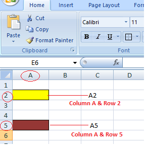
Here we refer to the cell in column A & row 2 by A2 & cell in column A & row 5 by A5. You can make use of such notations in any of the formulas or copy the value of one cell to another cell (by using = A2 or = A5).
Types of Cell Reference in Excel
Understanding various cell references primarily makes it easier for us to use Excel formulas and avoid unexpected formula errors. When copying and pasting Excel formulas, this is quite useful. Based on various use situations, Excel offers three main types of cell references, including:
- Relative Cell Reference
- Absolute Cell Reference
- Mixed Cell Reference
1. Relative Cell Reference
In Excel, a relative cell reference is used by default. Excel uses a relative reference whenever we insert a cell reference or a range within a formula. The relative references, which commonly reflect the combination of column name and row number, are used normally with the associated cell references. There is no dollar ($) sign in the relative reference for the cell.
How to Use Relative Cell References in Excel
Let’s see how to use the Relative Cell references through examples,
#Example 1:
If you refer to cell B1 from cell E1, actually you would be referring to a cell that is 3 columns to the left (E-B = 3) within the same row number 1.
When it is copied to other locations present in a worksheet, the relative reference for that location will be changed automatically. (because relative cell reference describes offset to another cell rather than a fixed address as In our example, offset is : 3 columns left in the same row).
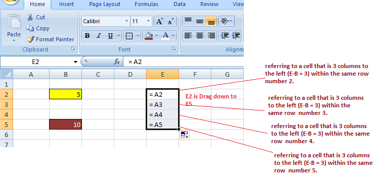
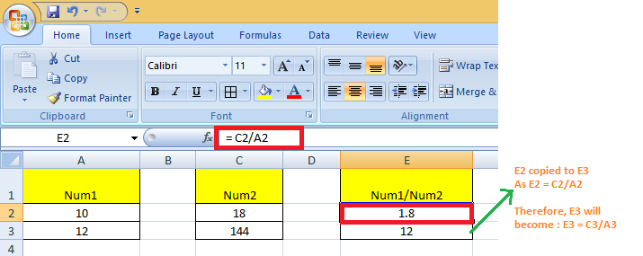
#Example 2:
If you copy the formula = C2 / A2 from the cell “E2” to “E3”, the formula in E3 will automatically become =C3/A3.
When to Use Relative Cell References in Excel
When you need to develop a formula for a set of cells and the formula needs to make a reference to a relative cell reference, relative cell references come in handy.
When this occurs, you can create the formula in one cell and copy it before pasting it into every other cell.
2. Absolute Cell Reference
When copying or using AutoFill, there are times when the cell reference must stay the same. A column and/or row reference is kept constant using dollar signs. So, to get an absolute reference from a relative, we can use the dollar sign ($) characters.
To refer to an actual fixed location on a worksheet whenever copying is done, we use absolute reference. The reference here is locked such that rows and columns do not shift when copied.
How to Use Absolute Cell References in Excel
Below is an example depicting how to use Absolute Cell References in Excel.
#Example:
When we fix both row & column – Say if we want to lock row 2 & column A, we will use $A$2 as:
G2 = C2/$A$2, when copied to G3, G3 becomes = C3/$A$2
Note: C3 is 4 columns left to G3 in the same row.
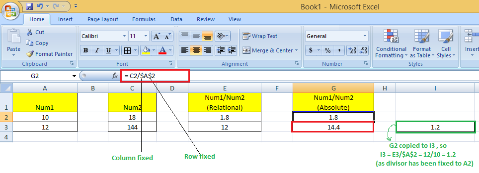
Here, original cell reference A2 is maintained whenever we copy G2 to any of the cells. So I3 = E3/$A$2 because E3 comes from the relative reference (4 columns left to the current one) & /$A$2 comes from the absolute reference.
Therefore, I3 = E3//$A$2 = 12/10 = 1.2
What Does the Dollar ($) Sign Do?
When the row and column numbers are preceded by the dollar symbol ($), it becomes absolute (i.e., stops the row and column number from changing when copied to other cells). Dollar ($) before the row fixes the row & before the column fixes the column.
When to Use Absolute Cell References in Excel
When you don’t want the cell reference to alter when you replicate formulas, absolute cell references come in handy. This can be the situation if you have to use a fixed value in the formula.
3. Mixed Cell Reference
An absolute column and relative row, or an absolute row and relative column, is a mixed cell reference. You get an absolute column or absolute row when you individually put the $ before the column letter or before the row number. Example: $B8 is relative to row 8 but absolute for column B, and B$8 is absolute for row 1 but relative for column A.
Here, the Dollar ($) before the row number fixes/locks the row & before the column name fixes/locks the column.
#Example:
When we fix the only row: If we have G2 = C2/A$2 then :
We used $ before the row number, so we are locking the only row here. When G2 is copied to G3, G3 = C3/A$2 (not C3/A3) because the row has been fixed already.
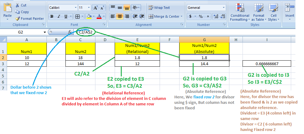
Here, whenever we copy G2 to any other cell, always the divisor will refer to a fixed row 2 (column vary according to the concept of relative reference)
So, when G2 is copied to I3, I3 = E3/C$2 because E3 comes from the relative reference (4 columns left to the current one) & C$2 comes from the absolute reference for row & relative reference for Column (6 Columns left to the current one)
Some Other Ways of Using Cell References With Examples
Now that we are familiar with the basics of using Cell References in Excel, let’s see some other ways of using cell references.
Relative and Absolute Cell References for Calculating Dates
We can use relative and absolute cell references to calculate dates.
Example: To Calculate the Date of Delivery online from the given date of the order placed & no of days it will take to deliver :
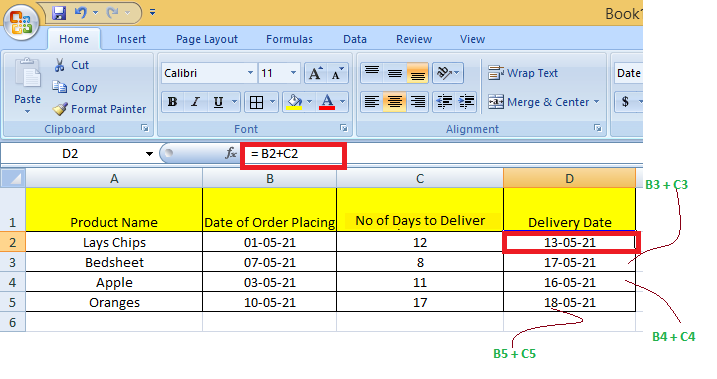
Here, We calculate the Date of Delivery by = Order Date + No of days to deliver. We used Relative cell reference so that individual product delivery dates can be calculated.
Absolute cell references for calculating dates :
Example: To Calculate the Date of Birth When the age is known is a number of days using Current date can be done by making use of absolute reference.
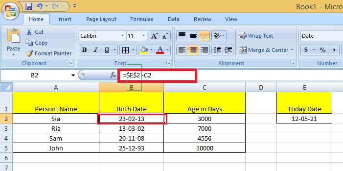
Here, We calculate DOB by = Current Date – Age in days. The Current date is contained in the cell E2 & in subtraction, we fixed that date to subtract from the days.
Whole Column Reference
You will want to refer to all the cells inside a particular column when operating with an Excel worksheet with any number of rows. Simply type a column letter twice with a colon in between to refer to the entire column B, for example, B:B.
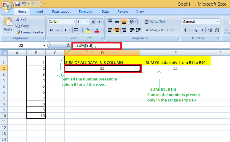
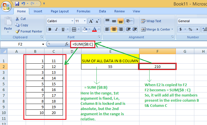
Example: You may want to find the sum of a column of data in certain cases. While you can do this with a regular cell range, such as =SUM(B1:B10), you will need to change the cell range if your spreadsheet grows in size.
Excel, on the other hand, has a cell range that does not require the row number and takes all the cells in the column in action. If you wanted to find the sum of all the values in column B, for example, you would type =SUM (B:B). You can add as much data as you want to your spreadsheet without having to change your cell ranges if you use this type of cell range.
Whole Row Reference
You will want to refer to all the cells inside a particular row when operating with an Excel worksheet with any number of columns. Simply type a row number twice with a colon in between to refer to the entire row, for example, 2:2.
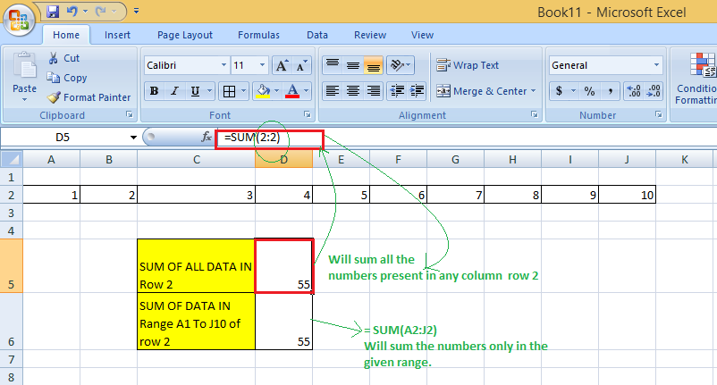
Example: You may want to find the sum of a row of data in certain cases. While you can do this with a regular cell range, such as =SUM(A2 : J2), you will need to change the cell range if your spreadsheet grows in size.
Excel, on the other hand, has a cell range that does not require the column letter and takes all the cells in the row in action. If you wanted to find the sum of all the values in row 2, for example, you would type =SUM (2:2). You can add as much data as you want to your spreadsheet without having to change your cell ranges if you use this type of cell range.
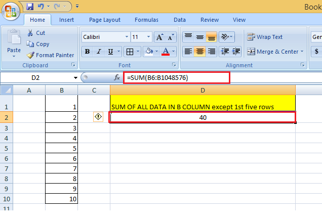
Refer to an Entire Column, Excluding the First Few Rows
To refer to the entire column excluding the first few rows, you need to specify the range as we give in a normal fashion. We know that the Excel worksheets can have only 1,048,576 rows. (To check this, go to an empty cell & press: Ctrl + Down arrow Key)
So, we can do the sum of the entire column B except for the first 5 rows by = SUM(B6:B1048576).
Using a Mixed Entire Column Reference in Excel
You can also create a mixed entire-column reference, say for example $B:B. But, practically, it is difficult to find a situation where it would be used.
Example :
How to switch between Absolute, Relative, and Mixed References
The $ sign can be manually typed in an Excel formula to adjust a relative cell relation to absolute or mixed. You can also speed things up by pressing the F4 key. You must be in formula edit mode to use the F4 shortcut. The steps are :
Firstly, choose the cell that contains the formula. Then, by pressing the F2 key or double-clicking the cell, you can enter Edit mode. Select the cell reference in which you want to make changes. Then, switch between four-cell reference forms by pressing F4.
Example: When you select a cell having only relative reference (i.e., no $ sign), say = B2:
- The first time when you press F4, it becomes =$B$2
- The second time when you press F4, it becomes =B$2
- The third time when you press F4, it becomes=$B2
- The fourth time when you press F4, it becomes back to the relative reference=B2
B2 –Press F4–> =$B$2 –Press F4–> =B$2 –Press F4–> = =$B2 –Press F4–> =B2
So, using F4, you do not require to manually type the $ symbol.
Important Points to Remember
- One of the crucial components for Excel functions or formulas is the cell reference.
- Excel formulas that employ relative cell references automatically change the references to match the correct row and column.
- When copying formulas into non-relative cells, absolute cell references are advised. Excel keeps the absolute cell references constant.
- According to the specifications, a mixed reference only locks one of the references, either the row or the column. Not both are locked.
FAQs on Excel Cell References
1. What are the 3 types of cell references in Excel?
Ans: In Excel, we can use one of three types of cell references:
- Relative Cell References
- Absolute Cell References
- Mixed Cell References

In this lesson we discuss cell references, how to copy or move a formula, and format cells. To begin, let’s clarify what we mean by cell references, which underpin much of the power and versatility of formulas and functions. A concrete grasp on how cell references work will allow you to get the most out of your Excel spreadsheets!
Note: we’re just going to assume that you already know that a cell is one of the squares in the spreadsheet, arranged into columns and rows which are referenced by letters and numbers running horizontally and vertically.
What is a Cell Reference?
A “cell reference” means the cell to which another cell refers. For example, if in cell A1 you have =A2. Then A1 refers to A2.

Let’s review what we said in Lesson 2 about rows and columns so that we can explore cell references further.
Cells in the spreadsheet are referred to by rows and columns. Columns are vertical and labeled with letters. Rows are horizontal and labeled with numbers.
The first cell in the spreadsheet is A1, which means column A, row 1, B3 refers to the cell located on the second column, third row, and so on.
For learning purposes about cell references, we will at times write them as row, column, this is not valid notation in the spreadsheet and is simply meant to make things clearer.
Types of cell references
There are three types of cell references.
Absolute – This means the cell reference stays the same if you copy or move the cell to any other cell. This is done by anchoring the row and column, so it does not change when copied or moved.
Relative – Relative referencing means that the cell address changes as you copy or move it; i.e. the cell reference is relative to its location.
Mixed – This means you can choose to anchor either the row or the column when you copy or move the cell, so that one changes and the other does not. For example, you could anchor the row reference then move a cell down two rows and across four columns and the row reference stays the same. We will explain this further below.
Relative References
Let’s refer to that earlier example – suppose in cell A1 we have a formula that simply says =A2. That means Excel output in cell A1 whatever is inputted into cell A2. In cell A2 we have typed “A2” so Excel displays the value “A2” in cell A1.
Now, suppose we need to make room in our spreadsheet for more data. We need to add columns above and rows to the left, so we have to move the cell down and to the right to make room.
As you move the cell to the right, the column number increases. As you move it down, the row number increases. The cell that it points to, the cell reference, changes as well. This is illustrated below:
Continuing with our example, and looking at the graphic below, if you copy the contents of cell A1 two to the right and four down you have moved it to cell C5.
We copied the cell two columns to the right and four down. This means we have changed the cell it refers two across and four down. A1=A2 now is C5=C6. Instead of referring to A2, now cell C5 refers to cell C6.
The value shown is 0 because cell C6 is empty. In cell C6 we type “I am C6” and now C5 displays “I am C6.”
Example: Text Formula
Let’s try another example. Remember from Lesson 2 where we had to split a full name into first and last name? What happens when we copy this formula?
Write the formula =RIGHT(A3,LEN(A3) – FIND(“,”,A3) – 1) or copy the text to cell C3. Do not copy the actual cell, only the text, copy the text, otherwise it will update the reference.
You can edit the contents of a cell at the top of a spreadsheet in the box next to where is says “fx.” That box is longer than a cell is wide, so it is easier to edit.
Now we have:
Nothing complicated, we have just written a new formula into cell C3. Now copy C3 to cells C2 and C4. Observe the results below:
Now we have Alexander Hamilton and Thomas Jefferson’s first names.
Use the cursor to highlight cells C2, C3, and C4. Point the cursor to cell B2 and paste the contents. Look at what happened – we get an error: “#REF.” Why is this?
When we copied the cells from column C to column B it updated the reference one column to the left =RIGHT(A2,LEN(A2) – FIND(“,”,A2) – 1).
It changed every reference to A2 to the column to the left of A, but there is no column to the left of column A. So the computer does not know what you mean.
The new formula in B2 for example, is =RIGHT(#REF!,LEN(#REF!) – FIND(“,”,#REF!) – 1) and the result is #REF:
Copying a Formula to a Range of Cells
Copying cells is very handy because you can write one formula and copy it to a large area and the reference is updated. This avoids having to edit each cell to ensure it points to the correct place.
By “range” we mean more than one cell. For example, (C1:C10) means all the cells from cell C1 to cell C10. So it is a column of cells. Another example (A1:AZ1) is the top row from column A to column AZ.
If a range cross five columns and ten rows, then you indicate the range by writing the top-left cell and bottom right one, e.g., A1:E10. This is a square area that cross rows and columns and not just part of a column or part of a row.
Here is an example that illustrates how to copy one cell to multiple locations. Suppose we want to show our projected expenses for the month in a spreadsheet so we can make a budget. We make a spreadsheet like this:
Now copy the formula in cell C3 (=B3+C2) to the rest of the column to give a running balance for our budget. Excel updates the cell reference as you copy it. The result is shown below:
As you can see, each new cell updates relative to the new location, so cell C4 updates its formula to =B4 + C3:
Cell C5 updates to =B5 + C4, and so on:
Absolute References
An absolute reference does not change when you move or copy a cell. We use the $ sign to make an absolute reference – to remember that, think of a dollar sign as an anchor.
For example, enter the formula =$A$1 in any cell. The $ in front of the column A means do not change the column, the $ in front of the row 1 means do not change the column when you copy or move the cell to any other cell.
As you can see in the example below, in cell B1 we have a relative reference =A1.When we copy B1 to the four cells below it, the relative reference =A1 changes to the cell to the left, so B2 become A2, B3 become A3, etc. Those cells obviously have no value inputted, so the output is zero.
However, if we use =$A1$1, such as in C1 and we copy it to the four cells below it, the reference is absolute, thus it never changes and the output is always equal to the value in cell A1.
Suppose you are keeping track of your interest, such as in the example below. The formula in C4 = B4 * B1 is the “interest rate” * “balance” = “interest per year.”
Now, you have changed your budget and have saved an additional $2,000 to buy a mutual fund. Suppose it is a fixed rate fund and it pays the same interest rate. Enter the new account and balance into the spreadsheet and then copy the formula = B4 * B1 from cell C4 to cell C5.
The new budget looks like this:
The new mutual fund earns $0 in interest per year, which can’t be right since the interest rate is clearly 5 percent.
Excel highlights the cells to which a formula references. You can see above that the reference to the interest rate (B1) is moved to the empty cell B2. We should have made the reference to B1 absolute by writing $B$1 using the dollars sign to anchor the row and column reference.
Rewrite the first calculation in C4 to read =B4 * $B$1 as shown below:
Then copy that formula from C4 to C5. The spreadsheet now looks like this:
Since we copied the formula one cell down, i.e. increased the row by one, the new formula is =B5*$B$1. The mutual fund interest rate is calculated correctly now, because the interest rate is anchored to cell B1.
This is a good example of when you could use a “name” to refer to a cell. A name is an absolute reference. For example, to assign the name “interest rate” to cell B1, right-click the cell and then select “define name.”
Names can refer to one cell or a range, and you can use a name in a formula, for example =interest_rate * 8 is the same thing as writing =$B$1 * 8.
Mixed References
Mixed references are when either the row or column is anchored.
For example, suppose you are a farmer making a budget. You also own a feed store and sell seeds. You are going to plant corn, soybeans, and alfalfa. The spreadsheet below shows the cost per acre. The “cost per acre” = “price per pound” * “pounds of seeds per acre” – that’s what it will cost you to plant an acre.
Enter the cost per acre as =$B2 * C2 in cell D2. You are saying you want to anchor the price per pound column. Then copy that formula to the other rows in the same column:
Now you want to know the value of your inventory of seeds. You need the price per pound and the number of pounds in inventory to know the value of the inventory.
We add two columns: “pound of seed in inventory” and then “value of inventory.” Now, copy the cell D2 to F4 and note that the row reference in the first part of the original formula ($B2) is updated to row 4 but the column remains fixed because the $ anchors it to “B.”
This is a mixed reference because the column is absolute and the row is relative.
Circular References
A circular reference is when a formula refers to itself.
For example, you cannot write c3 = c3 + 1. This kind of calculation is called “iteration” meaning it repeats itself. Excel does not support iteration because it calculates everything only one time.
If you try do this by typing SUM(B1:B5) in cell B5:
A warning screen pops up:
Excel only tells you that you have a circular reference at the bottom of the screen so you might not notice it. If you do have a circular reference and close a spreadsheet and open it again, Excel will tell you in a pop-up window that you have a circular reference.
If you do have a circular reference, every time you open the spreadsheet, Excel will tell you with that pop-up window that you have a circular reference.
References to Other Worksheets
A “workbook” is a collection of “worksheets.” Simply put, this means you can have multiple spreadsheets (worksheets) in the same Excel file (workbook). As you can see in the example below, our example workbook has many worksheets (in red).
Worksheets by default are named Sheet1, Sheet2, and so forth. You create a new one by clicking the “+” at the bottom of the Excel screen.
You can change the worksheet name to something useful like “loan” or “budget” by right-clicking on the worksheet tab shown at the bottom of the Excel program screen, selecting rename, and typing in a new name.
Or you can simply double-click on the tab and rename it.
The syntax for a worksheet reference is =worksheet!cell. You can use this kind of reference when the same value is used in two worksheets, examples of that might be:
- Today’s date
- Currency conversion rate from Dollars to Euros
- Anything that is relevant to all the worksheets in the workbook
Below is an example of worksheet “interest” making reference to worksheet “loan,” cell B1.
If we look at the “loan” worksheet, we can see the reference to the loan amount:
Coming up Next …
We hope you now have a firm grasp of cell references including relative, absolute, and mixed. There’s certainly a lot.
That’s it for today’s lesson, in Lesson 4, we will discuss some useful functions you may wish to know for daily Excel use.
READ NEXT
- › How to Adjust and Change Discord Fonts
- › This New Google TV Streaming Device Costs Just $20
- › Google Chrome Is Getting Faster
- › HoloLens Now Has Windows 11 and Incredible 3D Ink Features
- › The New NVIDIA GeForce RTX 4070 Is Like an RTX 3080 for $599
- › BLUETTI Slashed Hundreds off Its Best Power Stations for Easter Sale