
For quick access to related information in another file or on a web page, you can insert a hyperlink in a worksheet cell. You can also insert links in specific chart elements.
Note: Most of the screen shots in this article were taken in Excel 2016. If you have a different version your view might be slightly different, but unless otherwise noted, the functionality is the same.
-
On a worksheet, click the cell where you want to create a link.
You can also select an object, such as a picture or an element in a chart, that you want to use to represent the link.
-
On the Insert tab, in the Links group, click Link
 .
.
You can also right-click the cell or graphic and then click Link on the shortcut menu, or you can press Ctrl+K.
-
-
Under Link to, click Create New Document.
-
In the Name of new document box, type a name for the new file.
Tip: To specify a location other than the one shown under Full path, you can type the new location preceding the name in the Name of new document box, or you can click Change to select the location that you want and then click OK.
-
Under When to edit, click Edit the new document later or Edit the new document now to specify when you want to open the new file for editing.
-
In the Text to display box, type the text that you want to use to represent the link.
-
To display helpful information when you rest the pointer on the link, click ScreenTip, type the text that you want in the ScreenTip text box, and then click OK.
 .
.-
On a worksheet, click the cell where you want to create a link.
You can also select an object, such as a picture or an element in a chart, that you want to use to represent the link.
-
On the Insert tab, in the Links group, click Link
.
You can also right-click the cell or object and then click Link on the shortcut menu, or you can press Ctrl+K.
-
-
Under Link to, click Existing File or Web Page.
-
Do one of the following:
-
To select a file, click Current Folder, and then click the file that you want to link to.
You can change the current folder by selecting a different folder in the Look in list.
-
To select a web page, click Browsed Pages and then click the web page that you want to link to.
-
To select a file that you recently used, click Recent Files, and then click the file that you want to link to.
-
To enter the name and location of a known file or web page that you want to link to, type that information in the Address box.
-
To locate a web page, click Browse the Web
, open the web page that you want to link to, and then switch back to Excel without closing your browser.
-
-
If you want to create a link to a specific location in the file or on the web page, click Bookmark, and then double-click the bookmark that you want.
Note: The file or web page that you are linking to must have a bookmark.
-
In the Text to display box, type the text that you want to use to represent the link.
-
To display helpful information when you rest the pointer on the link, click ScreenTip, type the text that you want in the ScreenTip text box, and then click OK.
 , open the web page that you want to link to, and then switch back to Excel without closing your browser.
To link to a location in the current workbook or another workbook, you can either define a name for the destination cells or use a cell reference.
-
To use a name, you must name the destination cells in the destination workbook.
How to name a cell or a range of cells
-
Select the cell, range of cells, or nonadjacent selections that you want to name.
-
Click the Name box at the left end of the formula bar
.
Name box -
In the Name box, type the name for the cells, and then press Enter.
Note: Names can’t contain spaces and must begin with a letter.
-
-
On a worksheet of the source workbook, click the cell where you want to create a link.
You can also select an object, such as a picture or an element in a chart, that you want to use to represent the link.
-
On the Insert tab, in the Links group, click Link
.
You can also right-click the cell or object and then click Link on the shortcut menu, or you can press Ctrl+K.
-
-
Under Link to, do one of the following:
-
To link to a location in your current workbook, click Place in This Document.
-
To link to a location in another workbook, click Existing File or Web Page, locate and select the workbook that you want to link to, and then click Bookmark.
-
-
Do one of the following:
-
In the Or select a place in this document box, under Cell Reference, click the worksheet that you want to link to, type the cell reference in the Type in the cell reference box, and then click OK.
-
In the list under Defined Names, click the name that represents the cells that you want to link to, and then click OK.
-
-
In the Text to display box, type the text that you want to use to represent the link.
-
To display helpful information when you rest the pointer on the link, click ScreenTip, type the text that you want in the ScreenTip text box, and then click OK.
 .
.
 Name box
You can use the HYPERLINK function to create a link that opens a document that is stored on a network server, an intranet, or the Internet. When you click the cell that contains the HYPERLINK function, Excel opens the file that is stored at the location of the link.
Syntax
HYPERLINK(link_location,friendly_name)
Link_location is the path and file name to the document to be opened as text. Link_location can refer to a place in a document — such as a specific cell or named range in an Excel worksheet or workbook, or to a bookmark in a Microsoft Word document. The path can be to a file stored on a hard disk drive, or the path can be a universal naming convention (UNC) path on a server (in Microsoft Excel for Windows) or a Uniform Resource Locator (URL) path on the Internet or an intranet.
-
Link_location can be a text string enclosed in quotation marks or a cell that contains the link as a text string.
-
If the jump specified in link_location does not exist or can’t be navigated, an error appears when you click the cell.
Friendly_name is the jump text or numeric value that is displayed in the cell. Friendly_name is displayed in blue and is underlined. If friendly_name is omitted, the cell displays the link_location as the jump text.
-
Friendly_name can be a value, a text string, a name, or a cell that contains the jump text or value.
-
If friendly_name returns an error value (for example, #VALUE!), the cell displays the error instead of the jump text.
Examples
The following example opens a worksheet named Budget Report.xls that is stored on the Internet at the location named example.microsoft.com/report and displays the text «Click for report»:
=HYPERLINK(«http://example.microsoft.com/report/budget report.xls», «Click for report»)
The following example creates a link to cell F10 on the worksheet named Annual in the workbook Budget Report.xls, which is stored on the Internet at the location named example.microsoft.com/report. The cell on the worksheet that contains the link displays the contents of cell D1 as the jump text:
=HYPERLINK(«[http://example.microsoft.com/report/budget report.xls]Annual!F10», D1)
The following example creates a link to the range named DeptTotal on the worksheet named First Quarter in the workbook Budget Report.xls, which is stored on the Internet at the location named example.microsoft.com/report. The cell on the worksheet that contains the link displays the text «Click to see First Quarter Department Total»:
=HYPERLINK(«[http://example.microsoft.com/report/budget report.xls]First Quarter!DeptTotal», «Click to see First Quarter Department Total»)
To create a link to a specific location in a Microsoft Word document, you must use a bookmark to define the location you want to jump to in the document. The following example creates a link to the bookmark named QrtlyProfits in the document named Annual Report.doc located at example.microsoft.com:
=HYPERLINK(«[http://example.microsoft.com/Annual Report.doc]QrtlyProfits», «Quarterly Profit Report»)
In Excel for Windows, the following example displays the contents of cell D5 as the jump text in the cell and opens the file named 1stqtr.xls, which is stored on the server named FINANCE in the Statements share. This example uses a UNC path:
=HYPERLINK(«\FINANCEStatements1stqtr.xls», D5)
The following example opens the file 1stqtr.xls in Excel for Windows that is stored in a directory named Finance on drive D, and displays the numeric value stored in cell H10:
=HYPERLINK(«D:FINANCE1stqtr.xls», H10)
In Excel for Windows, the following example creates a link to the area named Totals in another (external) workbook, Mybook.xls:
=HYPERLINK(«[C:My DocumentsMybook.xls]Totals»)
In Microsoft Excel for the Macintosh, the following example displays «Click here» in the cell and opens the file named First Quarter that is stored in a folder named Budget Reports on the hard drive named Macintosh HD:
=HYPERLINK(«Macintosh HD:Budget Reports:First Quarter», «Click here»)
You can create links within a worksheet to jump from one cell to another cell. For example, if the active worksheet is the sheet named June in the workbook named Budget, the following formula creates a link to cell E56. The link text itself is the value in cell E56.
=HYPERLINK(«[Budget]June!E56», E56)
To jump to a different sheet in the same workbook, change the name of the sheet in the link. In the previous example, to create a link to cell E56 on the September sheet, change the word «June» to «September.»
When you click a link to an email address, your email program automatically starts and creates an email message with the correct address in the To box, provided that you have an email program installed.
-
On a worksheet, click the cell where you want to create a link.
You can also select an object, such as a picture or an element in a chart, that you want to use to represent the link.
-
On the Insert tab, in the Links group, click Link
.
You can also right-click the cell or object and then click Link on the shortcut menu, or you can press Ctrl+K.
-
-
Under Link to, click E-mail Address.
-
In the E-mail address box, type the email address that you want.
-
In the Subject box, type the subject of the email message.
Note: Some web browsers and email programs may not recognize the subject line.
-
In the Text to display box, type the text that you want to use to represent the link.
-
To display helpful information when you rest the pointer on the link, click ScreenTip, type the text that you want in the ScreenTip text box, and then click OK.
You can also create a link to an email address in a cell by typing the address directly in the cell. For example, a link is created automatically when you type an email address, such as someone@example.com.
You can insert one or more external reference (also called links) from a workbook to another workbook that is located on your intranet or on the Internet. The workbook must not be saved as an HTML file.
-
Open the source workbook and select the cell or cell range that you want to copy.
-
On the Home tab, in the Clipboard group, click Copy.
-
Switch to the worksheet that you want to place the information in, and then click the cell where you want the information to appear.
-
On the Home tab, in the Clipboard group, click Paste Special.
-
Click Paste Link.
Excel creates an external reference link for the cell or each cell in the cell range.

Note: You may find it more convenient to create an external reference link without opening the workbook on the web. For each cell in the destination workbook where you want the external reference link, click the cell, and then type an equal sign (=), the URL address, and the location in the workbook. For example:
=’http://www.someones.homepage/[file.xls]Sheet1′!A1
=’ftp.server.somewhere/file.xls’!MyNamedCell
To select a hyperlink without activating the link to its destination, do one of the following:
-
Click the cell that contains the link, hold the mouse button until the pointer becomes a cross
, and then release the mouse button. -
Use the arrow keys to select the cell that contains the link.
-
If the link is represented by a graphic, hold down Ctrl, and then click the graphic.
 , and then release the mouse button.
You can change an existing link in your workbook by changing its destination, its appearance, or the text or graphic that is used to represent it.
Change the destination of a link
-
Select the cell or graphic that contains the link that you want to change.
Tip: To select a cell that contains a link without going to the link destination, click the cell and hold the mouse button until the pointer becomes a cross
, and then release the mouse button. You can also use the arrow keys to select the cell. To select a graphic, hold down Ctrl and click the graphic.-
On the Insert tab, in the Links group, click Link.
You can also right-click the cell or graphic and then click Edit Link on the shortcut menu, or you can press Ctrl+K.
-
-
In the Edit Hyperlink dialog box, make the changes that you want.
Note: If the link was created by using the HYPERLINK worksheet function, you must edit the formula to change the destination. Select the cell that contains the link, and then click the formula bar to edit the formula.
You can change the appearance of all link text in the current workbook by changing the cell style for links.
-
On the Home tab, in the Styles group, click Cell Styles.
-
Under Data and Model, do the following:
-
To change the appearance of links that have not been clicked to go to their destinations, right-click Link, and then click Modify.
-
To change the appearance of links that have been clicked to go to their destinations, right-click Followed Link, and then click Modify.
Note: The Link cell style is available only when the workbook contains a link. The Followed Link cell style is available only when the workbook contains a link that has been clicked.
-
-
In the Style dialog box, click Format.
-
On the Font tab and Fill tab, select the formatting options that you want, and then click OK.
Notes:
-
The options that you select in the Format Cells dialog box appear as selected under Style includes in the Style dialog box. You can clear the check boxes for any options that you don’t want to apply.
-
Changes that you make to the Link and Followed Link cell styles apply to all links in the current workbook. You can’t change the appearance of individual links.
-
-
Select the cell or graphic that contains the link that you want to change.
Tip: To select a cell that contains a link without going to the link destination, click the cell and hold the mouse button until the pointer becomes a cross
, and then release the mouse button. You can also use the arrow keys to select the cell. To select a graphic, hold down Ctrl and click the graphic. -
Do one or more of the following:
-
To change the link text, click in the formula bar, and then edit the text.
-
To change the format of a graphic, right-click it, and then click the option that you need to change its format.
-
To change text in a graphic, double-click the selected graphic, and then make the changes that you want.
-
To change the graphic that represents the link, insert a new graphic, make it a link with the same destination, and then delete the old graphic and link.
-
-
Right-click the hyperlink that you want to copy or move, and then click Copy or Cut on the shortcut menu.
-
Right-click the cell that you want to copy or move the link to, and then click Paste on the shortcut menu.
By default, unspecified paths to hyperlink destination files are relative to the location of the active workbook. Use this procedure when you want to set a different default path. Each time that you create a link to a file in that location, you only have to specify the file name, not the path, in the Insert Hyperlink dialog box.
Follow one of the steps depending on the Excel version you are using:
-
In Excel 2016, Excel 2013, and Excel 2010:
-
Click the File tab.
-
Click Info.
-
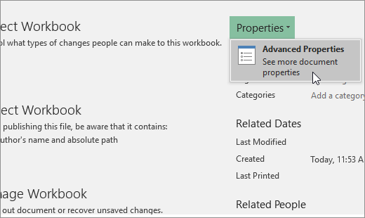
Click Properties, and then select Advanced Properties.
-
In the Summary tab, in the Hyperlink base text box, type the path that you want to use.
Note: You can override the link base address by using the full, or absolute, address for the link in the Insert Hyperlink dialog box.
-
-
In Excel 2007:
-
Click the Microsoft Office Button
, click Prepare, and then click Properties. -
In the Document Information Panel, click Properties, and then click Advanced Properties.
-
Click the Summary tab.
-
In the Hyperlink base box, type the path that you want to use.
Note: You can override the link base address by using the full, or absolute, address for the link in the Insert Hyperlink dialog box.
-
 , click Prepare, and then click Properties.
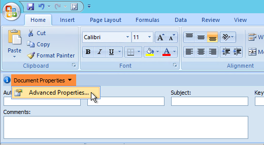
To delete a link, do one of the following:
-
To delete a link and the text that represents it, right-click the cell that contains the link, and then click Clear Contents on the shortcut menu.
-
To delete a link and the graphic that represents it, hold down Ctrl and click the graphic, and then press Delete.
-
To turn off a single link, right-click the link, and then click Remove Link on the shortcut menu.
-
To turn off several links at once, do the following:
-
In a blank cell, type the number 1.
-
Right-click the cell, and then click Copy on the shortcut menu.
-
Hold down Ctrl and select each link that you want to turn off.
Tip: To select a cell that has a link in it without going to the link destination, click the cell and hold the mouse button until the pointer becomes a cross
, and then release the mouse button. -
On the Home tab, in the Clipboard group, click the arrow below Paste, and then click Paste Special.
-
Under Operation, click Multiply, and then click OK.
-
On the Home tab, in the Styles group, click Cell Styles.
-
Under Good, Bad, and Neutral, select Normal.
-
A link opens another page or file when you click it. The destination is frequently another web page, but it can also be a picture, or an email address, or a program. The link itself can be text or a picture.
When a site user clicks the link, the destination is shown in a Web browser, opened, or run, depending on the type of destination. For example, a link to a page shows the page in the web browser, and a link to an AVI file opens the file in a media player.
How links are used
You can use links to do the following:
-
Navigate to a file or web page on a network, intranet, or Internet
-
Navigate to a file or web page that you plan to create in the future
-
Send an email message
-
Start a file transfer, such as downloading or an FTP process
When you point to text or a picture that contains a link, the pointer becomes a hand  , indicating that the text or picture is something that you can click.
What a URL is and how it works
When you create a link, its destination is encoded as a Uniform Resource Locator (URL), such as:
http://example.microsoft.com/news.htm
file://ComputerName/SharedFolder/FileName.htm
A URL contains a protocol, such as HTTP, FTP, or FILE, a Web server or network location, and a path and file name. The following illustration defines the parts of the URL:
1. Protocol used (http, ftp, file)
2. Web server or network location
3. Path
4. File name
Absolute and relative links
An absolute URL contains a full address, including the protocol, the Web server, and the path and file name.
A relative URL has one or more missing parts. The missing information is taken from the page that contains the URL. For example, if the protocol and web server are missing, the web browser uses the protocol and domain, such as .com, .org, or .edu, of the current page.
It is common for pages on the web to use relative URLs that contain only a partial path and file name. If the files are moved to another server, any links will continue to work as long as the relative positions of the pages remain unchanged. For example, a link on Products.htm points to a page named apple.htm in a folder named Food; if both pages are moved to a folder named Food on a different server, the URL in the link will still be correct.
In an Excel workbook, unspecified paths to link destination files are by default relative to the location of the active workbook. You can set a different base address to use by default so that each time that you create a link to a file in that location, you only have to specify the file name, not the path, in the Insert Hyperlink dialog box.
-
On a worksheet, select the cell where you want to create a link.
-
On the Insert tab, select Hyperlink.
You can also right-click the cell and then select Hyperlink… on the shortcut menu, or you can press Ctrl+K.
-
Under Display Text:, type the text that you want to use to represent the link.
-
Under URL:, type the complete Uniform Resource Locator (URL) of the webpage you want to link to.
-
Select OK.
To link to a location in the current workbook, you can either define a name for the destination cells or use a cell reference.
-
To use a name, you must name the destination cells in the workbook.
How to define a name for a cell or a range of cells
Note: In Excel for the Web, you can’t create named ranges. You can only select an existing named range from the Named Ranges control. Alternately, you can open the file in the Excel desktop app, create a named range there, and then access this option from Excel for the web.
-
Select the cell or range of cells that you want to name.
-
On the Name Box box at the left end of the formula bar
, type the name for the cells, and then press Enter.Note: Names can’t contain spaces and must begin with a letter.
-
-
On the worksheet, select the cell where you want to create a link.
-
On the Insert tab, select Hyperlink.
You can also right-click the cell and then select Hyperlink… on the shortcut menu, or you can press Ctrl+K.
-
Under Display Text:, type the text that you want to use to represent the link.
-
Under Place in this document:, enter the defined name or cell reference.
-
Select OK.
When you click a link to an email address, your email program automatically starts and creates an email message with the correct address in the To box, provided that you have an email program installed.
-
On a worksheet, select the cell where you want to create a link.
-
On the Insert tab, select Hyperlink.
You can also right-click the cell and then select Hyperlink… on the shortcut menu, or you can press Ctrl+K.
-
Under Display Text:, type the text that you want to use to represent the link.
-
Under E-mail address:, type the email address that you want.
-
Select OK.
You can also create a link to an email address in a cell by typing the address directly in the cell. For example, a link is created automatically when you type an email address, such as someone@example.com.
You can use the HYPERLINK function to create a link to a URL.
Note: The Link_location can be a text string enclosed in quotation marks or a reference to a cell that contains the link as a text string.
To select a hyperlink without activating the link to its destination, do any of the following:
-
Select a cell by clicking it when the pointer is an arrow.
-
Use the arrow keys to select the cell that contains the link.
You can change an existing link in your workbook by changing its destination, its appearance, or the text that is used to represent it.
-
Select the cell that contains the link that you want to change.
Tip: To select a hyperlink without activating the link to its destination, use the arrow keys to select the cell that contains the link.
-
On the Insert tab, select Hyperlink.
You can also right-click the cell or graphic and then select Edit Hyperlink… on the shortcut menu, or you can press Ctrl+K.
-
In the Edit Hyperlink dialog box, make the changes that you want.
Note: If the link was created by using the HYPERLINK worksheet function, you must edit the formula to change the destination. Select the cell that contains the link, and then select the formula bar to edit the formula.
-
Right-click the hyperlink that you want to copy or move, and then select Copy or Cut on the shortcut menu.
-
Right-click the cell that you want to copy or move the link to, and then select Paste on the shortcut menu.
To delete a link, do one of the following:
-
To delete a link, select the cell and press Delete.
-
To turn off a link (delete the link but keep the text that represents it), right-click the cell and then select Remove Hyperlink.
Need more help?
You can always ask an expert in the Excel Tech Community or get support in the Answers community.
See Also
Remove or turn off links
- Remove From My Forums
-
Question
-
I have an employee who is having trouble linking cells together between documents. The issue occurs when trying to link cells between documents opened from different sources. At first,
I thought it was an issue with hyperthreading, so I had her disable the hyperthreading options within Excel and then I even had her disable hyperthreading on her machine all together, but to no avail. Here is an exmaple:**I open Excel and create a new workbook and then open another workbook using File > Open. When I try to link cells between the two workbooks it works fine and all cells link properly.
**I open Excel and create a new workbook and then open another workbook from a different source (like an e-mail attachment or by double clicking the workbook inside a folder) then when I try to link cells between those two documents, it will not let me. When
I use the link formula (=) in the original workbook then click into the other workbook, it disregards the formula and does not link the cells (Instead of getting a cell surrounded with dotted lines when linking the cell, it stays solid and does not link).What I tested was that Excel was opening two separate instances of itself when opening workbooks from multiple sources, which indeed it was. Hence, I figured disabling hyperthreading would fix this issue. It seems to fix it on MY machine but when my employee
tries this, Excel still poses the same issue.Any thoughts?
Thanks!
Answers
-
Hi Doug,
Could you please try to use Copy and Paste Link
to link the cells?If the file opened is in a Protected View, please click “Enable Editing”.
Then please follow the steps:
- Click the cell that contains the data you want to link to.
- On the Home tab, in the Clipboard group, click Copy
Keyboard shortcut You can also press CTRL+C.
- Click the cell that you want to link from.
- On the Home tab, in the Clipboard group, click Paste
By default, the Paste Options
button appears when you paste copied data.- Click the Paste Options button, and then click Paste Link
Jaynet Zhang
TechNet Community Support

-
Proposed as answer by
Friday, March 16, 2012 12:49 PM
-
Marked as answer by
Jaynet Zhang
Wednesday, March 28, 2012 7:14 AM
Microsoft Excel has a functionality where we can link a textbox to a specific cell. If we change the data in the cell, the value of the linked cell gets updated automatically. Below are the following steps to link a cell to a text box:
1. Open Excel
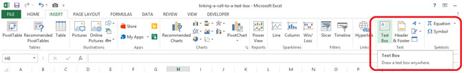
2. Click on the Insert tab
3. Click the Text Box button
4. A text Box will Open

5. Select the Text Box
6. Type = in the Formula Bar
7. Select the cell where you want to give a reference
Let us take an example
1. Open Excel
2. Click on the Insert tab
3. Click the Text Box button
4. A text Box will Open
5. Select the Text Box
6. Type = in the Formula Bar
7. Select the cell A1

8. After we select Cell A1, automatically it will display “=$A$1”
9. Now when we change the Text in cell A1, automatically text in the Text Box will change
This problem is very annoying and not very reasonable: When you sort your Excel table, for example using filters, cell references messed up. Instead of linking to a cell in the same row, they suddenly refer to a cell in a different row. The dangerous part: Often, you want immediately notice it – and something like this might happen… Here is the reason and how to fix broken cell references after sorting data.
Summary
In a hurry? Here is the summary:
- Remove links to own worksheet before sorting an Excel table.
- Find & replace might be the fastest solution here.
Problem: Cell References Broken When Sorting Excel Tables
Admittedly, this is a curious problem. After you sort a table, the cell references within this table are broken.
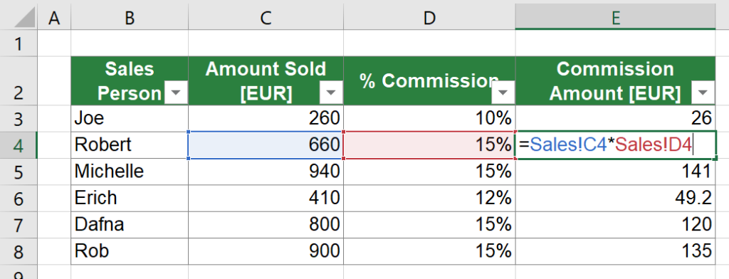
For example, your original table looks like this:
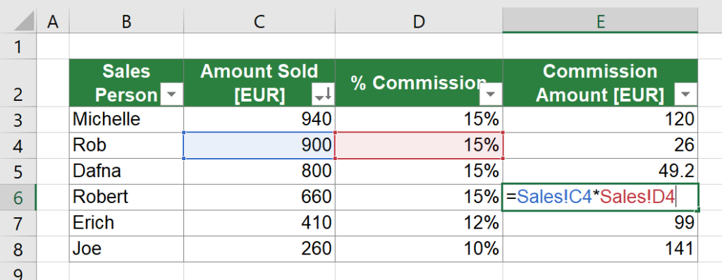
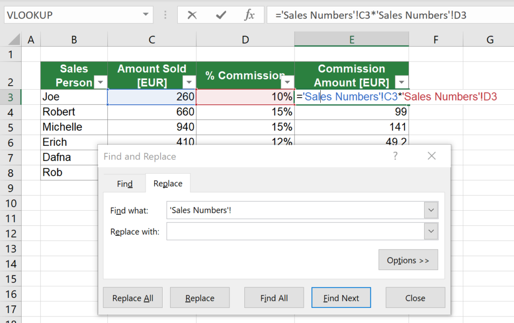
After you have sorted the table by the amount sold in column C, the function for Robert looks like this:
The solution, if cell references are messed up: Remove the worksheet name
The solution for this problem is quite simple: Remove the worksheet name from the cell reference. That way your links will adapt when sorting your table. So, instead of
=Sales!C4*Sales!D4you just write
=C4*D4Sounds simple, right? It has the further advantage that your formula is shorter and easier to follow up.
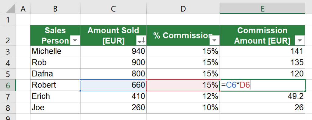
For our example from above, the solution would look like this.
Methods for removing worksheet references from cell links
Method 1: Removing the own sheet name in the reference manually
As usual, deleting the own worksheet name manually might be a fast solution. When you work with tables, you probably just have to do it once and copy & paste your function to all cell in the respective column.
Method 2: Use Find & Replace
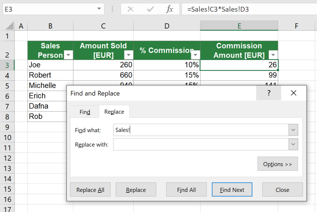
The find & replace function is quite powerful. Open it by pressing Ctrl + H on the keyboard. In the “Find what:” field you search for the worksheet name (in this case “Sales!”) and the “Replace with:” field you leave blank. Make sure to include the exclamation mark.
If something looks broken or you receive error messages after replacing the sheet names, you can undo it by pressing Ctrl + Z on the keyboard.
If your worksheet name includes a space (or any other special character – refer to this article for more information), also replace the ‘ characters. Excel automatically inserts the apostrophes when the sheet name has any of these special characters – and also removes them, when you rename your sheet (for example without spaces).
Method 3: Use Professor Excel Tools
The Excel add-in Professor Excel Tools has a built-in function to clean Excel functions and formulas.
- Select the formulas you want to clean.
- Click on the brush symbol of Professor Excel Tools to open the “Clean Formulas” window.
- Click on start.

This function is included in our Excel Add-In ‘Professor Excel Tools’
(No sign-up, download starts directly)
Image by 412designs from Pixabay

Henrik Schiffner is a freelance business consultant and software developer. He lives and works in Hamburg, Germany. Besides being an Excel enthusiast he loves photography and sports.
-
12-10-2014, 12:19 PM
#1
Registered User
Help! Excel not linking cells correctly after drag down?
So i have a database of emails and I am trying to merge them in sets of 10, spaced by a semicolon. I have the formula:
=G1&»;»&G2&»;»&G3&»;»&G4&»;»&G5&»;»&G6&»;»&G7&»;»&G8&»;»&G9&»;»&G10
however when I drag down this is what the next set of ten become:
=G2&»;»&G3&»;»&G4&»;»&G5&»;»&G6&»;»&G7&»;»&G8&»;»&G9&»;»&G10&»;»&G11
I have a ton of emails and I cannot go through all of them and change all of the individual sets, someone please help!
extra:
also some of the cells in my database are blank, and if they are it adds an extra ;; within the new cell…. is there anyway to avoid that?
-
12-10-2014, 01:01 PM
#2
Re: Help! Excel not linking cells correctly after drag down?
You have not explained in enough detail. Based on how relative references work (see this overview of references in formulas https://support.office.com/en-us/art…es_in_formulas ), this sounds like correct, normal behavior if you copy that formula down one cell. In order for us to suggest something other than «normal» behavior for copying functions, we will need to know what is incorrect about Excel’s default behavior and exactly what you want the copied formula to do instead.
Originally Posted by shgMathematics is the native language of the natural world. Just trying to become literate.
-
12-10-2014, 01:06 PM
#3
Re: Help! Excel not linking cells correctly after drag down?
You cannot drag the formula down 1 row, and expect the reference to jump 10 rows.
=G1 copied down 1 row becomes =G2 not G11I will see what I can put together for you
1. Use code tags for VBA. [code] Your Code [/code] (or use the # button)
2. If your question is resolved, mark it SOLVED using the thread tools
3. Click on the star if you think someone helped youRegards
Ford
-
12-10-2014, 01:11 PM
#4
Re: Help! Excel not linking cells correctly after drag down?
OK use your formula for the 1st 1, then use this below it, copied down…
-
12-10-2014, 01:34 PM
#5
Re: Help! Excel not linking cells correctly after drag down?
-
12-10-2014, 01:50 PM
#6
Re: Help! Excel not linking cells correctly after drag down?
if you are interested in Vba code then here is the possible short solution.
Before trying above formula, Copy the following Code and paste in the Alt + F11 window after inserting a module.
I hope this will do the job.
Regards,
Vikas Gautam
Excel-buzz.blogspot.com
Excel is not a matter of Experience, its a matter of Application.
Say Thanks, Click * Add Reputation

