
Excel for Microsoft 365 Excel for Microsoft 365 for Mac Excel 2021 Excel 2021 for Mac Excel 2019 Excel 2019 for Mac Excel 2016 Excel 2016 for Mac Excel 2013 Excel 2010 Excel 2007 Excel for Mac 2011 More…Less
Apply number formats such as dates, currency, or fractions to cells in a worksheet. For example, if you’re working on your quarterly budget, you can use the Currency number format so your numbers represent money. Or, if you have a column of dates, you can specify that you want the dates to appear as March 14, 2012, 14-Mar-12, or 3/14.
Follow these steps to format numbers:
-
Select the cells containing the numbers you need to format.
-
Select CTRL+1.
On a Mac, select Control+1, or Command+1.
-
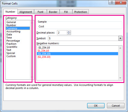
In the window that displays, select the Number tab (skip this step if you’re using Microsoft 365 for the web).
-
Select a Category option, and then select specific formatting changes on the right.

Tip: Do you have numbers showing up in your cells as #####? This probably means your cell isn’t wide enough to show the whole number. Try double-clicking the right border of the column that contains the cells with #####. This will change the column width and row height to fit the number. You can also drag the right border of the column to make it any size you want.
Stop your numbers from automatically formatting
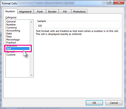
Sometimes if you enter numbers into a cell—or import them from another data source—Excel doesn’t format them as you expect. If, for example, you type a number along with a slash mark (/) or a hyphen (-), Excel might apply a Date format. You can prevent this automatic number formatting by applying the Text format to the cells.
It’s easy to do:
-
Select the cells that contain numbers you don’t want Excel to automatically format.
-
Select CTRL+1.
On a Mac, select Control+1, or Command+1.
-
On the Number tab, select Text in the Category list.
Need more help?
You can always ask an expert in the Excel Tech Community or get support in the Answers community.
See Also
Format a date the way you want
Format numbers as percentages
Format negative percentages to make them easy to find
Format numbers as currency
Create a custom number format
Convert dates stored as text to dates
Fix text-formatted numbers by applying a number format
Need more help?
Introduction
Number formats control how numbers are displayed in Excel. The key benefit of number formats is that they change how a number looks without changing any data. They are a great way to save time in Excel because they perform a huge amount of formatting automatically. As a bonus, they make worksheets look more consistent and professional.
Video: What is a number format
What can you do with custom number formats?
Custom number formats can control the display of numbers, dates, times, fractions, percentages, and other numeric values. Using custom formats, you can do things like format dates to show month names only, format large numbers in millions or thousands, and display negative numbers in red.

Where can you use custom number formats?
Many areas in Excel support number formats. You can use them in tables, charts, pivot tables, formulas, and directly on the worksheet.
- Worksheet — format cells dialog
- Pivot Tables — via value field settings
- Charts — data labels and axis options
- Formulas — via the TEXT function
What is a number format?
A number format is a special code to control how a value is displayed in Excel. For example, the table below shows 7 different number formats applied to the same date, January 1, 2019:
| Input | Code | Result |
|---|---|---|
| 1-Jan-2019 | yyyy | 2019 |
| 1-Jan-2019 | yy | 19 |
| 1-Jan-2019 | mmm | Jan |
| 1-Jan-2019 | mmmm | January |
| 1-Jan-2019 | d | 1 |
| 1-Jan-2019 | ddd | Tue |
| 1-Jan-2019 | dddd | Tuesday |
The key thing to understand is that number formats change the way numeric values are displayed, but they do not change the actual values.
Where can you find number formats?
On the home tab of the ribbon, you’ll find a menu of build-in number formats. Below this menu to the right, there is a small button to access all number formats, including custom formats:

This button opens the Format Cells dialog box. You’ll find a complete list of number formats, organized by category, on the Number tab:

Note: you can open Format Cells dialog box with the keyboard shortcut Control + 1.
General is default
By default, cells start with the General format applied. The display of numbers using the General number format is somewhat «fluid». Excel will display as many decimal places as space allows, and will round decimals and use scientific number format when space is limited. The screen below shows the same values in column B and D, but D is narrower and Excel makes adjustments on the fly.

How to change number formats
You can select standard number formats (General, Number, Currency, Accounting, Short Date, Long Date, Time, Percentage, Fraction, Scientific, Text) on the home tab of the ribbon using the Number Format menu.
Note: As you enter data, Excel will sometimes change number formats automatically. For example if you enter a valid date, Excel will change to «Date» format. If you enter a percentage like 5%, Excel will change to Percentage, and so on.
Shortcuts for number formats
Excel provides a number of keyboard shortcuts for some common formats:
| Format | Shortcut |
|---|---|
| General format | Ctrl Shift ~ |
| Currency format | Ctrl Shift $ |
| Percentage format | Ctrl Shift % |
| Scientific format | Ctrl Shift ^ |
| Date format | Ctrl Shift # |
| Time format | Ctrl Shift @ |
| Custom formats | Control + 1 |
See also: 222 Excel Shortcuts for Windows and Mac
Where to enter custom formats
At the bottom of the predefined formats, you’ll see a category called custom. The Custom category shows a list of codes you can use for custom number formats, along with an input area to enter codes manually in various combinations.

When you select a code from the list, you’ll see it appear in the Type input box. Here you can modify existing custom code, or to enter your own codes from scratch. Excel will show a small preview of the code applied to the first selected value above the input area.
Note: Custom number formats live in a workbook, not in Excel generally. If you copy a value formatted with a custom format from one workbook to another, the custom number format will be transferred into the workbook along with the value.
How to create a custom number format
To create custom number format follow this simple 4-step process:
- Select cell(s) with values you want to format
- Control + 1 > Numbers > Custom
- Enter codes and watch preview area to see result
- Press OK to save and apply
Tip: if you want base your custom format on an existing format, first apply the base format, then click the «Custom» category and edit codes as you like.
How to edit a custom number format
You can’t really edit a custom number format per se. When you change an existing custom number format, a new format is created and will appear in the list in the Custom category. You can use the Delete button to delete custom formats you no longer need.
Warning: there is no «undo» after deleting a custom number format!
Structure and Reference
Excel custom number formats have a specific structure. Each number format can have up to four sections, separated with semi-colons as follows:

This structure can make custom number formats look overwhelmingly complex. To read a custom number format, learn to spot the semi-colons and mentally parse the code into these sections:
- Positive values
- Negative values
- Zero values
- Text values
Not all sections required
Although a number format can include up to four sections, only one section is required. By default, the first section applies to positive numbers, the second section applies to negative numbers, the third section applies to zero values, and the fourth section applies to text.
- When only one format is provided, Excel will use that format for all values.
- If you provide a number format with just two sections, the first section is used for positive numbers and zeros, and the second section is used for negative numbers.
- To skip a section, include a semi-colon in the proper location, but don’t specify a format code.
Characters that display natively
Some characters appear normally in a number format, while others require special handling. The following characters can be used without any special handling:
| Character | Comment |
|---|---|
| $ | Dollar |
| +- | Plus, minus |
| () | Parentheses |
| {} | Curly braces |
| <> | Less than, greater than |
| = | Equal |
| : | Colon |
| ^ | Caret |
| ‘ | Apostrophe |
| / | Forward slash |
| ! | Exclamation point |
| & | Ampersand |
| ~ | Tilde |
| Space character |
Escaping characters
Some characters won’t work correctly in a custom number format without being escaped. For example, the asterisk (*), hash (#), and percent (%) characters can’t be used directly in a custom number format – they won’t appear in the result. The escape character in custom number formats is the backslash (). By placing the backslash before the character, you can use them in custom number formats:
| Value | Code | Result |
|---|---|---|
| 100 | #0 | #100 |
| 100 | *0 | *100 |
| 100 | %0 | %100 |
Placeholders
Certain characters have special meaning in custom number format codes. The following characters are key building blocks:
| Character | Purpose |
|---|---|
| 0 | Display insignificant zeros |
| # | Display significant digits |
| ? | Display aligned decimals |
| . | Decimal point |
| , | Thousands separator |
| * | Repeat following character |
| _ | Add space |
| @ | Placeholder for text |
Zero (0) is used to force the display of insignificant zeros when a number has fewer digits than zeros in the format. For example, the custom format 0.00 will display zero as 0.00, 1.1 as 1.10 and .5 as 0.50.

Pound sign (#) is a placeholder for optional digits. When a number has fewer digits than # symbols in the format, nothing will be displayed. For example, the custom format #.## will display 1.15 as 1.15 and 1.1 as 1.1.

Question mark (?) is used to align digits. When a question mark occupies a place not needed in a number, a space will be added to maintain visual alignment.

Period (.) is a placeholder for the decimal point in a number. When a period is used in a custom number format, it will always be displayed, regardless of whether the number contains decimal values.
Comma (,) is a placeholder for the thousands separators in the number being displayed. It can be used to define the behavior of digits in relation to the thousands or millions digits.

Asterisk (*) is used to repeat characters. The character immediately following an asterisk will be repeated to fill remaining space in a cell.

Underscore (_) is used to add space in a number format. The character immediately following an underscore character controls how much space to add. A common use of the underscore character is to add space to align positive and negative values when a number format is adding parentheses to negative numbers only. For example, the number format «0_);(0)» is adding a bit of space to the right of positive numbers so that they stay aligned with negative numbers, which are enclosed in parentheses.

At (@) — placeholder for text. For example, the following number format will display text values in blue:
0;0;0;[Blue]@
See below for more information about using color.
Automatic rounding
It’s important to understand that Excel will perform «visual rounding» with all custom number formats. When a number has more digits than placeholders on the right side of the decimal point, the number is rounded to the number of placeholders. When a number has more digits than placeholders on the left side of the decimal point, extra digits are displayed. This is a visual effect only; actual values are not modified.
Number formats for TEXT
To display both text along with numbers, enclose the text in double quotes («»). You can use this approach to append or prepend text strings in a custom number format, as shown in the table below.
| Value | Code | Result |
|---|---|---|
| 10 | General» units» | 10 units |
| 10 | 0.0″ units» | 10.0 units |
| 5.5 | 0.0″ feet» | 5.5 feet |
| 30000 | 0″ feet» | 30000 feet |
| 95.2 | «Score: «0.0 | Score: 95.2 |
| 1-Jun | «Date: «mmmm d | Date: June 1 |
Number formats for DATES
Dates in Excel are just numbers, so you can use custom number formats to change the way they display. Excel has many specific codes you can use to display components of a date in different ways. The screen below shows how Excel displays the date in D5, September 3, 2018, with a variety of custom number formats:

Number formats for TIME
Times in Excel are fractional parts of a day. For example, 12:00 PM is 0.5, and 6:00 PM is 0.75. You can use the following codes in custom time formats to display components of a time in different ways. The screen below shows how Excel displays the time in D5, 9:35:07 AM, with a variety of custom number formats:

Note: m and mm can’t be used alone in a custom number format since they conflict with the month number code in date format codes.
Number formats for ELAPSED TIME
Elapsed time is a special case and needs special handling. By using square brackets, Excel provides a special way to display elapsed hours, minutes, and seconds. The following screen shows how Excel displays elapsed time based on the value in D5, which represents 1.25 days:

Number formats for COLORS
Excel provides basic support for colors in custom number formats. The following 8 colors can be specified by name in a number format: [black] [white] [red][green] [blue] [yellow] [magenta] [cyan]. Color names must appear in brackets.

Colors by index
In addition to color names, it’s also possible to specify colors by an index number (Color1,Color2,Color3, etc.) The examples below are using the custom number format: [ColorX]0″▲▼», where X is a number between 1-56:
[Color1]0"▲▼" // black
[Color2]0"▲▼" // white
[Color3]0"▲▼" // red
[Color4]0"▲▼" // green
etc.
The triangle symbols have been added only to make the colors easier to see. The first image shows all 56 colors on a standard white background. The second image shows the same colors on a gray background. Note the first 8 colors shown correspond to the named color list above.


Apply number formats in a formula
Although most number formats are applied directly to cells in a worksheet, you can also apply number formats inside a formula with the TEXT function. For example, with a valid date in A1, the following formula will display the month name only:
=TEXT(A1,"mmmm")
The result of the TEXT function is always text, so you are free to concatenate the result of TEXT to other strings:
="The contract expires in "&TEXT(A1,"mmmm")
The screen below shows the number formats in column C being applied to numbers in column B using the TEXT function:

One quirk of the TEXT function relates to double quotes («») that are part of certain custom number formats. Because the format_text is entered as a text string, Excel won’t allow you to enter the formula without removing the quotes or adding more quotes. For example, to display a large number in thousands, you can use a custom number format like this:
0, "k"Notice k appears in quotes («k»). To apply the same format with the TEXT function, you can use simply:
=TEXT(A1,"0, k")Notice the k is not surrounded by quotes. Alternately, you can add extra double quotes as below, which returns the same result:
=TEXT(A1,"0,""K""")This behavior only occurs when you are hardcoding a format inside TEXT. If you are applying a format entered elsewhere on the worksheet (as in cells C6 and C9 in the worksheet above) you can use a standard number format.
Measurements
You can use a custom number format to display numbers with an inches mark («) or a feet mark (‘). In the screen below, the number formats used for inches and feet are:
0.00 ' // feet
0.00 " // inches

These results are simplistic, and can’t be combined in a single number format. You can however use a formula to display feet together with inches.
Conditionals
Custom number formats also up to two conditions, which are written in square brackets like [>100] or [<=100]. When you use conditionals in custom number formats, you override the standard [positive];[negative];[zero];[text] structure. For example, to display values below 100 in red, you can use:
[Red][<100]0;0
To display values greater than or equal to 100 in blue, you can extend the format like this:
[Red][<100]0;[Blue][>=100]0

To apply more than two conditions, or to change other cell attributes, like fill color, etc. you’ll need to switch to Conditional Formatting, which can apply formatting with much more power and flexibility using formulas.
Plural text labels
You can use conditionals to add an «s» to labels greater than zero with a custom format like this:
[=1]0″ day»;0″ days»

Telephone numbers
Custom number formats can also be used for telephone numbers, as shown in the screen below:

Notice the third and fourth examples use a conditional format to check for numbers that contain an area code. If you have data that contains phone numbers with hard-coded punctuation (parentheses, hyphens, etc.) you will need to clean the telephone numbers first so that they only contain numbers.
Hide all content
You can actually use a custom number format to hide all content in a cell. The code is simply three semi-colons and nothing else ;;;
To reveal the content again, you can use the keyboard shortcut Control + Shift + ~, which applies the General format.
Other resources
- Developer Bryan Braun built a nice interactive tool for building custom number formats
Option 1: Change the column formatting from Text to General by multiplying the numbers by 1:
1. Enter the number 1 into a cell and copy it.
2. Select the column formatted as text, press Shift+F10 or right-click, and then select Paste Special from the shortcut menu.
3. Select the Multiply option button in the Paste Special dialog box, and then click OK.
Option 2: Change the column formatting from Text to General using the Text to Columns technique:
1. Select the column formatted as text.
2. From the Data menu, select Text to Columns.
3. In Step 1 of 3, select the Fixed width option button.
4. Skip Step 2 of 3.
5. In Step 3 of 3, select the General option button in the Column data format section, and then click Finish.
Screenshot // Problem: Values Not Formatting as Numbers

![]()

![]()

If you used Excel in any shape or form, there is a pretty good chance that you’ve used the formatting and number formatting features. Formatting options like number, currency, percentage, date and time values are easily accessible to users. However, that’s not all there is in the world of text and number formatting. Going down the rabbit hole, custom formatting can help you fully configure Excel’s built-in settings for formatting.
The main advantage of this approach is that you can alter the look of your data without changing the actual values. This means that you do not need to use additional spaces or formulas to create the layout you want and preserve the raw data.
If you want to modify your data anyways, or need to change a value inside a formula, you can use the TEXT function with all custom formatting syntax we are going to cover in this article. It should be noted that the TEXT function returns a text, and the return value cannot be used in mathematical calculations. If you do, you will receive a #VALUE! error. In this article we’re going to be using a workbook template. You can download it below.
How to create a custom number format in Excel
- Select the cell to be formatted and press Ctrl+1 to open the Format Cells dialog. An alternative way to do is by right-clicking the cell and then going to Format Cells > Number Tab.
- Under Category, select Custom.
- Type in the format code into the Type
- Click OK to save your changes.
Note: In Format Cells dialog you can modify the built-in format codes by selecting the format you want to modify in its own category (i.e. Currency > ($1,234.10)) and then selecting Custom Category. Don’t worry, Excel will not let you delete built-in formats.

Basics
Syntax
The format code has 4 sections separated by semicolons.
POSITIVE; NEGATIVE; ZERO; TEXT
These sections are optional,
- If a code contains only 1 section, the format is applied to all number types — positive, negative and zero.
- If a code contains 2 sections, the first section is used for positive and zero values, while the second section is applied to negative values.
- If a code contains 3 sections, the first is for positive, the second is for negative, and the third is for zero.
- A code only affects text values if all sections exist.
Default format type in Excel is called General. You can type General for sections you don’t want formatted. Make sure you use a minus sign (-) with General if you want to skip negative values.
If you want to completely hide a type, leave it blank after the semicolon. For example; to hide 0 values, General;-General;;General
Placeholders and the Cheat Sheet
| Placeholder | Description | Raw Value | Format Code | Formatted Value |
| General | Default format | 1234.567 | General | 1234.567 |
| # | Placeholder for digits (numbers) and does not add any leading zeroes. | 1234.567 | #####.#### | 1234.567 |
| 0 | Placeholder for digits (numbers) and add any leading zeroes. | 1234.567 | 00000.0000 | 01234.5670 |
| ? | Placeholder for digits (numbers) and add space characters. | 1234.567 | ?????.???? | 1234.567 |
| . | Placeholder for the decimal place. | 1234.567 | 0.00 | 1234.57 |
| _ | Adds a blank space, to the width of the following character. You can use in combination with parentheses to add left and right indents, _( and _) respectively. | 99 | _(#_);(#) | 99 |
| -25 | (25) | |||
| 58 | 58 | |||
| 12 | 12 | |||
| -71 | (71) | |||
| 36 | 36 | |||
| * | Repeats the character after asterisk until the width of the cell is filled. | 66 | 0 *! | 66 !!!!!!!!!!!!!!! |
| Full Name | @ *_ | Full Name ____ | ||
| % | Convert value to a percentage with % sign | 0.12 | % | 12% |
| , | Thousands separator | 1234.567 | #, | 1 |
| 12345678 | #, | 12,346 | ||
| 12345678 | #,###, | 12,346 | ||
| 12345678 | #,, | 12 | ||
| E | Scientific notation format. Requires a ‘+’ symbol after, and a digit placeholder before and after. | 1234.567 | 0.00E+00 | 1.23E+03 |
| / | Represents fractions | 1.234 | # ##/## | 1 11/47 |
| 1.234 | # 000/000 | 1 117/500 | ||
| 1.234 | ##/## | 58/47 | ||
| «» | Text placeholder for multiple characters | 1234.567 | #,##0 «km/h» | 1,235 km/h |
| Good | «Result is: «@ | Result is: Good | ||
| Text placeholder for single character | 1234 | #.00, K | 1.23 K | |
| 1234567 | #.00,, M | 1.23 M | ||
| @ | Placeholder for text | Bad | «Result is: «@ | Result is: Bad |
| [color] | Change Color of value. Options: [Black], [Green], [White], [Blue], [Magenta], [Yellow], [Cyan], [Red] | 1234.567 | [Green]#,##0.00_); [Red](#,##0.00); [Blue]0.00_); [Magenta]@ |
1,234.57 |
| -1234.567 | (1,234.57) | |||
| 0 | 0.00 | |||
| This is a text | This is a text |
Common Practices
Display and control of the first digit and decimals
Decimal places in the code are indicated with a period (.). Number of zeroes after the period (.) define the number of decimal places. For example,
- 0 — display 1 decimal place
- 00 — display 2 decimal places
If the number has more decimals than the decimal placeholders defined, the number will be rounded to the nearest number of placeholders.
| Raw Value | Format Code | Formatted Value |
| 123.4 | 0.0 | 123.4 |
| 123.4 | 0.00 | 123.40 |
| 123.45 | 0.00 | 123.45 |
| 123.45 | 0.00 | 123.46 |
| 123.456 | 0.0 | 123.5 |
Alternatively, hash (#) and question mark (?) symbols can be used as decimal places. However, because any missing decimal places will be filled with zeroes, using zeroes instead will be easier to read.
| Raw Value | Format Code | Formatted Value |
| 0.25 | 0.00 | 0.25 |
| 0.25 | #.## | .25 |
| 123 | 0.00 | 123.0 |
| 123 | #.?? | 123.00 |
| 123 | #.## | 123. |
Add text to numbers
Custom text can be added to the beginning or the end of a value. Text and characters should be added inside quotes («») and backslashes (). You can use backslash () to add single character.
| Raw Value | Format Code | Formatted Value |
| 123.4 | 0.0 «ft.» | 123.4 ft. |
| 123.4 | 0.00 l | 123.40 l |
| 123.45 | «Approx.» 0 | Approx. 123 |
| 123.45 | «Result:» 0.00 C | Result: 123.46 C |
| Bad | «Result is: «@ | Result is: Bad |
Quotation marks or backslashes are not necessary for spaces ( ) and some special characters.
| Symbol | Description |
| + and — | Plus and minus signs |
| ( ) | Left and right parenthesis |
| : | Colon |
| ^ | Caret |
| ‘ | Apostrophe |
| { } | Curly brackets |
| < > | Less-than and greater than signs |
| = | Equal sign |
| / | Forward slash |
| ! | Exclamation point |
| & | Ampersand |
| ~ | Tilde |
| Space character |
Below are some special characters you can use by copying or typing in the numerical code while pressing down Alt button.
| Symbol | Code | Description |
| ™ | Alt+0153 | Trademark |
| © | Alt+0169 | Copyright symbol |
| ° | Alt+0176 | Degree symbol |
| ± | Alt+0177 | Plus-Minus sign |
| µ | Alt+0181 | Micro sign |
Hide value
If you leave any number of sections blank, the value of those sections will be hidden. A section should always be separated (defined) by a semicolon (;). Here are some examples,
| Raw Value | Format Code | Formatted Value |
| 1 | 0;;0; | 1 |
| -2 | 0;;0; | |
| 0 | 0;;0; | 0 |
| Some text | 0;;0; | |
| 1 | ;(0);;@ | |
| -2 | ;(0);;@ | (2) |
| 0 | ;(0);;@ | |
| Some text | ;(0);;@ | Some Text |
| 1 | ;;; | |
| -2 | ;;; | |
| 0 | ;;; | |
| Some text | ;;; |
Replace zeroes with dashes
Zeroes can make data tables look more complicated than they actually are. You can hide them completely by using the previous method, or replace them with any character of your choice. Dash (-) is a common example. All you need to is place a dash into the ‘Zero section’.
| Raw Value | Format Code | Formatted Value |
| 0 | General;-General;»-«;General | — |
| 3487 | General;-General;»-«;»-« | — |
| 12 | #,##0.00;(#,##0.00);»-«; | — |
Start with zeroes
If try to enter a ZIP number that starts with 0, the leading zeroes will be removed automatically by Excel. To keep the leading zeros, use zero (0) placeholder for whole numbers.
| Raw Value | Format Code | Formatted Value |
| 10010 | 00000 | 10010 |
| 3487 | 00000 | 03487 |
| 12 | 00000 | 00012 |
| 0 | 00000 | 00000 |
| 123456 | 00000 | 123456 |
Dealing with thousands, millions, and more
You may have noticed that ‘0.0’ or other simple formats do not separate thousands or millions. Adding a comma into the code will insert commas to separate numbers.
| Raw Value | Format Code | Formatted Value |
| 1234 | #,##0 | 1,234 |
| 123456 | #,##0 | 123,456 |
| 12345678 | #,##0 | 12,345,678 |
| 123456.789 | #,##0 | 123,457 |
| 123456.789 | #,##0.0 | 123,456.8 |
There must be placeholders for numbers smaller than one thousand, otherwise such values will be hidden. This behavior allows us to round and format our value to show only thousands or millions.
| Raw Value | Format Code | Formatted Value |
| 1234 | #, | 1 |
| 123456 | #, | 123 |
| 12345678 | #, | 12345 |
| 12345678 | #,, | 12 |
| 123456 | #.0, K | 123.5 K |
| 12345678 | #.0,, M | 12.3 M |
Display numbers as phone numbers
Phone numbers can be hard to read without any separators. Custom Number Format Codes is perfect for this job. The hash (#) character should be your best bet to avoid any redundancy of placeholders (0, ?)
| Raw Value | Format Code | Formatted Value |
| 1234567890 | (###) ###-#### | (123) 456-7890 |
| 12345678900 | (###) #### #### | (123) 4567 8900 |
| 1234567890 | (##) #### #### | (12) 3456 7890 |
Showing Month and Weekday Names
Date and time values are stored as numbers in Excel. When you enter a date, Excel automatically converts it into a numerical value, and then formats the cell.
Before jumping into the code, let’s review some basics. Formatting code has special placeholders for date and time formatting that behave a bit differently. For example, while m and mm will show month as a number, mmm and mmmm will show as a text string. Below are some examples.
| Raw Value | Format Code | Formatted Value |
| 4/1/2018 | m | 4 |
| 4/1/2018 | mm | 04 |
| 4/1/2018 | mmm | Apr |
| 4/1/2018 | mmmm | April |
| 4/1/2018 | mmmmm | A |
| 4/1/2018 | d | 1 |
| 4/1/2018 | dd | 01 |
| 4/1/2018 | ddd | Sun |
| 4/1/2018 | dddd | Sunday |
| 4/1/2018 11:59:31 PM | dddd, mmmm dd, yyyy h:mm AM/PM;@ | Sunday, April 01, 2018 11:59 PM |
Here is the full list of options for the date 4/1/2018 23:59:31 ,
| Format Code | Description | Example (4/1/2018 23:59:31) |
| yyyy | Displays the year as a four-digit number. | 2018 |
| yy | Displays the year as a two-digit number. | 18 |
| m | Displays the month as a number without a leading zero. | 4 |
| mm | Displays the month with a leading zero. | 04 |
| mmm | Displays the month as text, as an abbreviation. | Apr |
| mmmm | Displays the month as text. | April |
| mmmmm | Displays the month as a single character | A |
| d | Displays the day as a number, without a leading zero. | 1 |
| dd | Displays the day as a number, with a leading zero. | 01 |
| ddd | Displays the day as a day of the week, as an abbreviation. | Sun |
| dddd | Displays the day as a day of the week, without abbreviation | Sunday |
| h | Displays the hour without a leading zero. | 23 |
| hh | Displays the hour with a leading zero. | 23 |
| [h] | Displays elapsed time in hours (to be used when the time value exceeds 24 hours). | 1036607 |
| m | Displays the minute without a leading zero. | 4 |
| mm | Displays the minute with a leading zero. | 04 |
| [m] | Displays elapsed time in minutes (to be used when the time value exceeds 60 minutes). | 62196479 |
| s | Displays the second without a leading zero. | 31 |
| ss | with a leading zero. | 31 |
| [s] | Displays elapsed time in seconds (to be used when the time value exceeds 60 seconds). | 3731788771 |
| AM/PM | Converts to 12-hour time. Displays either AM/am/A/a or PM/pm/P/p depending on the time of day. | PM |
| am/pm | pm | |
| A/P | P | |
| a/p | p |
Come in Colors Everywhere
Number Formatting can be used color sections of a code. A common example is using the color red for negative numbers. Color code must be placed inside square brackets (i.e. [color]), and entered at the beginning of a section. Here are some available colors,
- [Black]
- [Blue]
- [Cyan]
- [Green]
- [Magenta]
- [Red]
- [White]
- [Yellow]
| Raw Value | Format Code | Formatted Value |
| 1234.567 | [Green]#,##0.00_);[Red](#,##0.00);[Blue]0.00);[Magenta]@ | 1,234.57 |
| -1234.567 | (1,234.57) | |
| 0 | 0.00 | |
| This is a text | This is a text |
Conditions
Although Excel has conditional formatting menu, basic conditions can be applied through code. Condition should be placed inside square brackets (i.e. [condition]) just like colors. Conditions are similar to the conditions in some functions (i.e. SUMIF). First add a logical operator, and then a value. For example, “[>=1000000]” means “if value of cell is greater than or equal to 1,000,000 apply the following format”. Conditions should come before the actual code, again, just like with colors. If you want to a color as well, the color code should come first.
Another important thing to note here is, that section structure changes from Positive, Negative, Zero, Text to First Condition, Second Condition (if exists), if previous conditions are not applied. There should be at least two sections for conditions.
If you enter only one condition code and then save the format, Excel will automatically add the second section with «;General». This means that if the condition is not met, General format will be used.
| Raw Value | Format Code | Formatted Value |
| 1234567890 | [>=1000000]#,##0,,»M»;[>=1000]#,##0,»K»;0 | 1,235M |
| 12345 | 12K | |
| 1 | [=1]0″ apple»;0″ apples» | 1 apple |
| 10 | 10 apples | |
| 25 | [Green][>=85]»PASSED»;[Blue][>=60]»RE-CHECK»;[Red]»FAILED» | FAILED |
| 72 | RE-CHECK | |
| 91 | PASSED |
In this lesson, you will learn how to disable scientific notation (e.g., 1,23457E+17) in an Excel spreadsheet.
Table of content
How to format the cell to disable scientific notation?
Increasing the number of decimal places
Using the Custom format
Using the ROUND formula
How to concatenate the cell to disable scientific notation?
Using the Text to Columns Tool
Conversion of the cell to disable scientific notation
Trimming to remove scientific notation
Using the IF function
Using the FIX function
Using the INT function
Using the Trunc function
Pasting values as text
This problem exists when you want to paste a long number. Pasting it to the spreadsheet, Excel changes the formatting to scientific notation (e.g. 1,23457E+17).

This problem is caused by Excel, which has a 15-digit precision limit. It’s annoying, because most of the time, I’d prefer it if Excel just treated the number as text (until I wanted it sorted). You can solve this problem.
How to format the cell to disable scientific notation?
Just right click on the cell and choose Format cell.

Change the format from General to Number with a zero number of decimal places.

Now this problem doesn’t exist any more.

Tips:
- This solution works for other types of formatting as well. For example, Custom with a single 0 or Text.
- The number format does not affect the actual cell value, which is displayed in the formula bar.
- When Excel displays a cell with #### signs, it means that the cell is too narrow. Just make it wider.
Increasing the number of decimal places
Increasing the number of decimal places is one of the simplest and most straightforward ways to disable scientific notation in Excel. Here’s how to do it:
- Right-click on the cell that contains the number in scientific notation.
- Select «Format Cells» from the context menu.
- In the Format Cells dialog box, select the «Number» tab.
- In the «Number» section, select the number of decimal places you want to display. The default is 2 decimal places, but you can increase this number to show more decimal places if necessary.
- Click «OK» to apply the changes. The number will be displayed in the specified number of decimal places, instead of in scientific notation.
Note: This method works best for numbers that are small enough to be displayed with the specified number of decimal places. If the number is too large, it may still be displayed in scientific notation even if you increase the number of decimal places. In such cases, you may need to use a different method, such as changing the cell format to «Text» or using the «Text» formula.
Using the Custom format
Using the «Custom» format is another way to disable scientific notation in Excel. This method involves specifying a custom format for the cell to display the number in a specific way. Here’s how to do it:
- Right-click on the cell that contains the number in scientific notation.
- Select «Format Cells» from the context menu.
- In the Format Cells dialog box, select the «Number» tab.
- In the «Category» section, select «Custom.»
- In the «Type» field, enter a custom format for the number. For example, to display the number with no decimal places, enter «0». To display the number with 2 decimal places, enter «0.00».
- Click «OK» to apply the changes. The number will be displayed in the specified format, instead of in scientific notation.
Note: This method can be useful when you need to display a specific number of decimal places or when you want to display the number in a specific way (such as with a comma separator).
Using the ROUND formula
Using the «Round» formula is a way to disable scientific notation in Excel by rounding the number to a specified number of decimal places. Here’s how to do it:
- Select the cell where you want to display the rounded number.
- Enter the formula =ROUND(A1,0), where A1 is the cell that contains the number in scientific notation, and 0 is the number of decimal places you want to round to.
- Press «Enter» to apply the formula. The number in cell A1 will be rounded to the specified number of decimal places and displayed in the selected cell.
Note: The «Round» formula is a useful method when you want to display the number in a simplified form with a specified number of decimal places. However, be aware that rounding can result in the loss of precision, and it may not be suitable for all purposes.
How to concatenate the cell to disable scientific notation?
The other way is to concatenate the cells to display the full content of each cell.
A simple =CONCATENATE(A1) formula would do the trick. Thanks to that trick, you will not see «E+» any more.
It worked because that is how the concatenate function works. As an output, it creates a single string, and Excel does not apply scientific notation to such a string. It is worth mentioning that it does not change the format of the cell.
You can also remove scientific notation with the Text to Columns tool. This tool is used to improve the content of cells in case of problems with their content or formatting.
To start, select the column that contains unnecessary scientific notations and go to the Excel ribbon. Click Data > Text to Columns.
In the first step, check the Fixed width option. Already at this stage you can see in the preview of selected data at the bottom of the window that scientific notation will be deleted.

In the third step, select the text from available Excel data types. When you click finish, the scientific notation will disappear from the cells.

The inconvenience is that green triangles will appear in the cells. If they bother you, check this link on how to remove green triangles from a spreadsheet in Excel.
Conversion of the cell to disable scientific notation
There is one more tricky way to accomplish the expected output that I would like to share with you.
There is a way to convert the content of the cell to the specific number format without changing it. Excel would stop using the scientific notation as well. This is the TEXT function that you need to use for that purpose.
=TEXT(A1,»0″) is the Excel formula you should use.
The result is the same. «E+» disappeared from the cell.
Trimming to remove scientific notation
Another way to remove scientific notation from your workbook is to use the trim function.
The Trim function is used to remove excess spaces from a cell. Using the formula Trim only leaves single spaces between words.
As a side effect of using the Trim formula, you will get rid of scientific notation.

Use the formula = TRIM (A1) to get rid of scientific notation.
Using the IF function
Using the «IF» formula is a way to disable scientific notation in Excel by evaluating the number and displaying it in either scientific notation or a custom format. Here’s how to do it:
- Select the cell where you want to display the number.
- Enter the formula =IF(ABS(A1)<1,»0.00″,A1), where A1 is the cell that contains the number in scientific notation.
- Press «Enter» to apply the formula. The formula will evaluate the number in cell A1 and determine whether it is less than 1. If it is less than 1, it will display the number in a custom format with two decimal places. If it is not less than 1, it will display the number in its original format.
Note: This method is useful when you want to display the number in a custom format based on its value. However, be aware that the custom format may not be suitable for all purposes, and you may need to modify the formula to meet your specific needs.
Using the FIX function
Using the «FIX» formula is a way to disable scientific notation in Excel by rounding the number down to a specified number of decimal places. Here’s how to do it:
- Select the cell where you want to display the rounded number.
- Enter the formula =FIX(A1,n), where A1 is the cell that contains the number in scientific notation and n is the number of decimal places you want to round down to.
- Press «Enter» to apply the formula. The number in cell A1 will be rounded down to the specified number of decimal places, and scientific notation will be disabled.
Note: This method is useful when you want to round the number and display it in a more readable format.
Using the INT function
Using the «INT» formula is a way to disable scientific notation in Excel by rounding the number down to the nearest integer. Here’s how to do it:
- Select the cell where you want to display the rounded number.
- Enter the formula =INT(A1), where A1 is the cell that contains the number in scientific notation.
- Press «Enter» to apply the formula. The number in cell A1 will be rounded down to the nearest integer, and scientific notation will be disabled.
Note: This method is useful when you want to round the number and display it as a whole number.
Using the TRUNC function
Using the «TRUNC» formula is a way to disable scientific notation in Excel by truncating the number to a specified number of decimal places. Here’s how to do it:
- Select the cell where you want to display the truncated number.
- Enter the formula =TRUNC(A1,n), where A1 is the cell that contains the number in scientific notation and n is the number of decimal places you want to keep.
- Press «Enter» to apply the formula. The number in cell A1 will be truncated to the specified number of decimal places, and scientific notation will be disabled.
Note: This method is useful when you want to remove the decimal portion of the number and display it as a whole number or a number with a limited number of decimal places.
Pasting values as text
Pasting values as text is a way to disable scientific notation in Excel by converting the number to text. Here’s how to do it:
- Select the cells that contain the numbers in scientific notation.
- Right-click the selected cells and choose «Copy».
- Right-click the target cell where you want to paste the copied numbers and choose «Paste Special».
- In the «Paste Special» dialog box, select «Values» and «Text» as the paste options.
- Click «OK» to apply the paste operation. The numbers in scientific notation will be converted to text and scientific notation will be disabled.
Note: This method is useful when you want to preserve the original format of the numbers and prevent them from being changed by Excel.
In conclusion, there are several methods to disable scientific notation in Excel, including changing the cell format, using custom formats, using the «ROUND» formula, using the «FIX» formula, using the «INT» formula, using the «TRUNC» formula, using the «TEXT» formula, pasting values as text, and others. The best method to use will depend on your specific needs and requirements. If you need to perform mathematical calculations with the numbers, then you may need to use a different method than if you simply want to preserve the format of the numbers. Whatever method you choose, it’s important to understand how it works and how it can impact your data so that you can make informed decisions and achieve the desired result.
Further reading:
Custom number format
Turning Off the Automatic Formatting of Dates
How to Exchange Formula to Value?
Excel interview questions