
If you work with a large table and you need to search for unique values in Excel that corresponding to a specific request, then you need to use the filter. But sometimes we need to select all the lines that contain to certain values in relation to other lines. In this case, you should use the conditional formatting, which refers to the values of the cells with the query. To get the most effective result, we will use the drop-down list as a query. This is very convenient if you need to frequently change the same type of query to expose of the different table`s rows. We`ll look detailed below: how to make the selection of duplicate cells from the drop-down list.
Selection of the unique and duplicate values in Excel
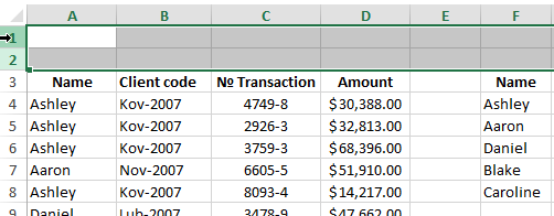
For example, we take the history of mutual settlements with counterparties, as shown in the picture:
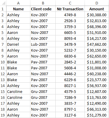
In this table, we need to highlight in color to all transactions for a particular customer. To switch between clients, we will use the drop-down list. Therefore, in the first place, you need to prepare the content for the drop-down list. We need all the customer names from the column A, without repetitions.
Before selecting to the unique values in Excel, we need to prepare the data for the drop-down list:
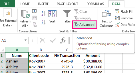
- Select to the first column of the table A1:A19.
- Select to the tool: «DATA»-«Sort and Filter»-«Advanced».
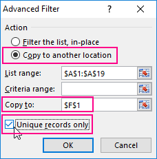
- In the «Advanced Filter» window that appears, you need to turn on «Copy the result to another location», and in the field «Place the result in the range:» to specify $F$1.
- Tick by the check mark to the item «Unique records only» and click OK.
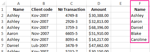
As a result, we got the list of the data with unique values (names without repetitions).
Now we need to slightly modify to our original table. To scroll the first 2 lines and select to the tool: «HOME»-«Cells»-«Insert» or to press the combination of the hot keys CTRL + SHIFT + =.
We have added 2 blank lines. Now we enter in the cell A1 to the value «Client:».
It’s time for creating to the drop-down list, from which we will select customer`s names as the query.
Before you select to the unique values from the list, you need to do the following:
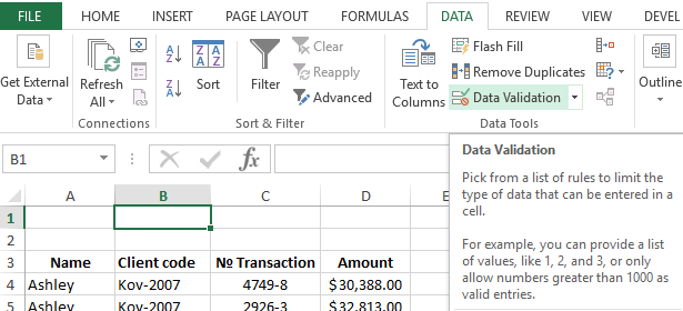
- In the cell B1 you need to select the «DATA»-«Data tool»-«Data Validation».
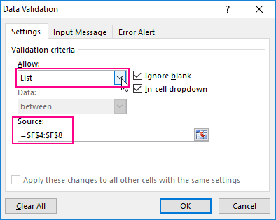
- On the «Settings» tab in the «Validation criteria» section, from the drop-down list «Allow:», you need to select «List» value.
- In the «Source:» entry field, to put =$F$4:$F$8 and click OK.
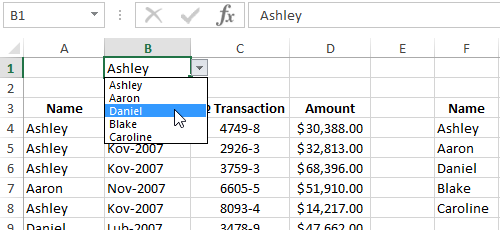
As a result, in the cell B1 we have created the drop-down list of customers` names.
Note. If the data for the drop-down list is in another sheet, then it is better to assign a name for this range and specify it in the «Source:» field. In this case this is not necessary, because all of these data is on the same worksheet.
The selection of the cells from the table by condition in Excel:
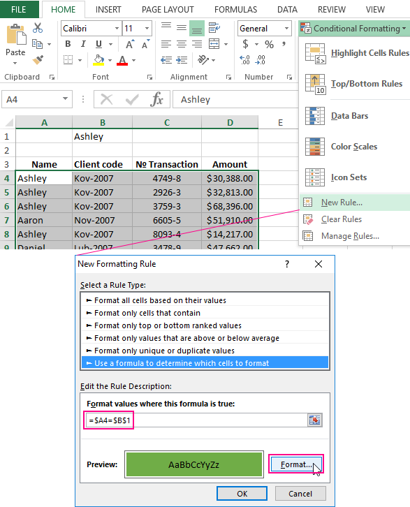
- Highlight the tabular part of the original settlement table A4:D21 and select the tool: «HOME»-«Styles»-«Conditional Formatting»-«New Rule»-«Use the formula to define of the formatted cells».
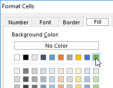
- To select unique values from the column you need to enter the formula: =$A4=$B$1 in the input field and click on the «Format» button to highlight the same cells by color. For example, it will be green color. And to click OK in all are opened windows.
It is done!
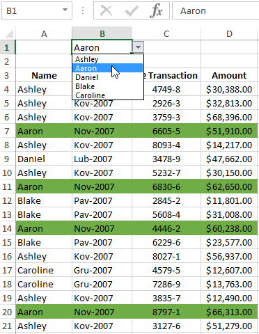
How does work the selection of unique Excel values? When choosing of any value (a name) from the drop-down list B1, all rows that contain this value (name) are highlighted by color in the table. To make sure of this, in the drop-down list B1 you need to choose to a different name. After that, other lines will be automatically highlighted by color. Such table is easy to read and analyze now.
Download example selection from list with conditional formatting.
The principle of automatic highlighting of lines by the query criterion is very simple. Each value in the column A is compared with the value in cell B1. This allows you to find unique values in the Excel table. If the data is the same, then the formula returns to the meaning TRUE and for the whole line is automatically assigned to the new format. In order for the format to be assigned to the entire line, and not just for the cell in column A, we use the mixed reference in the formula =$A4.

Data entry is quicker and more accurate when you use a drop-down list to limit the entries people can make in a cell. When someone selects a cell, the drop-down list’s down-arrow appears, and they can click it and make a selection.
Create a drop-down list
You can make a worksheet more efficient by providing drop-down lists. Someone using your worksheet clicks an arrow, and then clicks an entry in the list.
-
Select the cells that you want to contain the lists.
-
On the ribbon, click DATA > Data Validation.
-
In the dialog, set Allow to List.
-
Click in Source, type the text or numbers (separated by commas, for a comma-delimited list) that you want in your drop-down list, and click OK.
Want more?
Create a drop-down list
Add or remove items from a drop-down list
Remove a drop-down list
Lock cells to protect them
Data entry is quicker and more accurate when you use a drop-down list to limit the entries that people can make in a cell.
When you select a cell, the drop-down list’s down-arrow appears, click it, and make a selection.
Here is how to create drop-down lists: Select the cells that you want to contain the lists.
On the ribbon, click the DATA tab, and click Data Validation.
In the dialog, set Allow to List.
Click in Source.
In this example, we are using a comma-delimited list.
The text or numbers we type in the Source field are separated by commas.
And click OK. The cells now have a drop-down list.
Up next, Drop-down list settings.
Need more help?
Выпадающий список в ячейке листа
Видео
У кого мало времени и нужно быстро ухватить суть — смотрим обучающее видео:
Кому интересны подробности и нюансы всех описанных способов — дальше по тексту.
Способ 1. Примитивный
Один щелчок правой кнопкой мыши по пустой ячейке под столбцом с данными, команда контекстного меню Выбрать из раскрывающегося списка (Choose from drop-down list) или нажать сочетание клавиш ALT+стрелка вниз. Способ не работает, если ячейку и столбец с данными отделяет хотя бы одна пустая строка или вам нужен товар, который еще ни разу не вводился выше:

Способ 2. Стандартный
- Выделите ячейки с данными, которые должны попасть в выпадающий список (например, наименованиями товаров).
- Если у вас Excel 2003 или старше — выберите в меню Вставка — Имя — Присвоить (Insert — Name — Define), если Excel 2007 или новее — откройте вкладку Формулы (Formulas) и воспользуйтесь кнопкой Диспетчер имен (Name Manager), затем Создать. Введите имя (можно любое, но обязательно без пробелов и начать с буквы!) для выделенного диапазона (например Товары). Нажмите ОК.
- Выделите ячейки (можно сразу несколько), в которых хотите получить выпадающий список и выберите в меню (на вкладке) Данные — Проверка (Data — Validation). Из выпадающего списка Тип данных (Allow) выберите вариант Список (List) и введите в строчку Источник (Source) знак равенства и имя диапазона (т.е. =Товары).

Нажмите ОК.
Все! Наслаждайтесь!

Важный нюанс. В качестве источника данных для списка может выступать и динамический именованный диапазон, например прайс-лист. Тогда при дописывании новых товаров к прайсу, они будут автоматически добавляться к выпадающему списку. Еще одним часто используемым трюком для таких списков является создание связанных выпадающих списков (когда содержимое одного списка меняется в зависимости от выбора в другом).
Способ 3. Элемент управления
Этот способ представляет собой вставку на лист нового объекта — элемента управления «поле со списком» с последующей привязкой его к диапазонам на листе. Для этого:
- В Excel 2007/2010 откройте вкладку Разработчик (Developer). В более ранних версиях — панель инструментов Формы (Forms) через меню Вид — Панели инструментов — Формы (View — Toolbars — Forms). Если этой вкладки не видно, то нажмите кнопку Офис — Параметры Excel — флажок Отображать вкладку Разработчик на ленте (Office Button — Excel Options — Show Developer Tab in the Ribbon)
- Найдите значок выпадающего списка среди элементов управления форм (не ActiveX!). Ориентируйтесь по всплывающим подсказкам — Поле со списком:

Щелкните по значку и нарисуйте небольшой горизонтальный прямоугольник — будущий список. - Щелкните по нарисованному списку правой кнопкой мыши и выберите команду Формат объекта (Format control). В появившемся диалоговом окне задайте

- Формировать список по диапазону — выделите ячейки с наименованиями товаров, которые должны попасть в список
- Связь с ячейкой — укажите ячейку куда нужно выводить порядковый номер выбранного пользователем элемента.
- Количество строк списка — сколько строк показывать в выпадающем списке. По умолчанию — 8, но можно больше, чего не позволяет предыдущий способ.
После нажатия на ОК списком можно пользоваться.
Чтобы вместо порядкового номера элемента выводилось его название можно дополнительно использовать функцию ИНДЕКС (INDEX), которая умеет выводить содержимое нужной по счету ячейки из диапазона:

Способ 4. Элемент ActiveX
Этот способ частично напоминает предыдущий. Основное отличие в том, что на лист добавляется не элемент управления, а элемент ActiveX «Поле со списком» из раскрывающегося набора под кнопкой Вставить (Insert) с вкладки Разработчик (Developer):

Механизм добавления тот же — выбираем объект из списка и рисуем его на листе. А вот дальше начинаются серьезные отличия от предыдущего способа.
Во-первых, созданный выпадающий ActiveX список может находится в двух принципиально разных состояниях — режиме отладки, когда можно настраивать его параметры и свойства, двигать его по листу и менять размеры и — режиме ввода, когда единственное, что можно — выбирать из него данные. Переключение между этими режимами происходит с помощью кнопки Режим Конструктора (Design Mode) на вкладке Разработчик (Developer):

Если эта кнопка нажата, то мы можем настраивать параметры выпадающего списка, нажав соседнюю кнопку Свойства (Properties), которая откроет окно со списком всех возможных настроек для выделенного объекта:

Самые нужные и полезные свойства, которые можно и нужно настроить:
- ListFillRange — диапазон ячеек, откуда берутся данные для списка. Выделить мышью диапазон он не даст, надо просто вписать его руками с клавиатуры (например, Лист2!A1:A5)
- LinkedCell — связанная ячейка, куда будет выводиться выбранный из списка элемент
- ListRows — количество отображаемых строк
- Font — шрифт, размер, начертание (курсив, подчеркивание и т.д. кроме цвета)
- ForeColor и BackColor — цвет текста и фона, соответственно
Большим и жирным плюсом этого способа является возможность быстрого перехода к нужному элементу в списке при вводе первых букв с клавиатуры(!), чего нет у всех остальных способов. Приятным моментом, также, является возможность настройки визуального представления (цветов, шрифтов и т.д.)
При использовании этого способа, также возможно указывать в качестве ListFillRange не только одномерные диапазоны. Можно, например задать диапазон из двух столбцов и нескольких строк, указав дополнительно, что выводить нужно два столбца (свойство ColumnCount=2). Тогда можно получить весьма привлекательные результаты, окупающие все потраченные на дополнительные настройки усилия:

Итоговая сравнительная таблица всех способов
| Способ 1. Примитивный | Способ 2. Стандартный | Способ 3. Элемент управления | Способ 4. Элемент ActiveX | |
| Сложность | низкая | средняя | высокая | высокая |
| Возможность настройки шрифта, цвета и т.д. | нет | нет | нет | да |
| Количество отображаемых строк | всегда 8 | всегда 8 | любое | любое |
| Быстрый поиск элемента по первым буквам | нет | нет | нет | да |
| Необходимость использования дополнительной функции ИНДЕКС | нет | нет | да | нет |
| Возможность создания связанных выпадающих списков | нет | да | нет | нет |
Ссылки по теме:
- Выпадающий список с данными из другого файла
- Создание зависимых выпадающих списков
- Автоматическое создание выпадающих списков надстройкой PLEX
- Выбор фото из выпадающего списка
- Автоматическое удаление уже использованных элементов из выпадающего списка
- Выпадающий список с автоматическим добавлением новых элементов
Purpose
Get a value from a list based on position
Return value
The value at the given position.
Usage notes
The CHOOSE function returns a value from a list using a given position or index. The values provided to CHOOSE can be hard-coded constants or cell references. The first argument for the CHOOSE function is index_num. This is a number that refers to subsequent values by index or position. The next arguments, value1, value2, value3, etc. are the values from which to choose from. Choose can handle up to 254 values. However, CHOOSE will not retrieve an item from inside range or array constant provided as a value. For larger sets of data in a table or range, INDEX and MATCH is a better way to retrieve a value based on position.
Examples
The formulas below use CHOOSE to return the 2nd and 3rd values from a list:
CHOOSE(2,"red","blue","green") // returns "blue"
CHOOSE(3,"red","blue","green") // returns "green"
Above, «blue» is the second value, and «green» is the third value. In the example shown in the screenshot, the formula in cell C5 is:
CHOOSE(B5,"red","blue","green") // returns "red"
CHOOSE will not retrieve values from a range or array constant. For example, the formula below will return a #VALUE error:
=CHOOSE(2,A1:A3) // returns #VALUE
This happens because the index number is out of range. In this case, the required syntax is:
=CHOOSE(2,A1,A2,A3)
To retrieve the nth item from a range, use INDEX and MATCH. CHOOSE can be used to provide a variable table to a function like VLOOKUP:
=VLOOKUP(value,CHOOSE(index_num,rng1,rng2),2,0) // variable table
Notes
- If index_num is out of range, CHOOSE will return #VALUE
- Values can also be references. For example, the address A1, or the ranges A1:10 or B2:B15 can be supplied as values.
- CHOOSE will not retrieve values from a range or array constant.
I’m trying to figure out if it is possible to select an Excel item from a list — when that list is in a single cell — using predefined functions, or if I’m going to have to write my own VBA to make it happen.
Something similar to the =CHOOSE() function seems to be what I need, as it works if all of the values are in separate cells:
A B
1alpha =CHOOSE(2,A1,A2,A3,A4,A5)
2beta
3gamma
4delta
5epsilon
The formula above in cell B1 gives me exactly the value I expect: «beta».
But the way my source data are constructed, the values are all in the same cell:
A B
1alpha,beta,gamma,delta,epsilon=CHOOSE(2,A1)
And in this construction, the forumula in B1 results in a #VALUE! error. I do understand why this error occurs — but I’m wondering if there is either:
- Some way to make Excel interpret the comma-separated values in cell A1 as five separate values, or
- Some alternate function I should be using to accomplish this goal.
If Excel can’t handle it, I’ll write my own function — but it seems like such a straightforward need that I assume the program has it built in somewhere.