
IF function
The IF function is one of the most popular functions in Excel, and it allows you to make logical comparisons between a value and what you expect.
So an IF statement can have two results. The first result is if your comparison is True, the second if your comparison is False.
For example, =IF(C2=”Yes”,1,2) says IF(C2 = Yes, then return a 1, otherwise return a 2).

Use the IF function, one of the logical functions, to return one value if a condition is true and another value if it’s false.
IF(logical_test, value_if_true, [value_if_false])
For example:
-
=IF(A2>B2,»Over Budget»,»OK»)
-
=IF(A2=B2,B4-A4,»»)
|
Argument name |
Description |
|---|---|
|
logical_test (required) |
The condition you want to test. |
|
value_if_true (required) |
The value that you want returned if the result of logical_test is TRUE. |
|
value_if_false (optional) |
The value that you want returned if the result of logical_test is FALSE. |
Simple IF examples

-
=IF(C2=”Yes”,1,2)
In the above example, cell D2 says: IF(C2 = Yes, then return a 1, otherwise return a 2)

-
=IF(C2=1,”Yes”,”No”)
In this example, the formula in cell D2 says: IF(C2 = 1, then return Yes, otherwise return No)As you see, the IF function can be used to evaluate both text and values. It can also be used to evaluate errors. You are not limited to only checking if one thing is equal to another and returning a single result, you can also use mathematical operators and perform additional calculations depending on your criteria. You can also nest multiple IF functions together in order to perform multiple comparisons.

-
=IF(C2>B2,”Over Budget”,”Within Budget”)
In the above example, the IF function in D2 is saying IF(C2 Is Greater Than B2, then return “Over Budget”, otherwise return “Within Budget”)

-
=IF(C2>B2,C2-B2,0)
In the above illustration, instead of returning a text result, we are going to return a mathematical calculation. So the formula in E2 is saying IF(Actual is Greater than Budgeted, then Subtract the Budgeted amount from the Actual amount, otherwise return nothing).

-
=IF(E7=”Yes”,F5*0.0825,0)
In this example, the formula in F7 is saying IF(E7 = “Yes”, then calculate the Total Amount in F5 * 8.25%, otherwise no Sales Tax is due so return 0)
Note: If you are going to use text in formulas, you need to wrap the text in quotes (e.g. “Text”). The only exception to that is using TRUE or FALSE, which Excel automatically understands.
Common problems
|
Problem |
What went wrong |
|---|---|
|
0 (zero) in cell |
There was no argument for either value_if_true or value_if_False arguments. To see the right value returned, add argument text to the two arguments, or add TRUE or FALSE to the argument. |
|
#NAME? in cell |
This usually means that the formula is misspelled. |
Need more help?
You can always ask an expert in the Excel Tech Community or get support in the Answers community.

See Also
IF function — nested formulas and avoiding pitfalls
IFS function
Using IF with AND, OR and NOT functions
COUNTIF function
How to avoid broken formulas
Overview of formulas in Excel
Need more help?
In this article we will learn how to color rows based on text criteria we use the “Conditional Formatting” option. This option is available in the “Home Tab” in the “Styles” group in Microsoft Excel.
Conditional Formatting in Excel is used to highlight the data on the basis of some criteria. It would be difficult to see various trends just for examining your Excel worksheet. Conditional Formatting in excel provides a way to visualize data and make worksheets easier to understand.
Excel Conditional Formatting allows you to apply formatting basis on the cell values such as colors, icons and data bars. For this, we will create a rule in excel Conditional Formatting based on cell value
How to write an if statement in excel?
IF function is used for logic_test and returns value on the basis of the result of the logic_test. Excel conditional formatting formula multiple conditions uses Statements like less than or equal to or greater than or equal to the value are used in IF formula
Syntax:
=IF (logical_test, [value_if_true], [value_if_false])
Let’s learn how to do conditional formatting in excel using IF function with the example.
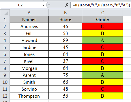
Here is a list of Names and their respective Scores.
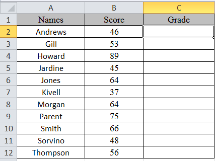
multiple if statements excel functions are used here. So, there are 3 results based on the condition. if then statements in excel is used via excel conditional formatting formula
Write the formula in C2 cell.
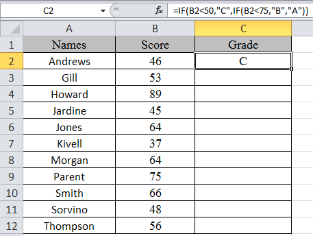
Formula
=IF(B2<50,»C»,IF(B2<75,»B»,»A»))
Explanation:
IF function only returns 2 results, one [value_if_True] and Second [value-if_False]
First IF function checks, if the score is less than 50, would get C grade, The Second IF function tests if the score is less than 75 would get B grade and the rest A grade.
Copy the formula in other cells, select the cells taking the first cell where the formula is already applied, use shortcut key Ctrl + D
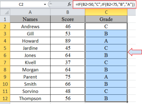
Now we will apply conditional formatting to it.
Select Home >Conditional Formatting > New Rule.
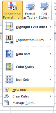
A dialog box appears
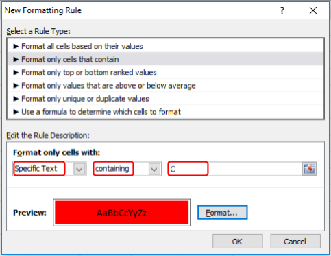
Select Format only cells that contain > Specific text in option list and write C as text to be formatted.
Fill Format with Red colour and click OK.
Now select the colour Yellow and Green for A and B respectively as done above for C.
In this article, we used IF function and Conditional formatting tool to get highlighted grade.
As you can see excel change cell color based on value of another cell using IF function and Conditional formatting tool
Hope you learned how to use conditional formatting in Excel using IF function. Explore more conditional formulas in excel here. You can perform Conditional Formatting in Excel 2016, 2013 and 2010. If you have any unresolved query regarding this article, please do mention below. We will help you.
Related Articles:
How to use the Conditional formatting based on another cell value in Excel
How to use the Conditional Formatting using VBA in Microsoft Excel
How to use the Highlight cells that contain specific text in Excel
How to Sum Multiple Columns with Condition in Excel
Popular Articles:
50 Excel Shortcut to Increase Your Productivity
How to use the VLOOKUP Function in Excel
How to use the COUNTIF function in Excel 2016
How to use the SUMIF Function in Excel
Combine conditional formatting with an IF statement
Syntax
=IF (logical_test, [value_if_true], [value_if_false])
But in conditional formatting, IF/THEN/ELSE syntax cannot be applied in a single rule. Conditional formatting is applied using IF/THEN logical test only. It must return TRUE for conditional formatting to be applied.
For example, if you want to apply conditional formatting using a condition that “If a cell value is greater than a set value, say 100, then format the cell as RED, else format the cell as GREEN”. So, you can see that it requires two rules to perform the conditional formatting, one for greater than 100, and one for less than 100.
You can apply more than one condition by creating more than one rule in conditional formatting. You can also use logical functions like AND and OR to create a rule set and apply conditional formatting in Excel.
Examples using conditional formatting with IF/THEN conditions
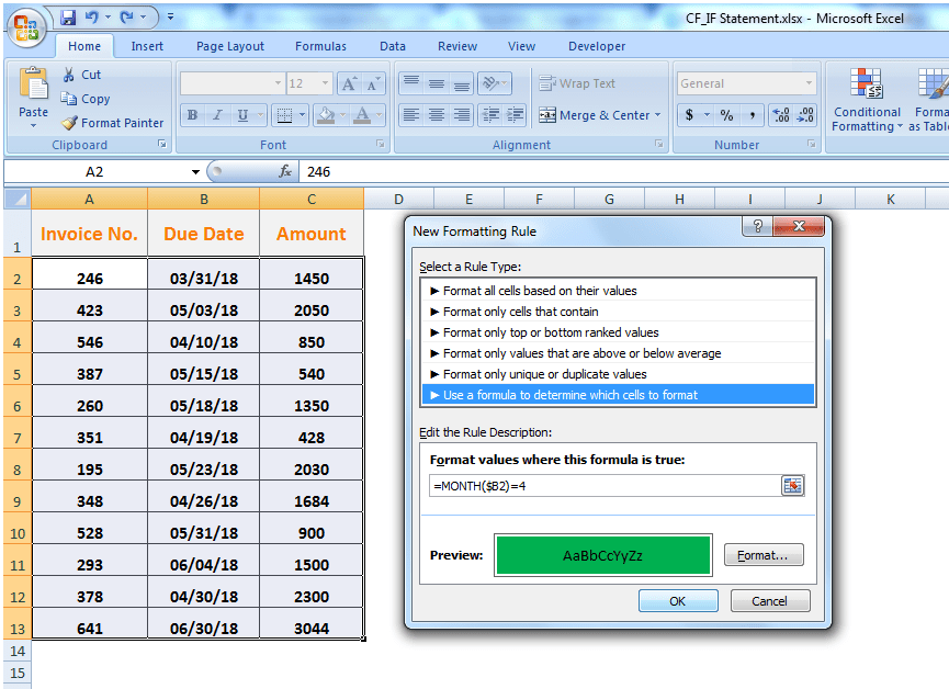
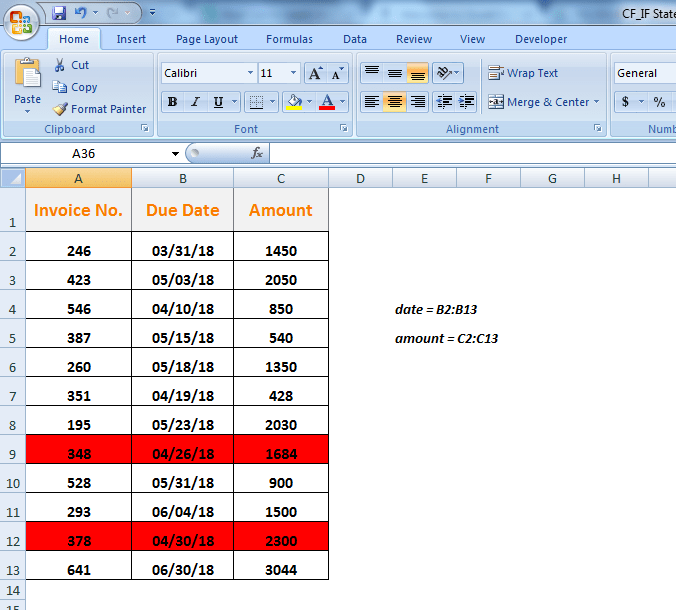
Let’s look at the scenarios to see how to use IF/THEN logical test in conditional formatting to highlight the targeted values. If you want to highlight the invoices in data range of A2:C13 which are due in the month of April, then you need to test the IF/THEN logical condition on date range in column B, if the month is equal to April, by using following custom formula in conditional formatting.=MONTH($B2)=4
First, select the data range A2:C13, then go to:
Conditional Formatting (on the Home tab) > New Rule> Use a formula to determine…> Enter the above formula in Edit Rule Description window> Choose the Format Fill to preview and press OK
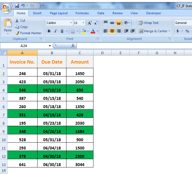
Please note that you have to fix the column by making it absolute using $ sign with it, and keep the row number free or relative to change. Hence, the formula will check each row of the specified column in the selected range, test the IF/THEN logical condition and will return TRUE and FALSE.
This rule will be evaluated in all active cells of locked column B one by one ignoring other cells in columns A and C. When the MONTH function in a cell of column B returns number 4 (April), the rule will return TRUE for all the active cells in that row and conditional formatting will be applied to that entire row as shown below.
Now, if you want to conditionally highlight the two largest amount invoices due in the month of April, then you can achieve this by creating a rule set based on array formula using AND, LARGE and IF statement as per the following syntax.
=AND(criteria,$C2>=LARGE (IF(criteria, values),2)) =AND(MONTH($B2)=criteria,$C2>=LARGE (IF(MONTH(date)=criteria, amount),2)) =AND(MONTH($B2)=4,$C2>=LARGE(IF(MONTH($B$2:$B$13)=4,$C$2:$C$13),2))
By applying this custom formula, you can highlight the two largest amount invoices in the month of April. LARGE with IF function will generate a series of values and compare them with each value in column C. AND function will test the logical conditions in each cell of column B and C both one by one and will return TRUE where both conditions will be met. Have a look below.
Need some additional help with Conditional Formatting or have other questions about Excel? Connect with a live Excel expert here for some 1 on 1 help. Your first session is always free.
Are you still looking for help with the Average function? View our comprehensive round-up of Average function tutorials here.
Maintenance Alert: Saturday, April 15th, 7:00pm-9:00pm CT. During this time, the shopping cart and information requests will be unavailable.
Categories: Conditional Formatting, Excel®
Tags: If/Then Conditional formatting
*Steps in this article will apply to Excel 2007-2016. Images were taken using Excel 2016.
If you are a fan of Excel’s conditional formatting feature, you probably find looking for even more and more ways to highlight useful information in your data. A question that often comes up among these “conditional formatting addicts” is Can I use If/Then formula to format a cell?
The answer is yes and no. Any conditional formatting argument must generate a TRUE result, meaning that at a literal level, your conditional formatting rule is an If/Then statement along the lines of “If this condition is TRUE, THEN format the cell this way”.
What conditional formatting can’t do in a single rule is an IF/THEN/ELSE condition such as “If # is greater than 10 format red, else format green”. Instead, this would require TWO rules, one for “greater than 10” and one for “less than 10”.
Let’s look at a few scenarios to get a sense of how we can create the effect of IF/THEN conditional formatting, even if we can’t use it in the feature itself:
To follow using our examples, download 04-If-Then Conditional Formatting.xlsx
Scenario 1 (Birthdays tab): You want to highlight all employees in your department who have a birthday this month with Red, and all other departments blue.
Solution: Create two rules – one for your department, one for all others
Step 1 – Highlight birthdays in your department
The formula to identify birthdays in the current month will be (see this article for more about using dates in conditional formatting):
=MONTH(C2)=MONTH(TODAY())
To create a formula that generates a TRUE/FALSE statement that highlights birthdays only in one department, you would use the formula:
=AND(MONTH(C2)=MONTH(TODAY()),D2=”Sales”)
This example was created in April, so April birthdays will be highlighted. If you are reproducing the exercise in a different month, you will see different results!
Then, create a second rule for the same range using this formula to highlight birthdays that are not in your department:
=AND(MONTH(C1)=MONTH(TODAY()),D1<>”Sales”)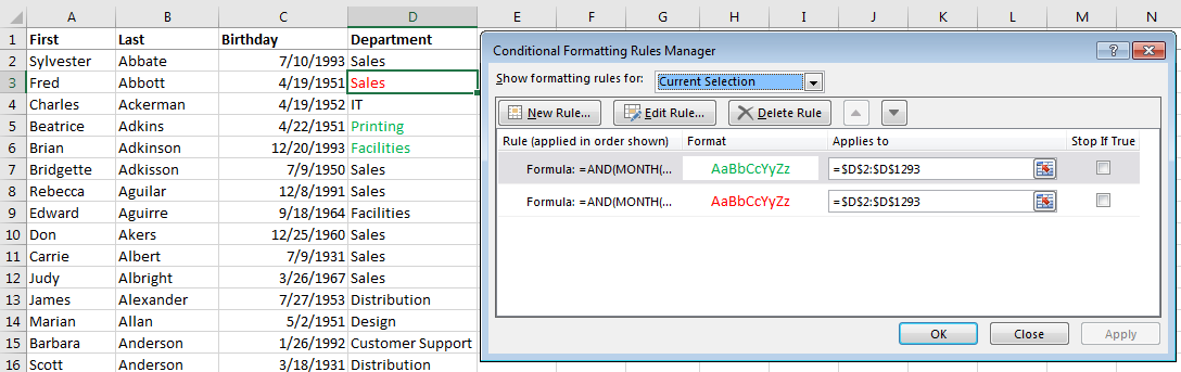
BONUS! In this example, we applied the rule to the department cell to show the relationship to the formula. By changing the Applies to range, however, you can easily highlight a different cell – such as the birthdate – or the entire row. See Get the Most Out of Excel’s Conditional Formatting for more ideas.
Scenario 2 (Retainers tab): You have a table of how many hours your employees have worked for specific clients, and you have a table of how many hours each client has in their retainer budget. You want to highlight the clients who are over their retainer.
Solution 1: Create a helper column using IF/THEN formula to call out whether a client is over their retainer budget. If your worksheet already has the IF/THEN/ELSE logic you need embedded in a cell, Conditional Formatting can act based on those results. You don’t necessarily need to reproduce the logic in the rule itself.
In this example, we already have an IF/THEN formula that returns the result “YES” if our client is over their retainer budget. Our Conditional Formatting rule, then only has to look for the text string “YES” and apply the formatting when true.
Highlight the cell range, Click on Conditional Formatting > Highlight Cell Rules > Text that Contains to create the Rule, then type YES in the Text that Contains dialog box.

Solution 2: Create a formula to calculate retainer budget.
If you don’t have, or don’t want to create, a helper column with an IF/THEN statement, you can use the same method as the first scenario by creating a rule that determines whether a client is over budget. In this example, we applied the rule to the Client cells and the formula would be:
=(F8-G8)<0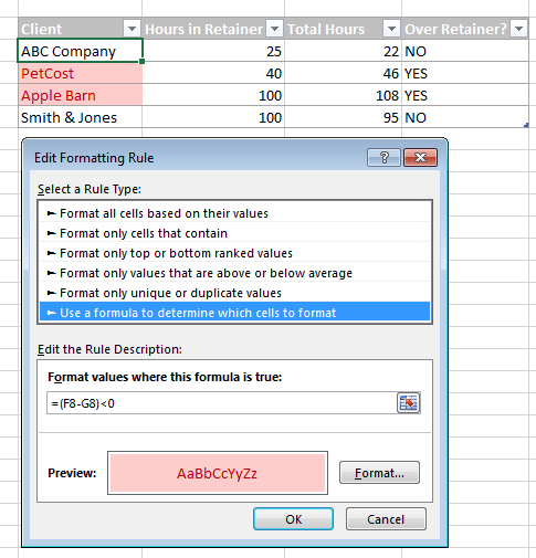
If you are used to creating complex formulas that cover all cases in one cell, it may take a little re-learning to figure out the approach for conditional formatting that works more incrementally. The best hint is to remember that you can apply multiple rules to the same cells – break up your formatting criteria into separate steps, and you’ll most likely be able to get where you need to be!
PRYOR+ 7-DAYS OF FREE TRAINING
Courses in Customer Service, Excel, HR, Leadership,
OSHA and more. No credit card. No commitment. Individuals and teams.
This Excel tutorial explains how to use the Excel IF function with syntax and examples.
Description
The Microsoft Excel IF function returns one value if the condition is TRUE, or another value if the condition is FALSE.
The IF function is a built-in function in Excel that is categorized as a Logical Function. It can be used as a worksheet function (WS) in Excel. As a worksheet function, the IF function can be entered as part of a formula in a cell of a worksheet.
![]() Subscribe
Subscribe
If you want to follow along with this tutorial, download the example spreadsheet.
Download Example
Syntax
The syntax for the IF function in Microsoft Excel is:
IF( condition, value_if_true, [value_if_false] )
Parameters or Arguments
- condition
- The value that you want to test.
- value_if_true
- It is the value that is returned if condition evaluates to TRUE.
- value_if_false
- Optional. It is the value that is returned if condition evaluates to FALSE.
Returns
The IF function returns value_if_true when the condition is TRUE.
The IF function returns value_if_false when the condition is FALSE.
The IF function returns FALSE if the value_if_false parameter is omitted and the condition is FALSE.
Example (as Worksheet Function)
Let’s explore how to use the IF function as a worksheet function in Microsoft Excel.
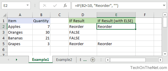
Based on the Excel spreadsheet above, the following IF examples would return:
=IF(B2<10, "Reorder", "")
Result: "Reorder"

=IF(A2="Apples", "Equal", "Not Equal")
Result: "Equal"

=IF(B3>=20, 12, 0)
Result: 12
Combining the IF function with Other Logical Functions
Quite often, you will need to specify more complex conditions when writing your formula in Excel. You can combine the IF function with other logical functions such as AND, OR, etc. Let’s explore this further.
AND function
The IF function can be combined with the AND function to allow you to test for multiple conditions. When using the AND function, all conditions within the AND function must be TRUE for the condition to be met. This comes in very handy in Excel formulas.
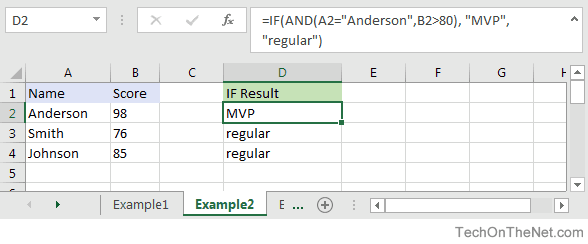
Based on the spreadsheet above, you can combine the IF function with the AND function as follows:
=IF(AND(A2="Anderson",B2>80), "MVP", "regular")
Result: "MVP"

=IF(AND(B2>=80,B2<=100), "Great Score", "Not Bad")
Result: "Great Score"

=IF(AND(B3>=80,B3<=100), "Great Score", "Not Bad")
Result: "Not Bad"

=IF(AND(A2="Anderson",A3="Smith",A4="Johnson"), 100, 50)
Result: 100

=IF(AND(A2="Anderson",A3="Smith",A4="Parker"), 100, 50)
Result: 50
In the examples above, all conditions within the AND function must be TRUE for the condition to be met.
OR function
The IF function can be combined with the OR function to allow you to test for multiple conditions. But in this case, only one or more of the conditions within the OR function needs to be TRUE for the condition to be met.
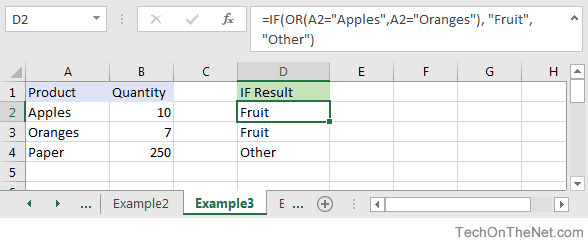
Based on the spreadsheet above, you can combine the IF function with the OR function as follows:
=IF(OR(A2="Apples",A2="Oranges"), "Fruit", "Other")
Result: "Fruit"

=IF(OR(A4="Apples",A4="Oranges"),"Fruit","Other")
Result: "Other"

=IF(OR(A4="Bananas",B4>=100), 999, "N/A")
Result: 999

=IF(OR(A2="Apples",A3="Apples",A4="Apples"), "Fruit", "Other")
Result: "Fruit"
In the examples above, only one of the conditions within the OR function must be TRUE for the condition to be met.
Let’s take a look at one more example that involves ranges of percentages.
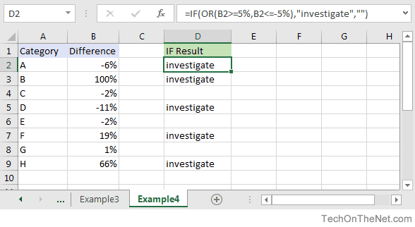
Based on the spreadsheet above, we would have the following formula in cell D2:
=IF(OR(B2>=5%,B2<=-5%),"investigate","")
Result: "investigate"
This IF function would return «investigate» if the value in cell B2 was either below -5% or above 5%. Since -6% is below -5%, it will return «investigate» as the result. We have copied this formula into cells D3 through D9 to show you the results that would be returned.
For example, in cell D3, we would have the following formula:
=IF(OR(B3>=5%,B3<=-5%),"investigate","")
Result: "investigate"
This formula would also return «investigate» but this time, it is because the value in cell B3 is greater than 5%.
Frequently Asked Questions
Question: In Microsoft Excel, I’d like to use the IF function to create the following logic:
if C11>=620, and C10=»F»or»S», and C4<=$1,000,000, and C4<=$500,000, and C7<=85%, and C8<=90%, and C12<=50, and C14<=2, and C15=»OO», and C16=»N», and C19<=48, and C21=»Y», then reference cell A148 on Sheet2. Otherwise, return an empty string.
Answer: The following formula would accomplish what you are trying to do:
=IF(AND(C11>=620, OR(C10="F",C10="S"), C4<=1000000, C4<=500000, C7<=0.85, C8<=0.9, C12<=50, C14<=2, C15="OO", C16="N", C19<=48, C21="Y"), Sheet2!A148, "")
Question: In Microsoft Excel, I’m trying to use the IF function to return 0 if cell A1 is either < 150,000 or > 250,000. Otherwise, it should return A1.
Answer: You can use the OR function to perform an OR condition in the IF function as follows:
=IF(OR(A1<150000,A1>250000),0,A1)
In this example, the formula will return 0 if cell A1 was either less than 150,000 or greater than 250,000. Otherwise, it will return the value in cell A1.
Question: In Microsoft Excel, I’m trying to use the IF function to return 25 if cell A1 > 100 and cell B1 < 200. Otherwise, it should return 0.
Answer: You can use the AND function to perform an AND condition in the IF function as follows:
=IF(AND(A1>100,B1<200),25,0)
In this example, the formula will return 25 if cell A1 is greater than 100 and cell B1 is less than 200. Otherwise, it will return 0.
Question: In Microsoft Excel, I need to write a formula that works this way:
IF (cell A1) is less than 20, then times it by 1,
IF it is greater than or equal to 20 but less than 50, then times it by 2
IF its is greater than or equal to 50 and less than 100, then times it by 3
And if it is great or equal to than 100, then times it by 4
Answer: You can write a nested IF statement to handle this. For example:
=IF(A1<20, A1*1, IF(A1<50, A1*2, IF(A1<100, A1*3, A1*4)))
Question: In Microsoft Excel, I need a formula in cell C5 that does the following:
IF A1+B1 <= 4, return $20
IF A1+B1 > 4 but <= 9, return $35
IF A1+B1 > 9 but <= 14, return $50
IF A1+B1 >= 15, return $75
Answer: In cell C5, you can write a nested IF statement that uses the AND function as follows:
=IF((A1+B1)<=4,20,IF(AND((A1+B1)>4,(A1+B1)<=9),35,IF(AND((A1+B1)>9,(A1+B1)<=14),50,75)))
Question: In Microsoft Excel, I need a formula that does the following:
IF the value in cell A1 is BLANK, then return «BLANK»
IF the value in cell A1 is TEXT, then return «TEXT»
IF the value in cell A1 is NUMERIC, then return «NUM»
Answer: You can write a nested IF statement that uses the ISBLANK function, the ISTEXT function, and the ISNUMBER function as follows:
=IF(ISBLANK(A1)=TRUE,"BLANK",IF(ISTEXT(A1)=TRUE,"TEXT",IF(ISNUMBER(A1)=TRUE,"NUM","")))
Question: In Microsoft Excel, I want to write a formula for the following logic:
IF R1<0.3 AND R2<0.3 AND R3<0.42 THEN «OK» OTHERWISE «NOT OK»
Answer: You can write an IF statement that uses the AND function as follows:
=IF(AND(R1<0.3,R2<0.3,R3<0.42),"OK","NOT OK")
Question: In Microsoft Excel, I need a formula for the following:
IF cell A1= PRADIP then value will be 100
IF cell A1= PRAVIN then value will be 200
IF cell A1= PARTHA then value will be 300
IF cell A1= PAVAN then value will be 400
Answer: You can write an IF statement as follows:
=IF(A1="PRADIP",100,IF(A1="PRAVIN",200,IF(A1="PARTHA",300,IF(A1="PAVAN",400,""))))
Question: In Microsoft Excel, I want to calculate following using an «if» formula:
if A1<100,000 then A1*.1% but minimum 25
and if A1>1,000,000 then A1*.01% but maximum 5000
Answer: You can write a nested IF statement that uses the MAX function and the MIN function as follows:
=IF(A1<100000,MAX(25,A1*0.1%),IF(A1>1000000,MIN(5000,A1*0.01%),""))
Question: In Microsoft Excel, I am trying to create an IF statement that will repopulate the data from a particular cell if the data from the formula in the current cell equals 0. Below is my attempt at creating an IF statement that would populate the data; however, I was unsuccessful.
=IF(IF(ISERROR(M24+((L24-S24)/AA24)),"0",M24+((L24-S24)/AA24)))=0,L24)
The initial part of the formula calculates the EAC (Estimate At completion = AC+(BAC-EV)/CPI); however if the current EV (Earned Value) is zero, the EAC will equal zero. IF the outcome is zero, I would like the BAC (Budget At Completion), currently recorded in another cell (L24), to be repopulated in the current cell as the EAC.
Answer: You can write an IF statement that uses the OR function and the ISERROR function as follows:
=IF(OR(S24=0,ISERROR(M24+((L24-S24)/AA24))),L24,M24+((L24-S24)/AA24))
Question: I have been looking at your Excel IF, AND and OR sections and found this very helpful, however I cannot find the right way to write a formula to express if C2 is either 1,2,3,4,5,6,7,8,9 and F2 is F and F3 is either D,F,B,L,R,C then give a value of 1 if not then 0. I have tried many formulas but just can’t get it right, can you help please?
Answer: You can write an IF statement that uses the AND function and the OR function as follows:
=IF(AND(C2>=1,C2<=9, F2="F",OR(F3="D",F3="F",F3="B",F3="L",F3="R",F3="C")),1,0)
Question:In Excel, I have a roadspeed of a car in m/s in cell A1 and a drop down menu of different units in C1 (which unclude mph and kmh). I have used the following IF function in B1 to convert the number to the unit selected from the dropdown box:
=IF(C1="mph","=A1*2.23693629",IF(C1="kmh","A1*3.6"))
However say if kmh was selected B1 literally just shows A1*3.6 and does not actually calculate it. Is there away to get it to calculate it instead of just showing the text message?
Answer: You are very close with your formula. Because you are performing mathematical operations (such as A1*2.23693629 and A1*3.6), you do not need to surround the mathematical formulas in quotes. Quotes are necessary when you are evaluating strings, not performing math.
Try the following:
=IF(C1="mph",A1*2.23693629,IF(C1="kmh",A1*3.6))
Question:For an IF statement in Excel, I want to combine text and a value.
For example, I want to put an equation for work hours and pay. IF I am paid more than I should be, I want it to read how many hours I owe my boss. But if I work more than I am paid for, I want it to read what my boss owes me (hours*Pay per Hour).
I tried the following:
=IF(A2<0,"I owe boss" abs(A2) "Hours","Boss owes me" abs(A2)*15 "dollars")
Is it possible or do I have to do it in 2 separate cells? (one for text and one for the value)
Answer: There are two ways that you can concatenate text and values. The first is by using the & character to concatenate:
=IF(A2<0,"I owe boss " & ABS(A2) & " Hours","Boss owes me " & ABS(A2)*15 & " dollars")
Or the second method is to use the CONCATENATE function:
=IF(A2<0,CONCATENATE("I owe boss ", ABS(A2)," Hours"), CONCATENATE("Boss owes me ", ABS(A2)*15, " dollars"))
Question:I have Excel 2000. IF cell A2 is greater than or equal to 0 then add to C1. IF cell B2 is greater than or equal to 0 then subtract from C1. IF both A2 and B2 are blank then equals C1. Can you help me with the IF function on this one?
Answer: You can write a nested IF statement that uses the AND function and the ISBLANK function as follows:
=IF(AND(ISBLANK(A2)=FALSE,A2>=0),C1+A2, IF(AND(ISBLANK(B2)=FALSE,B2>=0),C1-B2, IF(AND(ISBLANK(A2)=TRUE, ISBLANK(B2)=TRUE),C1,"")))
Question:How would I write this equation in Excel? IF D12<=0 then D12*L12, IF D12 is > 0 but <=600 then D12*F12, IF D12 is >600 then ((600*F12)+((D12-600)*E12))
Answer: You can write a nested IF statement as follows:
=IF(D12<=0,D12*L12,IF(D12>600,((600*F12)+((D12-600)*E12)),D12*F12))
Question:In Excel, I have this formula currently:
=IF(OR(A1>=40, B1>=40, C1>=40), "20", (A1+B1+C1)-20)
If one of my salesman does sale for $40-$49, then his commission is $20; however if his/her sale is less (for example $35) then the commission is that amount minus $20 ($35-$20=$15). I have 3 columns that are needed based on the type of sale. Only one column per row will be needed. The problem is that, when left blank, the total in the formula cell is -20. I need help setting up this formula so that when the 3 columns are left blank, the cell with the formula is left blank as well.
Answer: Using the AND function and the ISBLANK function, you can write your IF statement as follows:
=IF(AND(ISBLANK(A1),ISBLANK(B1),ISBLANK(C1)),"",IF(OR(A1>40, B1>40, C1>40), "20", (A1+B1+C1)-20))
In this formula, we are using the ISBLANK function to check if all 3 cells A1, B1, and C1 are blank, and if they are return a blank value («»). Then the rest is the formula that you originally wrote.
Question:In Excel, I need to create a simple booking and and out system, that shows a date out and a date back
«A1» = allows person to input date booked out
«A2» =allows person to input date booked back in
«A3″= shows status of product, eg, booked out, overdue return etc.
I can automate A3 with the following IF function:
=IF(ISBLANK(A2),"booked out","returned")
But what I cant get to work is if the product is out for 10 days or more, I would like the cell to say «send email»
Can you assist?
Answer: Using the TODAY function and adding an additional IF function, you can write your formula as follows:
=IF(ISBLANK(A2),IF(TODAY()-A1>10,"send email","booked out"),"returned")
Question:Using Microsoft Excel, I need a formula in cell U2 that does the following:
IF the date in E2<=12/31/2010, return T2*0.75
IF the date in E2>12/31/2010 but <=12/31/2011, return T2*0.5
IF the date in E2>12/31/2011, return T2*0
I tried using the following formula, but it gives me «#VALUE!»
=IF(E2<=DATE(2010,12,31),T2*0.75), IF(AND(E2>DATE(2010,12,31),E2<=DATE(2011,12,31)),T2*0.5,T2*0)
Can someone please help? Thanks.
Answer: You were very close…you just need to adjust your parentheses as follows:
=IF(E2<=DATE(2010,12,31),T2*0.75, IF(AND(E2>DATE(2010,12,31),E2<=DATE(2011,12,31)),T2*0.5,T2*0))
Question:In Excel, I would like to add 60 days if grade is ‘A’, 45 days if grade is ‘B’ and 30 days if grade is ‘C’. It would roughly look something like this, but I’m struggling with commas, brackets, etc.
(IF C5=A)=DATE(YEAR(B5)+0,MONTH(B5)+0,DAY(B5)+60),
(IF C5=B)=DATE(YEAR(B5)+0,MONTH(B5)+0,DAY(B5)+45),
(IF C5=C)=DATE(YEAR(B5)+0,MONTH(B5)+0,DAY(B5)+30)
Answer:You should be able to achieve your date calculations with the following formula:
=IF(C5="A",B5+60,IF(C5="B",B5+45,IF(C5="C",B5+30)))
Question:In Excel, I am trying to write a function and can’t seem to figure it out. Could you help?
IF D3 is < 31, then 1.51
IF D3 is between 31-90, then 3.40
IF D3 is between 91-120, then 4.60
IF D3 is > 121, then 5.44
Answer:You can write your formula as follows:
=IF(D3>121,5.44,IF(D3>=91,4.6,IF(D3>=31,3.4,1.51)))
Question:I would like ask a question regarding the IF statement. How would I write in Excel this problem?
I have to check if cell A1 is empty and if not, check if the value is less than equal to 5. Then multiply the amount entered in cell A1 by .60. The answer will be displayed on Cell A2.
Answer:You can write your formula in cell A2 using the IF function and ISBLANK function as follows:
=IF(AND(ISBLANK(A1)=FALSE,A1<=5),A1*0.6,"")
Question:In Excel, I’m trying to nest an OR command and I can’t find the proper way to write it. I want the spreadsheet to do the following:
If D6 equals «HOUSE» and C6 equals either «MOUSE» or «CAT», I want to return the value in cell B6. Otherwise, the formula should return the value «BLANK».
I tried the following:
=IF((D6="HOUSE")*(C6="MOUSE")*OR(C6="CAT"));B6;"BLANK")
If I only ask for HOUSE and MOUSE or HOUSE and CAT, it works, but as soon as I ask for MOUSE OR CAT, it doesn’t work.
Answer:You can write your formula using the AND function and OR function as follows:
=IF(AND(D6="HOUSE",OR(C6="MOUSE",C6="CAT")),B6,"BLANK")
This will return the value in B6 if D6 equals «HOUSE» and C6 equals either «MOUSE» or «CAT». If those conditions are not met, the formula will return the text value of «BLANK».
Question:In Microsoft Excel, I’m trying to write the following formula:
If cell A1 equals «jaipur», «udaipur» or «jodhpur», then cell A2 should display «rajasthan»
If cell A1 equals «bangalore», «mysore» or «belgum», then cell A2 should display «karnataka»
Please help.
Answer:You can write your formula using the OR function as follows:
=IF(OR(A1="jaipur",A1="udaipur",A1="jodhpur"),"rajasthan", IF(OR(A1="bangalore",A1="mysore",A1="belgum"),"karnataka"))
This will return «rajasthan» if A1 equals either «jaipur», «udaipur» or «jodhpur» and it will return «karnataka» if A1 equals either «bangalore», «mysore» or «belgum».
Question:In Microsoft Excel I’m trying to achieve the following with IF function:
If a value in any cell in column F is «food» then add the value of its corresponding cell in column G (eg a corresponding cell for F3 is G3). The IF function is performed in another cell altogether. I can do it for a single pair of cells but I don’t know how to do it for an entire column. Could you help?
At the moment, I’ve got this:
=IF(F3="food"; G3; 0)
Answer:This formula can be created using the SUMIF formula instead of using the IF function:
=SUMIF(F1:F10,"=food",G1:G10)
This will evaluate the first 10 rows of data in your spreadsheet. You may need to adjust the ranges accordingly.
I notice that you separate your parameters with semi-colons, so you might need to replace the commas in the formula above with semi-colons.
Question:I’m looking for an Exel formula that says:
If F3 is «H» and E3 is «H», return 1
If F3 is «A» and E3 is «A», return 2
If F3 is «d» and E3 is «d», return 3
Appreciate if you can help.
Answer:This Excel formula can be created using the AND formula in combination with the IF function:
=IF(AND(F3="H",E3="H"),1,IF(AND(F3="A",E3="A"),2,IF(AND(F3="d",E3="d"),3,"")))
We’ve defaulted the formula to return a blank if none of the conditions above are met.
Question:I am trying to get Excel to check different boxes and check if there is text/numbers listed in the cells and then spit out «Complete» if all 5 Boxes have text/Numbers or «Not Complete» if one or more is empty. This is what I have so far and it doesn’t work.
=IF(OR(ISBLANK(J2),ISBLANK(M2),ISBLANK(R2),ISBLANK (AA2),ISBLANK (AB2)),"Not Complete","")
Answer:First, you are correct in using the ISBLANK function, however, you have a space between ISBLANK and (AA2), as well as ISBLANK and (AB2). This might seem insignificant, but Excel can be very picky and will return a #NAME? error. So first you need to eliminate those spaces.
Next, you need to change the ELSE condition of your IF function to return «Complete».
You should be able to modify your formula as follows:
=IF(OR(ISBLANK(J2),ISBLANK(M2),ISBLANK(R2),ISBLANK(AA2),ISBLANK(AB2)), "Not Complete", "Complete")
Now if any of the cell J2, M2, R2, AA2, or AB2 are blank, the formula will return «Not Complete». If all 5 cells have a value, the formula will return «Complete».
Question:I’m very new to the Excel world, and I’m trying to figure out how to set up the proper formula for an If/then cell.
What I’m trying for is:
If B2’s value is 1 to 5, then multiply E2 by .77
If B2’s value is 6 to 10, then multiply E2 by .735
If B2’s value is 11 to 19, then multiply E2 by .7
If B2’s value is 20 to 29, then multiply E2 by .675
If B2’s value is 30 to 39, then multiply E2 by .65
I’ve tried a few different things thinking I was on the right track based on the IF, and AND function tutorials here, but I can’t seem to get it right.
Answer:To write your IF formula, you need to nest multiple IF functions together in combination with the AND function.
The following formula should work for what you are trying to do:
=IF(AND(B2>=1, B2<=5), E2*0.77, IF(AND(B2>=6, B2<=10), E2*0.735, IF(AND(B2>=11, B2<=19), E2*0.7, IF(AND(B2>=20, B2<=29), E2*0.675, IF(AND(B2>=30, B2<=39), E2*0.65,"")))))
As one final component of your formula, you need to decide what to do when none of the conditions are met. In this example, we have returned «» when the value in B2 does not meet any of the IF conditions above.
Question:Here is the Excel formula that has me between a rock and a hard place.
If E45 <= 50, return 44.55
If E45 > 50 and E45 < 100, return 42
If E45 >=200, return 39.6
Again thank you very much.
Answer:You should be able to write this Excel formula using a combination of the IF function and the AND function.
The following formula should work:
=IF(E45<=50, 44.55, IF(AND(E45>50, E45<100), 42, IF(E45>=200, 39.6, "")))
Please note that if none of the conditions are met, the Excel formula will return «» as the result.
Question:I have a nesting OR function problem:
My nonworking formula is:
=IF(C9=1,K9/J7,IF(C9=2,K9/J7,IF(C9=3,K9/L7,IF(C9=4,0,K9/N7))))
In Cell C9, I can have an input of 1, 2, 3, 4 or 0. The problem is on how to write the «or» condition when a «4 or 0» exists in Column C. If the «4 or 0» conditions exists in Column C I want Column K divided by Column N and the answer to be placed in Column M and associated row
Answer:You should be able to use the OR function within your IF function to test for C9=4 OR C9=0 as follows:
=IF(C9=1,K9/J7,IF(C9=2,K9/J7,IF(C9=3,K9/L7,IF(OR(C9=4,C9=0),K9/N7))))
This formula will return K9/N7 if cell C9 is either 4 or 0.
Question:In Excel, I am trying to create a formula that will show the following:
If column B = Ross and column C = 8 then in cell AB of that row I want it to show 2013, If column B = Block and column C = 9 then in cell AB of that row I want it to show 2012.
Answer:You can create your Excel formula using nested IF functions with the AND function.
=IF(AND(B1="Ross",C1=8),2013,IF(AND(B1="Block",C1=9),2012,""))
This formula will return 2013 as a numeric value if B1 is «Ross» and C1 is 8, or 2012 as a numeric value if B1 is «Block» and C1 is 9. Otherwise, it will return blank, as denoted by «».
Question:In Excel, I really have a problem looking for the right formula to express the following:
If B1=0, C1 is equal to A1/2
If B1=1, C1 is equal to A1/2 times 20%
If D1=1, C1 is equal to A1/2-5
I’ve been trying to look for any same expressions in your site. Please help me fix this.
Answer:In cell C1, you can use the following Excel formula with 3 nested IF functions:
=IF(B1=0,A1/2, IF(B1=1,(A1/2)*0.2, IF(D1=1,(A1/2)-5,"")))
Please note that if none of the conditions are met, the Excel formula will return «» as the result.
Question:In Excel, I need the answer for an IF THEN statement which compares column A and B and has an «OR condition» for column C. My problem is I want column D to return yes if A1 and B1 are >=3 or C1 is >=1.
Answer:You can create your Excel IF formula as follows:
=IF(OR(AND(A1>=3,B1>=3),C1>=1),"yes","")
Please note that if none of the conditions are met, the Excel formula will return «» as the result.
Question:In Excel, what have I done wrong with this formula?
=IF(OR(ISBLANK(C9),ISBLANK(B9)),"",IF(ISBLANK(C9),D9-TODAY(), "Reactivated"))
I want to make an event that if B9 and C9 is empty, the value would be empty. If only C9 is empty, then the output would be the remaining days left between the two dates, and if the two cells are not empty, the output should be the string ‘Reactivated’.
The problem with this code is that IF(ISBLANK(C9),D9-TODAY() is not working.
Answer:First of all, you might want to replace your OR function with the AND function, so that your Excel IF formula looks like this:
=IF(AND(ISBLANK(C9),ISBLANK(B9)),"",IF(ISBLANK(C9),D9-TODAY(),"Reactivated"))
Next, make sure that you don’t have any abnormal formatting in the cell that contains the results. To be safe, right click on the cell that contains the formula and choose Format Cells from the popup menu. When the Format Cells window appears, select the Number tab. Choose General as the format and click on the OK button.
Question:I was wondering if you could tell me what I am doing wrong.
Here are the instructions:
A customer is eligible for a discount if the customer’s 2016 sales greater than or equal to 100000 OR if the customers First Order was placed in 2016.
If the customer qualifies for a discount, return a value of Y
If the customer does not qualify for a discount, return a value of N.
Here is the formula I’ve entered:
=IF(OR([2014 Sales]=0,[2015 Sales]=0,[2016 Sales]>=100000),"Y","N")
I only have 2 cells wrong. Can you help me please? I am very lost and confused.
Answer:You are very close with your IF formula, however, it looks like you need to add the AND function to your formula as follows:
=IF(OR([2016 Sales]>=100000,AND([2014 Sales]=0,[2015 Sales]=0),C8>=100000),"Y","N")
This formula should return Y if 2016 sales are greater than or equal to 100000, or if both 2014 sales and 2015 sales are 0. Otherwise, the formula will return N. You will also notice that we switched the order of your conditions in the formula so that it is easier to understand the formula based on your instructions above.
Question:Could you please help me? I need to use «OR» on my formula but I can’t get it to work. This is what I’ve tried:
=IF(C6>=0<=150,150000,IF(C6>=151<=160,158400))
Here is what I need the formula to do:
IF C6 IS >=0 OR <=150 THEN ASSIGN $150000
IF C6 IS >=151 OR <=160 THEN ASSIGN $158400
Answer:You should be able to use the AND function within your IF function as follows:
=IF(AND(ISBLANK(C6)=FALSE,C6>=0,C6<=150),150000,IF(AND(C6>=151,C6<=160),158400,""))
Notice that we first use the ISBLANK function to test C6 to make sure that it is not blank. This is because if C6 if blank, it will evalulate to greater than 0 and thus return 150000. To avoid this, we include ISBLANK(C6)=FALSE as one of the conditions in addition to C6>=0 and C6<=150. That way, you won’t return any false results if C6 is blank.
Question:I am having a problem with a formula, I want it to be IF E5=N then do the first formula, else do the second formula. Excel recognizes the =IF(logical_test,value_if_TRUE,value_if_FALSE) but doesn’t like the formula below:
=IF(e5="N",((AND(AH5-AG5<456, AH5-S5<822)), "Compliant", "not Compliant"),((AH5-S5<822), "Compliant", "not Compliant"))
Any help would be greatly appreciated.
Answer:To have the first formula executed when E5=N and then second formula executed when E5<>N, you will need to nest 2 additional IF functions within the main IF function as follows:
=IF(E5="N", IF((AND(AH5-AG5<456, AH5-S5<822)), "Compliant", "not Compliant"), IF((AH5-S5<822), "Compliant", "not Compliant"))
If E5=»N», the first nested IF function will be executed:
IF((AND(AH5-AG5<456, AH5-S5<822)), "Compliant", "not Compliant")
Otherwise,the second nested IF function will be executed:
IF((AH5-S5<822), "Compliant", "not Compliant"))
Question:I need to write a formula based on the following logic:
There is a maximum discount allowed of £1000 if the capital sum is less that £43000 and a lower discount of £500 if the capital sum is above £43000. So the formula should return either £500 or £1000 in the cell but the £43000 is made up of two numbers, say for e.g. £42750+350 and if the second number is less than the allowed discount, the actual lower value is returned — in this case the £500 or £1000 becomes £350. Or as another e.g. £42000+750 returns £750.
So on my spreadsheet, in this second e.g. I would have A1= £42000, A2=750, A3=A1+A2, A4=the formula with the changing discount, in this case £750.
How can I write this formula?
Answer:In cell A4, you can calculate the correct discount using the IF function and the MIN function as follows:
=IF(A3<43000, MIN(A2,1000), MIN(A2,500))
If A3 is less than 43000, the formula will return the lower value of A2 and 1000. Otherwise, it will return the lower value of A2 and 500.
Question: I have a list of sizes in column A with sizes 100, 200, 300, 400, 500, 600. Then I have another column B, with sizes of my products, and it is random, for example, 318, 445, 527. What I’m trying to create is for a value of 318 in column B, I need to return 400 for that product. If the value in column B is 445, then I should return 500 and so on, as long sizes in column A must be BIGGER to the NEAREST size to column B.
Any idea how to create this function?
Answer:If your sizes are in increments of 100, you can create this function by taking the value in column B, dividing by 100, rounding up to the nearest integer, and then multiplying by 100.
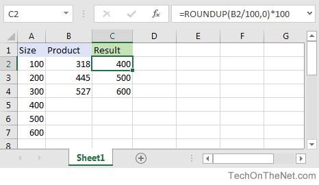
For example in cell C2, you can use the IF function and the ROUNDUP function as follows:
=ROUNDUP(B2/100,0)*100
This will return the correct value of 400 for a value of 318 in cell B2. Just copy this formula to cell C3, C4 and so on.