Excel cell format change

When you fill out Excel worksheets with data, no one will succeed at once, everything is beautiful and correctly filled at the first attempt.

In the process of working with the program, you always need something: modify, edit, delete, copy or move. If the entered incorrect values in a cell, naturally, we want to correct or delete ones. But even such simple task can sometimes create difficulties.



How to set the cell format in Excel?

The contents of each Excel cell consist of three elements:

1. The meaning: text, numbers, dates and times, logical content, functions and formulas.
2. The formats: the type and color of the borders, the type and color of the fill, the way the values are displayed.
3. Comments.

All these three elements are completely independent of each other. You can specify the format of the cell and do not write anything to it, or add a note in an empty and not formatted cell.



How to change the format of cells in Excel?

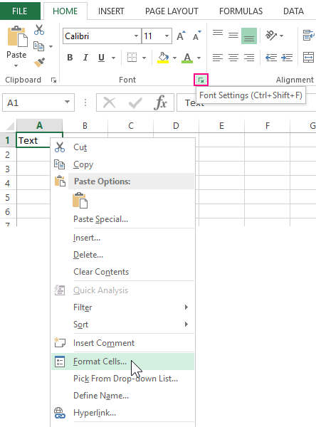
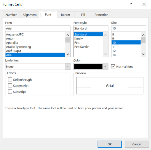
To change the format of the cells, you should call the corresponding dialog box with the CTRL + 1 (or CTRL + SHIFT + F) key or from the context menu after you right-click the «Cell Format» option.

There are 6 tabs in this dialog box:

1. A number. Here you specify the way the numeric values are displayed.
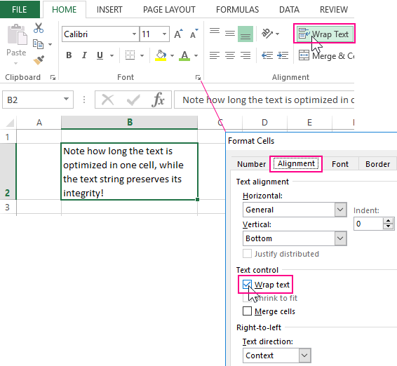
2. The alignment. On this tab you can control the position of the text. And the text can be displayed vertically or diagonally from any angle. Also pay attention to the «Display» section. Very often, the function «Wrap Text» is used.



3. Font. The specify the style design of fonts, the size and color of the text, plus the modes of modifications.
4. The border. Here you define the styles and colors of the borders. The design of all tables is better done right here.
5. The fill. The name of the bookmark speaks for itself. Available for formatting colors, patterns and methods of filling (for example, a gradient with a different direction of strokes).
6. The protection. Here, the cell protection settings are set, that are activated only after the protection of the whole sheet.

If you did not get the desired result on the first attempt, call this dialog again to fix the cell format in Excel.

What formatting is applicable to cells in Excel?

Each cell always has some format. If there were no changes, then this is the «General» format. It is also a standard Excel format, in which:

• the numbers are aligned on the right side;
• the text is aligned on the left side;
• the font Calibri with the height of 11 points;
• the cell has no borders and background fill.

The Format Removal – is the changing to the standard «General» format (without borders and fills).

It is worth noting that the format of cells, unlike values, can not be deleted with the DELETE key.

To delete the format of cells, select ones and use the «Clear Formats» tool, which is located on the «HOME» tab in the «Editing» section.

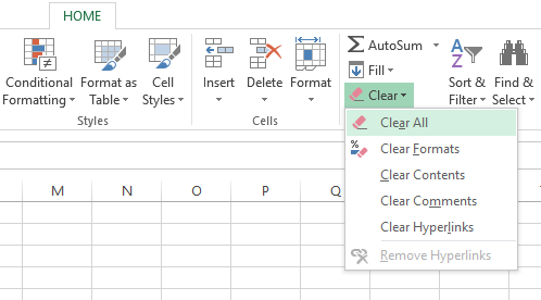
If you want to clear not only the format, but also the values, then select the «Clear All» option from the drop-down list of the tool (eraser).

As you can see, the eraser tool is functionally flexible and allows us to make a choice of what to delete in the cells:

• the content (same as the DELETE key);
• the formats;
• notes;
• the hyperlinks.

The option «Clear all» combines all these functions.

The deleting notes

Note, as well as formats, are not deleted from the cell by pressing the DELETE key. You can delete notes in two ways:

1. The eraser tool: the option «Clear notes».
2. Click on the cell with the note with the right mouse button, and from the appeared context menu select the option «Delete note».

The notation. The second way is more convenient. If you delete several notes at the same time, you must first select all of its cells.

Does this sound familiar? You work on an Excel sheet and are almost done with it. Now, you just want to “brush it up” a bit. But: It seems that the formatting takes even longer than working on the calculations. In this article we look at techniques to apply a format with as few clicks as possible. Let’s start saving time now!

Method 1: How to format cells manually

Potential time saving:

Well, probably you are not here for learning it the long, inconvenient way. But anyway, I quickly summarize how to apply a format the “traditional” way in Excel.

Actually, there are several way to change font, number formatting, colors, borders. The first one would be via the ribbon:

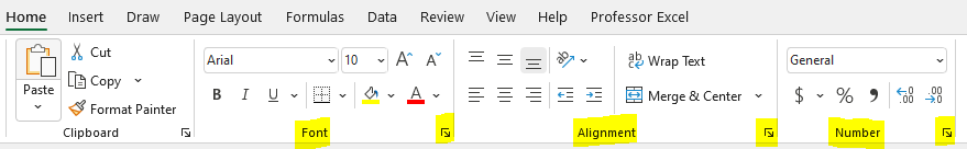
On the Home ribbon, you can find the quick settings of font style, colors, borders and so in the “Font” group. Next to it, you can see further settings in the “Alignment” group and the “Number” group. Everything, no need to elaborate that in detail.

One comment: the small arrows in the corners (also highlighted yellow), lead to the Format cells window. It contains more detailed formatting options. Alternatively, you can just press Ctrl + 1 on the keyboard to open that window.

Method 2: Shortcut formatting with the format painter

Potential time saving:

Once you have perfectly formatted a cell (for example with the method 1 above). With the Format Painter, you can easily transfer this formatting to a different cell.

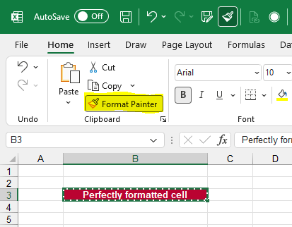
1. Select the original cells.
2. Click on the Format Painter on the Home ribbon.
3. Click on the unformatted cell to apply the format.

You want to apply this cell layout to multiple cells? Double click on the format painter and the you can click on all desired cells until you press Esc or click on the Format Painter button again.

Also: It works for whole ranges of cells. You can just select multiple cells and press on the Format Painter button.

Recommendation: This could be a great button for the Quick Access Toolbar. I have added it to my Quick Access Toolbar – in all Office programs at the same position. Now, when I press the Alt button and afterwards 4 (because it is in the forth position in my Quick Access Toolbar), I can quickly use it without the mouse.

Method 3: Apply cell styles to save a lot of time

Potential time saving:

Now, we get increasingly faster with formatting. Our next advice is to use the built-in cell styles.

Cell styles are a great way to apply layout settings to single cells are cell ranges. And later, you can easily change the format within the cell style definition.

Here is, how it works:

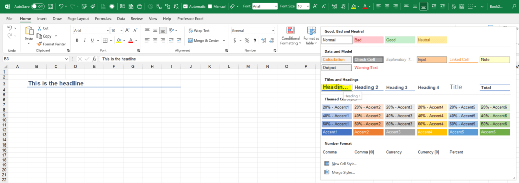
1. Select one or multiple cells.
2. Click on your desired cell style. It’s located on the Home ribbon in the Styles section.

Changing a cell style is quite simple, but requires some clicks through the menues.

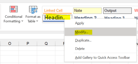
1. Right-click on the style you want to change.
2. Then, click on Modify.
3. Now, you can click on “Format” to change the settings in detail.

The changes will be applied to all cells that use this particular style.

Disadvantages:

• When you copy worksheets several times from different files, cell styles might accumulated. I have noticed that especially for some Excel exports, for example from SAP.
• If you change a cell style, it only applies to the current Excel workbook. When you create a new Excel file, you have to do the same changes again.

Method 4: Use Office themes

Potential time saving:

This method works best when you already have a “clean” formatting in your Excel file. For example, if you have consequently used the cell styles in method 3 above.

But nonetheless, it’s often a worth a try: Create your own Office theme. This can save a lot of time when it comes to colors and fonts. The advantage: You can save a theme and use it throughout the Office suite. That way, you can transfer your corporate colors to all your documents.

How it works? Quit simple:

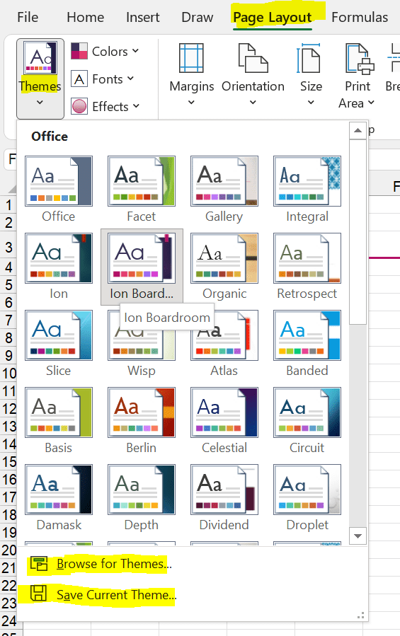
1. Go to the Page Layout ribbon.
2. Click on the theme that is already close to your desired layout.
3. Modify colors and fonts with the buttons right next to the Themes button.
4. Click on “Save Current Theme”.

Next time you want to use this theme, just click on “Browse for theme” and select it on your hard drive.

Method 5: Use Professor Excel Tools to use your individual formatting – with just one click

Potential time saving:

This is probably the feature I use most often of the Excel add-in “Professor Excel Tools“. It’s fair to say that I have saved days, maybe even weeks of work just with these two buttons.

1. Just select the cells to format.
2. Click on either the headline or content / body button.

As you can see, it’s very fast, right?

The good thing about this method: You just define it once – and you can apply the formatting to any workbook.

Defining your favorite formats is also very easy:

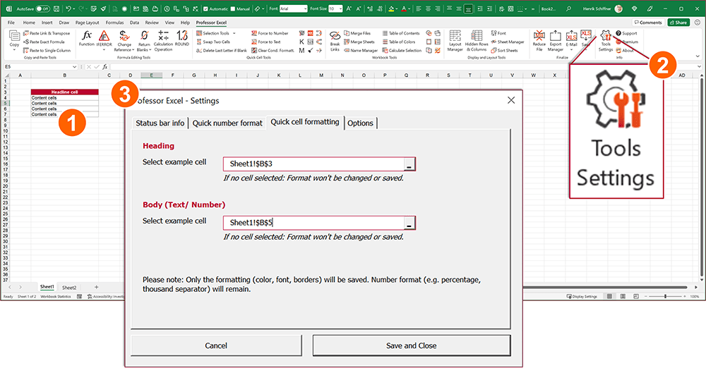
1. Apply your favorite heading or content / body layout to a cell.
2. Go to the Tools Settings (on the right side of the Professor Excel ribbon).
3. On the “Quick cell formatting” tab, select your pre-formatted example cells for heading and body. Click on Save and Close to save the formatting.

---

This function is included in our Excel Add-In ‘Professor Excel Tools’

(No sign-up, download starts directly)

---

Image by garageband from Pixabay