
Select cell contents in Excel
In Excel, you can select cell contents of one or more cells, rows and columns.

Note: If a worksheet has been protected, you might not be able to select cells or their contents on a worksheet.
Select one or more cells
-
Click on a cell to select it. Or use the keyboard to navigate to it and select it.
-
To select a range, select a cell, then with the left mouse button pressed, drag over the other cells.
Or use the Shift + arrow keys to select the range.
-
To select non-adjacent cells and cell ranges, hold Ctrl and select the cells.
Select one or more rows and columns
-
Select the letter at the top to select the entire column. Or click on any cell in the column and then press Ctrl + Space.
-
Select the row number to select the entire row. Or click on any cell in the row and then press Shift + Space.
-
To select non-adjacent rows or columns, hold Ctrl and select the row or column numbers.
Select table, list or worksheet
-
To select a list or table, select a cell in the list or table and press Ctrl + A.
-
To select the entire worksheet, click the Select All button at the top left corner.


Note: In some cases, selecting a cell may result in the selection of multiple adjacent cells as well. For tips on how to resolve this issue, see this post How do I stop Excel from highlighting two cells at once? in the community.
|
To select |
Do this |
|---|---|
|
A single cell |
Click the cell, or press the arrow keys to move to the cell. |
|
A range of cells |
Click the first cell in the range, and then drag to the last cell, or hold down SHIFT while you press the arrow keys to extend the selection. You can also select the first cell in the range, and then press F8 to extend the selection by using the arrow keys. To stop extending the selection, press F8 again. |
|
A large range of cells |
Click the first cell in the range, and then hold down SHIFT while you click the last cell in the range. You can scroll to make the last cell visible. |
|
All cells on a worksheet |
Click the Select All button.
To select the entire worksheet, you can also press CTRL+A. Note: If the worksheet contains data, CTRL+A selects the current region. Pressing CTRL+A a second time selects the entire worksheet. |
|
Nonadjacent cells or cell ranges |
Select the first cell or range of cells, and then hold down CTRL while you select the other cells or ranges. You can also select the first cell or range of cells, and then press SHIFT+F8 to add another nonadjacent cell or range to the selection. To stop adding cells or ranges to the selection, press SHIFT+F8 again. Note: You cannot cancel the selection of a cell or range of cells in a nonadjacent selection without canceling the entire selection. |
|
An entire row or column |
Click the row or column heading.
1. Row heading 2. Column heading You can also select cells in a row or column by selecting the first cell and then pressing CTRL+SHIFT+ARROW key (RIGHT ARROW or LEFT ARROW for rows, UP ARROW or DOWN ARROW for columns). Note: If the row or column contains data, CTRL+SHIFT+ARROW key selects the row or column to the last used cell. Pressing CTRL+SHIFT+ARROW key a second time selects the entire row or column. |
|
Adjacent rows or columns |
Drag across the row or column headings. Or select the first row or column; then hold down SHIFT while you select the last row or column. |
|
Nonadjacent rows or columns |
Click the column or row heading of the first row or column in your selection; then hold down CTRL while you click the column or row headings of other rows or columns that you want to add to the selection. |
|
The first or last cell in a row or column |
Select a cell in the row or column, and then press CTRL+ARROW key (RIGHT ARROW or LEFT ARROW for rows, UP ARROW or DOWN ARROW for columns). |
|
The first or last cell on a worksheet or in a Microsoft Office Excel table |
Press CTRL+HOME to select the first cell on the worksheet or in an Excel list. Press CTRL+END to select the last cell on the worksheet or in an Excel list that contains data or formatting. |
|
Cells to the last used cell on the worksheet (lower-right corner) |
Select the first cell, and then press CTRL+SHIFT+END to extend the selection of cells to the last used cell on the worksheet (lower-right corner). |
|
Cells to the beginning of the worksheet |
Select the first cell, and then press CTRL+SHIFT+HOME to extend the selection of cells to the beginning of the worksheet. |
|
More or fewer cells than the active selection |
Hold down SHIFT while you click the last cell that you want to include in the new selection. The rectangular range between the active cell and the cell that you click becomes the new selection. |
Need more help?
You can always ask an expert in the Excel Tech Community or get support in the Answers community.
See Also
Select specific cells or ranges
Add or remove table rows and columns in an Excel table
Move or copy rows and columns
Transpose (rotate) data from rows to columns or vice versa
Freeze panes to lock rows and columns
Lock or unlock specific areas of a protected worksheet
Need more help?
Want more options?
Explore subscription benefits, browse training courses, learn how to secure your device, and more.
Communities help you ask and answer questions, give feedback, and hear from experts with rich knowledge.
You can quickly locate and select specific cells or ranges by entering their names or cell references in the Name box, which is located to the left of the formula bar:

You can also select named or unnamed cells or ranges by using the Go To (F5 or Ctrl+G) command.
Important: To select named cells and ranges, you need to define them first. See Define and use names in formulas for more information.
-
To select a named cell or range, click the arrow next to the Name box to display the list of named cells or ranges, and then click the name that you want.
-
To select two or more named cell references or ranges, click the arrow next to the Name box, and then click the name of the first cell reference or range that you want to select. Then, hold down CTRL while you click the names of other cells or ranges in the Name box.
-
To select an unnamed cell reference or range, type the cell reference of the cell or range of cells that you want to select, and then press ENTER. For example, type B3 to select that cell, or type B1:B3 to select a range of cells.
Note: You can’t delete or change names that have been defined for cells or ranges in the Name box. You can only delete or change names in the Name Manager (Formulas tab, Defined Names group). For more information, see Define and use names in formulas.
-
Press F5 or CTRL+G to launch the Go To dialog.
-
In the Go to list, click the name of the cell or range that you want to select, or type the cell reference in the Reference box, then press OK.
For example, in the Reference box, type B3 to select that cell, or type B1:B3 to select a range of cells. You can select multiple cells or ranges by entering them in the Reference box separated by commas. If you’re referring to a spilled range created by a dynamic array formula, then you can add the spilled range operator. For example, if you have an array in cells A1:A4, you can select it by entering A1# in the Reference box, then press OK.
Tip: To quickly find and select all cells that contain specific types of data (such as formulas) or only cells that meet specific criteria (such as visible cells only or the last cell on the worksheet that contains data or formatting), click Special in the Go To popup window, and then click the option that you want.
-
Go to Formulas > Defined Names > Name Manager.
-
Select the name you want to edit or delete.
-
Choose Edit or Delete.
Hold down the Ctrl key, and left-click each cell or range you want to include. If you over select, you can click on the unintended cell to de-select it.
When you select data for Bing Maps, make sure it is location data — city names, country names, etc. Otherwise, Bing has nothing to map.
To select the cells, you can type a reference in the Select Data dialog box, or click the collapse arrow in the dialog box and select the cells by clicking them. See the preceding sections for more options for selecting the cells you want.
When you select data for Euro Conversion, make sure it is currency data.
To select the cells, you can type a reference in the Source Data box, or click the collapse arrow beside the box and then select the cells by clicking them. See the preceding sections for more options for selecting the cells you want.
You can select adjacent cells in Excel for the web by clicking a cell and dragging to extend the range. However, you can’t select specific cells or a range if they’re not next to each other. If you have the Excel desktop application, you can open your workbook in Excel and select non-adjacent cells by clicking them while holding down the Ctrl key. For more information, see Select specific cells or ranges in Excel.
Selecting a cell is one of the most basic things users do in Excel.
There are many different ways to select a cell in Excel – such as using the mouse or the keyboard (or a combination of both).
In this article, I would show you how to select multiple cells in Excel. These cells could all be together (contiguous) or separated (non-contiguous)
While this is quite simple, I’m sure you’ll pick up a couple of new tricks to help you speed up your work and be more efficient.
So let’s get started!
Select Multiple Cells (that are all contiguous)
If you know how to select one cell in Excel, I’m sure you also know how to select multiple cells.
But let me still cover this anyway.
Suppose you want to select cells A1:D10.
Below are the steps to do this:
- Place the cursor on cell A1
- Select cell A1 (by using the left mouse button). Keep the mouse button pressed.
- Drag the cursor till cell D10 (so that it covers all the cells between A1 and D10)
- Leave the mouse button

Easy-peasy, right?
Now let’s see some more cases.
Select Rows/Columns
A lot of times, you will be required to select an entire row or column (or even multiple rows or columns). These could be to hide or delete these rows/columns, move it around in the worksheet, highlight it, etc.
Just like you can select a cell in Excel by placing the cursor and clicking the mouse, you can also select a row or a column by simply clicking on the row number or column alphabet.
Let’s go through each of these cases.
Select a Single Row/Column
Here is how you can select an entire row in Excel:
- Bring the cursor over the row number of the row that you want to select

- Use the left mouse-click to select the entire row


When you select the entire row, you will see that the color of that selection changes (it becomes a bit darker as compared to the rest of the cell in the worksheet).
Just like we have selected a row in Excel, you can also select a column (where instead of clicking on the row number, you have to click on the column alphabet, which is at the top of the column).
Also read: Select Till End of Data in a Column in Excel (Shortcuts)
Select Multiple Rows/Columns
Now, what if you don’t want to select just one row.
What if you want to select multiple rows?
For example, let’s say that you want to select row number 2, 3, and 4 at the same time.
Here is how to do that:
- Place the cursor over row number 2 in the worksheet
- Press the mouse left button while your cursor is on row number two (keep the mouse button pressed)
- Keep the mouse left-button still pressed and drag the cursor down till row 4
- Leave the mouse button

You’ll see that this would select three adjacent rows that you covered through your mouse.
Just like we have selected three adjacent rows, you can follow the same steps to select multiple columns as well.
Select Multiple Non-Adjacent Rows/Columns
What if you want to select multiple rows, but these are not-adjacent.
For example, you may want to select row numbers 2, 4, 7.
In such a case you cannot use the mouse drag technique covered above because it would select all the rows in between.
To do this, you will have to use a combination of keyboard and mouse.
Here is how to select non-adjacent multiple rows in Excel:
- Place the cursor over row number 2 in the worksheet
- Hold the Control key on your keyboard
- Press the mouse left button while your cursor is on row number 2
- Leave the mouse button
- Place the cursor over the next row you want to select (row 4 in this case),
- Hold the Control key on your keyboard
- Press the mouse left button while your cursor is on row number 4. Once row 4 is also selected, leave the mouse button
- Repeat the same to select row 7 as well
- Leave the Control key

The above steps would select multiple non-adjacent rows in the worksheet.
You can use the same method to select multiple non-adjacent columns.
Select All the Cells in the Current Table/Data
Most of the time, when you have to select multiple cells in Excel, these would be the cells in a specific table or a dataset.
You can do this by using a simple keyboard shortcut.
Below are the steps to select all the cells in the current table:
- Select any cell within the data set

- Hold the Ctrl key and then press the A key


The above steps would select all the cells in the data set (where Excel considers this data set to extend until it encounters a blank row or column).
As soon as Excel encounters a blank row or blank column, it would consider this as the end of the data set (so anything beyond the blank row/column will not be selected)
Select All the Cells in the Worksheet
Another common task that is often done is to select all the cells in the worksheet.
I often work with data downloaded from different databases, and often this data is formatted in a certain way. And my first step as soon as I get this data is to select all the cells and remove all the formatting.
Here is how you can select all the cells in the active worksheet:
- Select the worksheet in which you want to select all the cells
- Click on the small inverted triangle at the top left part of the worksheet


This would instantly select all the cells in the entire worksheet (note that this would not select any object such as a chart or shape in the worksheet).
And if you are a keyboard shortcut aficionado, you can use the below shortcut:
Control + A + A (hold the control key and press the A key twice)
If you have selected a blank cell that does not have any data around it, you don’t need to press the A key twice (just use Control-A).
Select Multiple Non-Contiguous Cells
The more you work with Excel, the more you would have a need to select multiple non-contiguous cells (such as A2, A4, A7, etc.)
Below I have an example where I only want to select the records for the US. And since these are not adjacent to each other, I somehow need to figure out how to select all these multiple cells at the same time.

Again, you can do this easily using a combination of keyboard and mouse.
Below are the steps to do this:
- Hold the Control key on the keyboard
- One by one, select all the non-contiguous cells (or range of cells) that you want to remain selected
- When done, leave the Control key

The above technique also works when you want to select non-contiguous rows or columns. You can simply hold the Control key and select the non-adjacent rows/columns.
Select Cells Using Name Box
So far we have seen examples where we could manually select the cells because they were close by.
But in some cases, you may have to select multiple cells or rows/columns that are far off in the worksheet.
Of course, you can do that manually, but you’ll soon realize that it’s time-consuming and error-prone.
If it’s something you have to do quite often (that is, select the same cells or rows/columns), you can use the Name Box to do it a lot faster.
Name Box is the small field that you have on the left of the formula bar in Excel.

When you type a cell reference (or a range reference) in the name box, it selects all the specified cells.
For example, let’s say I want to select cell A1, K3, and M20
Since these are quite far off, if I try and select these using the mouse, I would have to scroll a little bit.
This may be justified if you only have to do it once in a while, but in case you have to say select the same cells often, you can use the name box instead.
Below are the steps to select multiple cells using the name box:
- Click on the name box
- Enter the cell references that you want to select (separated by comma)

- Hit the enter key

The above steps would instantly select all the cells that you have entered in the name box.
Of these selected cells, one would be the active cell (and the cell reference of the active cell would now be visible in the name box).
Select a Named Range
If you have created a named range in Excel, you can also use the Name Box to refer to the entire named range (instead of using the cell references as shown in the method above)
If you don’t know what a Named Range is, it’s when you assign a name to a cell or a range of cells and then use the name instead of the cell reference in formulas.
Below are the steps to quickly create a Named Range in Excel:
- Select the cells that you want to be included in the Named Range
- Click on the Name box (which is the field adjacent to the formula bar)
- Enter the name that you want to assign to the selected range of cells (you can’t have spaces in the name)

- Hit the Enter key

The above steps would create a Named Range for the cells that you selected.
Now, if you want to quickly select these same cells, instead of doing that manually you can simply go to the Name box and enter the name of the named range (or click on the dropdown icon and select the name from there)

This would instantly select all the cells that are part of that Named Range.
So, these are some of the methods that you can use to select multiple cells in Excel.
I hope you found this tutorial useful.
Other Excel tutorials you may like:
- How to Select Non-adjacent cells in Excel?
- How to Deselect Cells in Excel
- 3 Quick Ways to Select Visible Cells in Excel
- How to Select Every Third Row in Excel (or select every Nth Row)
- How to Quickly Select Blank Cells in Excel
- How to Select Entire Column (or Row) in Excel
- How to Select Every Other Row in Excel
Bottom Line: Save time by learning seven ways to select cells and ranges using keyboard shortcuts.
Skill Level: Beginner
Video Tutorial
Download the Excel File
If you’d like to follow along with the video using the same worksheet I’m using, you can download it here:
Keyboard Shortcuts to Select Cells
Who doesn’t love a keyboard shortcut to help make things faster and easier? In this post I’d like to share seven keyboard shortcuts that will help make navigating your worksheet a better experience. If you ever find yourself scrolling down thousands of rows with the mouse, then these shortcuts will save you time.
1. Select the Last Used Cell
The keyboard shortcut to select the last used cell on a sheet is: Ctrl+End
No matter where you start from in your worksheet, Ctrl+End will take you to the intersection of the last used column and last used row.
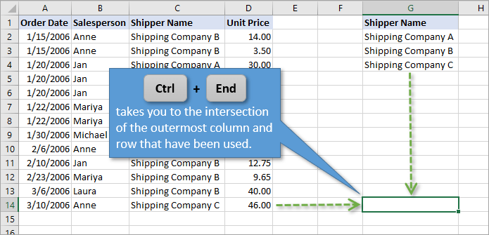
Sometimes, when you use this shortcut, Excel will move your selection so that is farther to the right or farther down than the data range you can see.
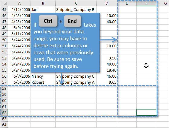
This is usually because there was previously data or formatting in those cells, but it has been deleted. You can clear that by deleting any of those previously used rows or columns and then saving your workbook. (Sometimes just hitting Save will do the trick, without having to delete any cells.)
Ctrl+End will select the last used cell on the sheet. However, there could be shapes (charts, slicers, etc.) on the sheet below or to the right of that cell. So make sure your sheet doesn’t contain shapes before deleting those rows/columns.
2. Select the First Visible Cell
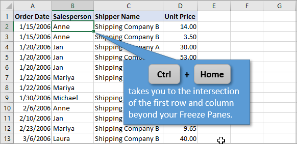
The keyboard shortcut to select the first visible cell on a sheet is: Ctrl+Home
Using Ctrl+Home will always take you to the first visible cell (excluding hidden rows/columns) on the sheet, unless your sheet has Freeze Panes.
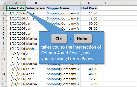
Freeze Panes lock rows and columns in place so that they are always visible, no matter where you scroll to in the worksheet. Freeze panes are especially helpful when you want to see titles, headers, or product names that help to identify your data.
If you are using Freeze Panes, the Ctrl+Home shortcut will take you to the first cell in your sheet that is beyond the Freeze Panes. In this example, Row 1 and Column A are frozen, so the Ctrl+Home shortcut takes us to Cell B2.
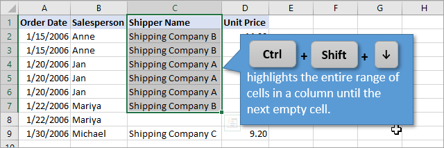
3. Select Last Cell in Contiguous Range
The keyboard shortcut to select the last cell in a contiguous range is:
Ctrl+Arrow Key
Using Ctrl along with your arrow keys allows you to move to the beginning or end of contiguous data in a row or column. For example, if you start at the top of a column and then press Ctrl+? you will jump to the last cell in that column before an empty cell. Repeating this process will move you further down the column to just before the next blank cell.
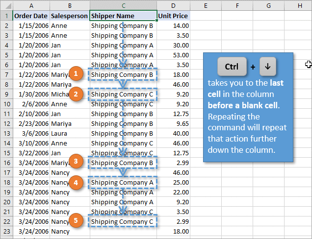
Ctrl+? will reverse that process in the upward direction. And of course, holding Ctrl while using the left or right arrow key accomplishes the same action horizontally instead of vertically.
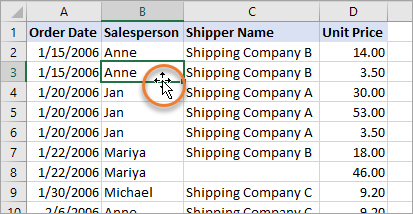
An Alternative Using the Mouse
You can accomplish this same action using your mouse instead of the keyboard, if you like. Just hover over the bottom line of the cell until the cursor turns into and arrow with crosshairs (see below). Then double-click. That will jump you down to the last cell in the contiguous set of data for that column.
4. Add Cells to the Selected Range
The keyboard shortcut to add cells to the selected range is: Shift+Arrow Key
If you use Shift along with your arrow keys, you can select multiple cells, one at a time. For example, if you start in any cell and press Shift+?, it highlights the original cell and the cell just below it.
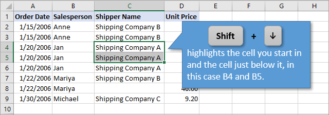
The same idea applies to the left, right, or up arrows. And if you keep the Shift key held down, you can continue to move over multiple cells in multiple directions to select an entire range of data.
5. Select Multiple Cells in Contiguous Range
The keyboard shortcut to select multiple cells in a contiguous range is:
Ctrl+Shift+Arrow Key
Using the same process as in Shortcut 3, but adding the Shift key, allows you to select multiple cells simultaneously. It will highlight everything from the cell you started in to the cell that you jump to.
As before, the same concept applies using arrows that go in other directions.
This process only selects cells that come before a blank cell. However, sometimes a column can have many blank cells. If so, this method may not be your best option. To select large amounts of data containing many blanks, I recommend checking out this post for some alternatives:
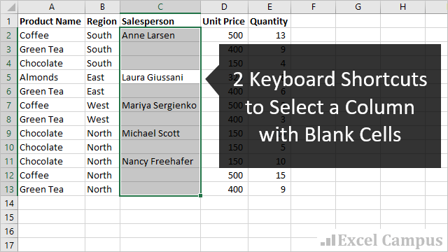
2 Keyboard Shortcuts to Select a Column with Blank Cells
6. Select All Cells to First or Last Cell
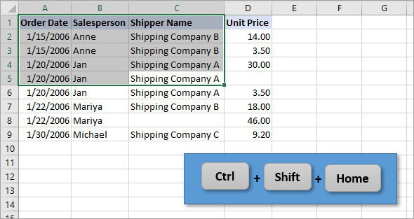
Shortcuts 1 and 2 taught us how to jump from whatever cell we are in to the beginning corner (Home) or ending corner (End) of our data range. Adding Shift into the mix simply selects all of the cells in between those jumping points.
So if, for example, we start in Cell C5 and Press Ctrl+Shift+Home, the following range will be selected.
The keyboard shortcut to all cells to from the active cell to the first visible cell is:
Ctrl+Shift+Home
If instead we were to begin at C5 and press Ctrl+Shift+End, this range of data will be selected:
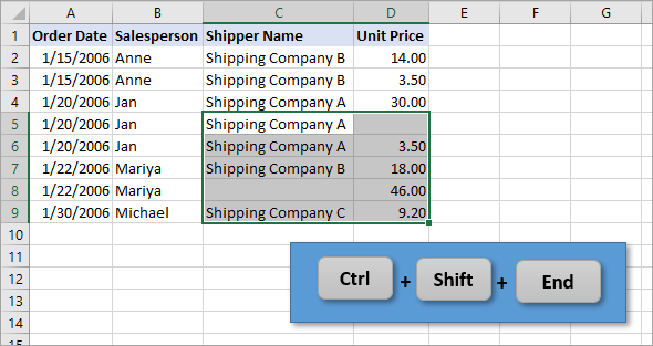
The keyboard shortcut to all cells to from the active cell to the last used cell is:
Ctrl+Shift+End
7. Select All Cells
The keyboard shortcut to all cells in the current used range is: Ctrl+A
Press Ctrl+A a second time to select all cells on the sheet.
If your spreadsheet has multiple blocks of data, Excel does a pretty good job of selecting the block of data that is surrounding your cell when you press Ctrl+A. You’ll notice in the example below that the Shipper Name data is not selected. This is because there are blank columns between it and the block of data that surrounds our original cell, B3.
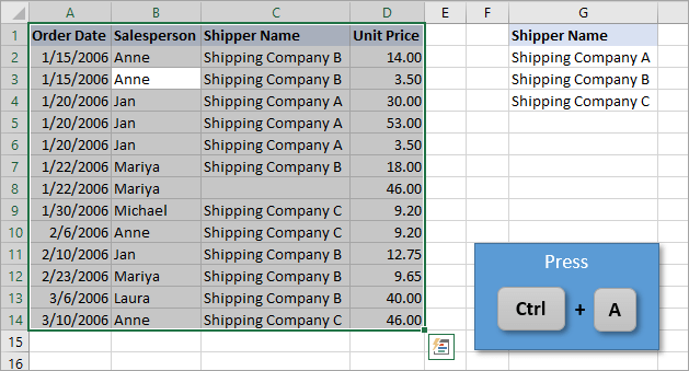
If your intention is to select all of the cells on the sheet, you simply press Ctrl+A a second time and your entire worksheet will be highlighted.
The keyboard shortcut to all cells on the sheet is: Ctrl+A,A
Better, Faster, Smarter
I hope you are able to commit some of these shortcuts to memory. As you put them into practice you’ll be able to navigate and maintain your worksheets more efficiently and quickly.
Have a keyboard shortcut that you want to share? Leave a comment below. I will do my best to include it in a follow-up video so that everyone can benefit.
Asked by: Maurine Greenfelder
Score: 4.8/5
(13 votes)
To do so, follow these steps:
- Start Excel, open your workbook, and then select the range that you want to allow access to.
- In Excel 2007, click the Home tab, click Format in the Cells group, click Format Cells, and then click the Protection tab. …
- Click to clear the Locked check box, and then click OK.
Why won’t Excel let me select a cell?
Extend Selection Mode
If you notice some weird selection behavior going on with your mouse in Excel, take a look at the Status Bar — you might see something toward the left end that says “Extend Selection.” Even if you don’t, turning the selection mode off is easy. Just press F8.
How do I enable cell selection in Excel?
Click the button at the top left corner of worksheet to select all cells. Then press the Ctrl + 1 keys simultaneously to open the Format Cells dialog box. 2. In the Format Cells dialog box, go to the Protection tab, uncheck the Locked box, and then click the OK button.
Can’t select all in Excel?
If you can get your cursor to the end of the text in the cell, try pressing Ctrl + Shift + Home . Alternatively, if you can get your cursor to the start of the text in the cell, try pressing Ctrl + Shift + End .
How do I unlock scroll lock in Excel?
Click Change PC Settings. Select Ease of Access > Keyboard. Click the On Screen Keyboard slider button to turn it on. When the on-screen keyboard appears on your screen, click the ScrLk button.
15 related questions found
How do you remove Scroll Lock in Excel shortcut key?
The fastest way to turn off Screen Lock in Excel is this:
- Click the Windows button and start typing «on-screen keyboard» in the search box. …
- Click the On-Screen Keyboard app to run it.
- The virtual keyboard will show up, and you click the ScrLk key to remove Scroll Lock.
How do I fix scrolling in Excel?
Press Ctrl + Shift + Right Arrow to select all the columns to the right. Then, once again, click Home > Clear > Clear All. Now we have cleared all the unnecessary content, save the document (Ctrl + S). The used range has now been reset, and the scroll bars should return back to a more usable size.
How do I select all text in an Excel cell?
To select all cells on a worksheet, use one of the following methods: Click the Select All button. Press CTRL+A. Note If the worksheet contains data, and the active cell is above or to the right of the data, pressing CTRL+A selects the current region.
How do I select all columns except one in Excel?
Select the header or the first row of your list and press Shift + Ctrl + ↓(the drop down button), then the list has been selected except the first row.
How do you select an entire row in sheets?
Using keyboard shortcuts, To select an entire column press Ctrl + Space . To select an entire row, press Shift + Space . Once a column or row is highlighted, you can apply any properties or changes that can be done to an individual cell.
How do you make a selection in Excel?
Create a drop-down list
- Select the cells that you want to contain the lists.
- On the ribbon, click DATA > Data Validation.
- In the dialog, set Allow to List.
- Click in Source, type the text or numbers (separated by commas, for a comma-delimited list) that you want in your drop-down list, and click OK.
How do you keep a selection in Excel?
Press F8. Use the right arrow and down arrow to move the cursor around, and Excel will keep selecting additional cells until you stop pressing arrow keys.
How do I select only data in a cell in Excel?
Select one or more cells
- Click on a cell to select it. Or use the keyboard to navigate to it and select it.
- To select a range, select a cell, then with the left mouse button pressed, drag over the other cells. …
- To select non-adjacent cells and cell ranges, hold Ctrl and select the cells.
Why can’t I edit my Excel sheet?
If you try to use Edit mode and nothing happens, it might be disabled. You can enable or disable Edit mode by changing an Excel option. Click File > Options > Advanced. , click Excel Options, and then click the Advanced category.
How do you unlock a cell?
Excel 2016: How to Lock or Unlock Cells
- Select the cells you wish to modify.
- Choose the “Home” tab.
- In the “Cells” area, select “Format” > “Format Cells“.
- Select the “Protection” tab.
- Uncheck the box for “Locked” to unlock the cells. Check the box to lock them. Select “OK“.
Is there a unique function in Excel?
The Excel UNIQUE function returns a list of unique values in a list or range. Values can be text, numbers, dates, times, etc. array — Range or array from which to extract unique values.
How do you select all cells below a certain point?
Click on the top cell, then press Ctrl and hold the space bar. All cells beneath the cell initially chosen will be highlighted.
How do I select infinite rows in Excel?
Note If the row or column contains data, CTRL+SHIFT+ARROW key selects the row or column to the last used cell. Pressing CTRL+SHIFT+ARROW key a second time selects the entire row or column.
What is the fastest way to select data in Excel?
7 great keyboard shortcuts for selecting cells quickly.
- Shift + Arrow Keys – Expands the selected range in the direction of the arrow key.
- Shift + Spacebar – Selects the entire row or rows of the selected range.
- Ctrl + Spacebar – Selects the entire column or columns of the selected range.
How do you select cells without dragging?
To select a range of cells without dragging the mouse:
- Click in the cell which is to be one corner of the range of cells.
- Move the mouse to the opposite corner of the range of cells.
- Hold down the Shift key and click.
What is the quickest way to select entire worksheet in Excel?
If you want to quickly select your entire spreadsheet, there are several ways you can do it:
- Click on the button in the upper-left corner of your spreadsheet, where the column and row headers intersect.
- Press Ctrl+Shift+Space Bar.
- Press Ctrl+A.
Why does my Excel keep scrolling?
I’m happy to work with you on this issue. To turn it off in Excel, see the Troubleshooting Scroll Lock, right click on the bottom bar (Excel status bar) and untick scroll lock. This will stop auto scrolling, and of course you can always turn it back on after. You may refer to the link below for more details.
Why is my Excel scrolling instead of moving cells?
When the arrow keys scroll through your entire spreadsheet rather than moving from cell to cell, the culprit of this behavior is the Scroll Lock key. … If you don’t know what you accidentally pressed, you can turn Scroll Lock off using the on-screen keyboard.
Why scroll down is not working in Excel?
Re: My excel spreadsheet won’t scroll down
You can normally toggle Scroll Lock off and on by hitting the Scroll Lock key on your keyboard. If you don’t have a scroll lock key on your keyboard do this… … That should bring up the on-screen keyboard, click on the «scroll lock» key to toggle off that option.