
If you look carefully you’ll see that one of the dates is the 29th of February 2018, which isn’t a valid date. This was most likely a data entry error.
Pivot tables won’t allow you to group dates if there are any invalid dates within the data source. Blank cells are also considered to be invalid dates, so you must make sure that there are no blanks. If you fix your data so that there are no invalid values, the error should disappear and you should be able to group your pivot table.
Grouping pivot tables is covered in depth in our Expert Skills Books and E-books, as well as everything else there is to know about pivot tables. If you need to improve your knowledge of pivot tables and other advanced Excel features it could be of great value to you.
If you’re an Excel beginner you might find our free Basic Skills E-book useful, or our complete Essential Skills Books and E-books.
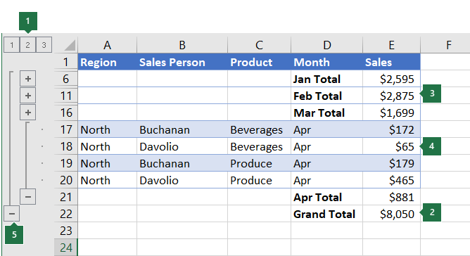
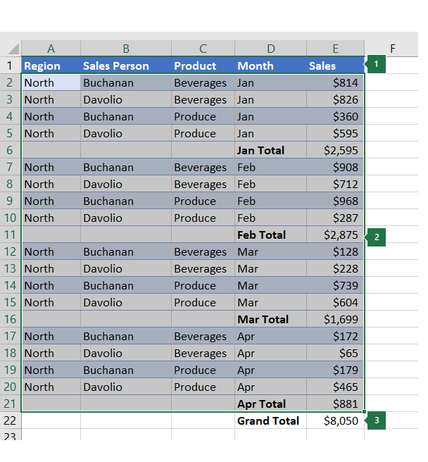
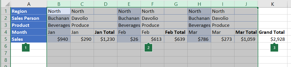
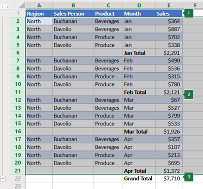
If you have a list of data you want to group and summarize, you can create an outline of up to eight levels. Each inner level, represented by a higher number in the outline symbols, displays detail data for the preceding outer level, represented by a lower number in the outline symbols. Use an outline to quickly display summary rows or columns, or to reveal the detail data for each group. You can create an outline of rows (as shown in the example below), an outline of columns, or an outline of both rows and columns.
|
|
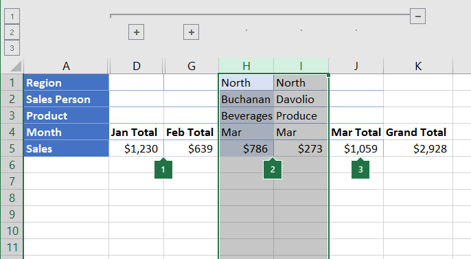
1. To display rows for a level, click the appropriate 2. Level 1 contains the total sales for all detail rows. 3. Level 2 contains total sales for each month in each region. 4. Level 3 contains detail rows — in this case, rows 17 through 20. 5. To expand or collapse data in your outline, click the |
 outline symbols.
 and
and  outline symbols, or press ALT+SHIFT+= to expand and ALT+SHIFT+- to collapse.
-
Make sure that each column of the data that you want to outline has a label in the first row (e.g., Region), contains similar facts in each column, and that the range you want to outline has no blank rows or columns.
-
If you want, your grouped detail rows can have a corresponding summary row—a subtotal. To create these, do one of the following:
-
Insert summary rows by using the Subtotal command
Use the Subtotal command, which inserts the SUBTOTAL function immediately below or above each group of detail rows and automatically creates the outline for you. For more information about using the Subtotal function, see SUBTOTAL function.
-
Insert your own summary rows
Insert your own summary rows, with formulas, immediately below or above each group of detail rows. For example, under (or above) the rows of sales data for March and April, use the SUM function to subtotal the sales for those months. The table later in this topic shows you an example of this.
-
-
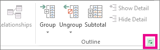
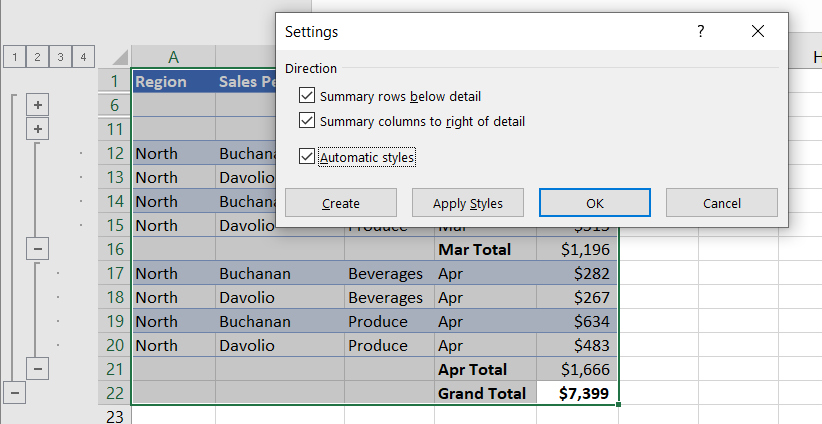
By default, Excel looks for summary rows below the details they summarize, but it’s possible to create them above the detail rows. If you created the summary rows below the details, skip to the next step (step 4). If you created your summary rows above your detail rows, on the Data tab, in the Outline group, click the dialog box launcher.

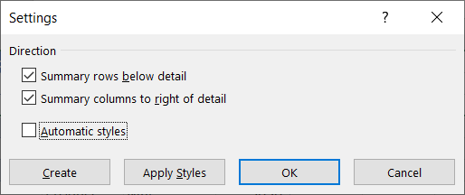
The Settings dialog box opens.
Then in the Settings dialog box, clear the Summary rows below detail checkbox, and then click OK.
-
Outline your data. Do one of the following:
Outline the data automatically
-
Select a cell in the range of cells you want to outline.
-
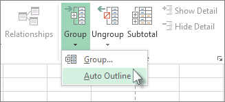
On the Data tab, in the Outline group, click the arrow under Group, and then click Auto Outline.
Outline the data manually
Important: When you manually group outline levels, it’s best to have all data displayed to avoid grouping the rows incorrectly.
-
To outline the outer group (level 1), select all of the rows the outer group will contain (i.e., the detail rows and if you added them, their summary rows).
1. The first row contains labels, and is not selected.
2. Since this is the outer group, select all the rows with subtotals and details.
3. Don’t select the grand total.
-
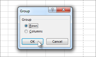
On the Data tab, in the Outline group, click Group. Then in the Group dialog box, click Rows, and then click OK.
Tip: If you select entire rows instead of just the cells, Excel automatically groups by row — the Group dialog box doesn’t even open.
The outline symbols appear beside the group on the screen.
-
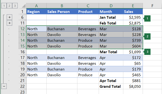
Optionally, outline an inner, nested group — the detail rows for a given section of your data.
Note: If you don’t need to create any inner groups, skip to step f, below.
For each inner, nested group, select the detail rows adjacent to the row that contains the summary row.
1. You can create multiple groups at each inner level. Here, two sections are already grouped at level 2.
2. This section is selected and ready to group.
3. Don’t select the summary row for the data you are grouping.
-
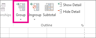
On the Data tab, in the Outline group, click Group.
Then in the Group dialog box, click Rows, and then click OK. The outline symbols appear beside the group on the screen.
Tip: If you select entire rows instead of just the cells, Excel automatically groups by row — the Group dialog box doesn’t even open.
-
Continue selecting and grouping inner rows until you have created all of the levels that you want in the outline.
-
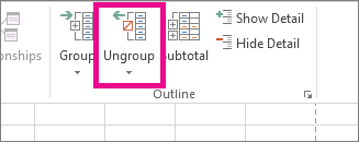
If you want to ungroup rows, select the rows, and then on the Data tab, in the Outline group, click Ungroup.
You can also ungroup sections of the outline without removing the entire level. Hold down SHIFT while you click the
or for the group, and then on the Data tab, in the Outline group, click Ungroup.Important: If you ungroup an outline while the detail data is hidden, the detail rows may remain hidden. To display the data, drag across the visible row numbers adjacent to the hidden rows. Then on the Home tab, in the Cells group, click Format, point to Hide & Unhide, and then click Unhide Rows.
-
-
Make sure that each row of the data that you want to outline has a label in the first column, contains similar facts in each row, and the range has no blank rows or columns.
-
Insert your own summary columns with formulas immediately to the right or left of each group of detail columns. The table listed in step 4 below shows you an example.
Note: To outline data by columns, you must have summary columns that contain formulas that reference cells in each of the detail columns for that group.
-
If your summary column is to the left of the detail columns, on the Data tab, in the Outline group, click the dialog box launcher.
The Settings dialog box opens.
Then in the Settings dialog box, clear the Summary columns to right of detail check box, and click OK.
-
To outline the data, do one of the following:
Outline the data automatically
-
Select a cell in the range.
-
On the Data tab, in the Outline group, click the arrow below Group and click Auto Outline.
Outline the data manually
Important: When you manually group outline levels, it’s best to have all data displayed to avoid grouping columns incorrectly.
-
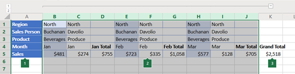
To outline the outer group (level 1), select all of the subordinate summary columns, as well as their related detail data.
1. Column A contains labels.
2. Select all the detail and subtotal columns. Note that if you don’t select entire columns, when you click Group (on the Data tab in the Outline group) the Group dialog box will open and ask you to choose Rows or Columns.
3. Don’t select the grand total column.
-
On the Data tab, in the Outline group, click Group.
The outline symbol appears above the group.
-
To outline an inner, nested group of detail columns (level 2 or higher), select the detail columns adjacent to the column that contains the summary column.
1. You can create multiple groups at each inner level. Here, two sections are already grouped at level 2.
2. These columns are selected and ready to group. Note that if you don’t select entire columns, when you click Group (on the Data tab in the Outline group) the Group dialog box will open and ask you to choose Rows or Columns.
3. Don’t select the summary column for the data you are grouping.
-
On the Data tab, in the Outline group, click Group.
The outline symbols appear beside the group on the screen.
-
-
Continue selecting and grouping inner columns until you have created all of the levels that you want in the outline.
-
If you want to ungroup columns, select the columns, and then on the Data tab, in the Outline group, click Ungroup.
You can also ungroup sections of the outline without removing the entire level. Hold down SHIFT while you click the  or
or  for the group, and then on the Data tab, in the Outline group, click Ungroup.
If you ungroup an outline while the detail data is hidden, the detail columns may remain hidden. To display the data, drag across the visible column letters adjacent to the hidden columns. On the Home tab, in the Cells group, click Format, point to Hide & Unhide, and then click Unhide Columns
-
If you don’t see the outline symbols
, , and , go to File > Options > Advanced, and then under the Display options for this worksheet section, select the Show outline symbols if an outline is applied check box, and then click OK. -
Do one or more of the following:
-
Show or hide the detail data for a group
To display the detail data within a group, click the
button for the group, or press ALT+SHIFT+=. -
To hide the detail data for a group, click the
button for the group, or press ALT+SHIFT+-. -
Expand or collapse the entire outline to a particular level
In the
outline symbols, click the number of the level that you want. Detail data at lower levels is then hidden.For example, if an outline has four levels, you can hide the fourth level while displaying the rest of the levels by clicking
. -
Show or hide all of the outlined detail data
To show all detail data, click the lowest level in the
outline symbols. For example, if there are three levels, click . -
To hide all detail data, click
.
-
 .
. .
.For outlined rows, Microsoft Excel uses styles such as RowLevel_1 and RowLevel_2 . For outlined columns, Excel uses styles such as ColLevel_1 and ColLevel_2. These styles use bold, italic, and other text formats to differentiate the summary rows or columns in your data. By changing the way each of these styles is defined, you can apply different text and cell formats to customize the appearance of your outline. You can apply a style to an outline either when you create the outline or after you create it.
Do one or more of the following:
Automatically apply a style to new summary rows or columns
-
On the Data tab, in the Outline group, click the dialog box launcher.
The Settings dialog box opens.
-
Select the Automatic styles check box.
Apply a style to an existing summary row or column
-
Select the cells to which you want to apply a style.
-
On the Data tab, in the Outline group, click the dialog box launcher.
The Settings dialog box opens.
-
Select the Automatic styles check box, and then click Apply Styles.
You can also use autoformats to format outlined data.
-
If you don’t see the outline symbols
, , and , go to File > Options > Advanced, and then under the Display options for this worksheet section, select the Show outline symbols if an outline is applied check box. -
Use the outline symbols
, , and to hide the detail data that you don’t want copied.For more information, see the section, Show or hide outlined data.
-
Select the range of summary rows.
-
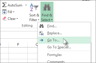
On the Home tab, in the Editing group, click Find & Select, and then click Go To.
-
Click Go To Special.
-
Click Visible cells only.
-
Click OK, and then copy the data.
Note: No data is deleted when you hide or remove an outline.
Hide an outline
-
Go to File > Options > Advanced, and then under the Display options for this worksheet section, uncheck the Show outline symbols if an outline is applied check box.
Remove an outline
-
Click the worksheet.
-
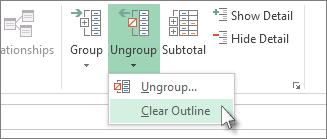
One the Data tab, in the Outline group, click Ungroup and click Clear Outline.
Important: If you remove an outline while the detail data is hidden, the detail rows or columns may remain hidden. To display the data, drag across the visible row numbers or column letters adjacent to the hidden rows and columns. On the Home tab, in the Cells group, click Format, point to Hide & Unhide, and then click Unhide Rows or Unhide Columns.
Imagine that you want to create a summary report of your data that only displays totals accompanied by a chart of those totals. In general, you can do the following:
-
Create a summary report
-
Outline your data.
For more information, see the sections Create an outline of rows or Create an outline of columns.
-
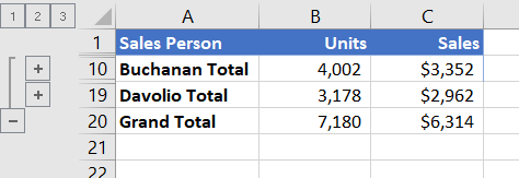
Hide the detail by clicking the outline symbols
, , and to show only the totals as shown in the following example of a row outline:
-
For more information, see the section, Show or hide outlined data.
-
-
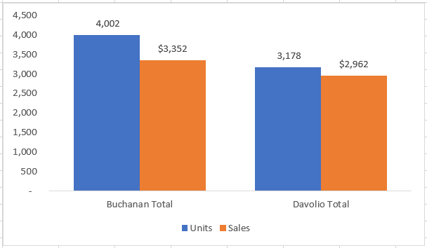
Chart the summary report
-
Select the summary data that you want to chart.
For example, to chart only the Buchanan and Davolio totals, but not the grand totals, select cells A1 through C19 as shown in the above example.
-
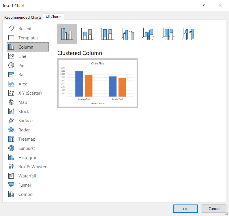
Click Insert > Charts > Recommended Charts, then click the All Charts tab and choose your chart type.
For example, if you chose the Clustered Column option, your chart would look like this:
If you show or hide details in the outlined list of data, the chart is also updated to show or hide the data.
-
You can group (or outline) rows and columns in Excel for the web.
Note: Although you can add summary rows or columns to your data (by using functions such as SUM or SUBTOTAL), you cannot apply styles or set a position for summary rows and columns in Excel for the web.
Create an outline of rows or columns
|
|
|
|
Outline of rows in Excel Online
|
Outline of columns in Excel Online
|
-
Make sure that each column (or row) of the data that you want to outline has a label in the first row (or column), contains similar facts in each column (or row), and that the range has no blank rows or columns.
-
Select the data (including any summary rows or columns).
-
On the Data tab, in the Outline group, click Group > Group Rows or Group Columns.
-
Optionally, if you want to outline an inner, nested group — select the rows or columns within the outlined data range, and repeat step 3.
-
Continue selecting and grouping inner rows or columns until you have created all of the levels that you want in the outline.
Ungroup rows or columns
-
To ungroup, select the rows or columns, and then on the Data tab, in the Outline group, click Ungroup and select Ungroup Rows or Ungroup Columns.
Show or hide outlined data
Do one or more of the following:
Show or hide the detail data for a group
-
To display the detail data within a group, click the
for the group, or press ALT+SHIFT+=. -
To hide the detail data for a group, click the
for the group, or press ALT+SHIFT+-.
Expand or collapse the entire outline to a particular level
-
In the
outline symbols, click the number of the level that you want. Detail data at lower levels is then hidden. -
For example, if an outline has four levels, you can hide the fourth level while displaying the rest of the levels by clicking
.
Show or hide all of the outlined detail data
-
To show all detail data, click the lowest level in the
outline symbols. For example, if there are three levels, click . -
To hide all detail data, click
.
Need more help?
You can always ask an expert in the Excel Tech Community or get support in the Answers community.
See Also
Group or ungroup data in a PivotTable
When you try to group dates in an Excel pivot table, or other pivot table items, you might get a pivot table error, “Cannot group that selection.” In Excel 2010, and earlier versions, that error was usually caused by blank cells in your source data, or text in the number or date columns. If you’re using Excel 2013 or later, there’s another reason that might prevent you from grouping pivot table items.
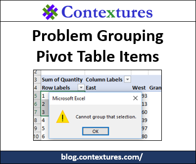
Cannot Group That Selection
Here’s a screen shot of the pivot table error, “Cannot group that selection.” that appears. As you can see, the error message doesn’t tell you WHY you can’t group the items. Excel leaves it up to you to find out what the problem is.

Data Model
You can run into pivot table grouping problems in any version of Excel. But if you’re using Excel 2013 or later, there’s a new reason for the error message, that might affect you. Here’s what can happen:
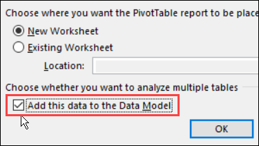
- When you create a pivot table, there’s a check box to “Add this data to the Data Model”.
- If you checked that box, you won’t be able to group any items in the pivot table.
OLAP-Based Pivot Table
If you added the source data to the data model, you created an OLAP-based Power Pivot, instead of a traditional (normal) pivot table. In OLAP-based pivot tables, the grouping feature is not available.
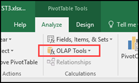
A quick way to tell if your pivot table is OLAP-based is to check the Ribbon:
- Select any cell in the pivot table
- On the Excel Ribbon, click the Analyze tab (under PivotTable Tools)
- In the Calculations section, find the OLAP Tools command.
- If it’s dimmed out, your pivot table is the traditional type
- If the command is active, your pivot table is OLAP-based
Limitations in OLAP-Based Pivot Tables
It’s not just grouping that is prevented In OLAP-based pivot tables. Other features are unavailable too.
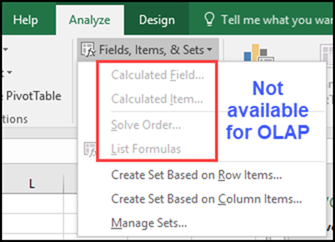
For example, you can’t create a calculated field or calculated item.
No Fix for this Grouping Problem
Unfortunately, there’s no fix for grouping in an OLAP-based pivot table. If you want grouping, you’ll need a pivot table with its source data NOT added to the data model.
To get grouping:
- Create a second pivot table from the source data
- Do NOT check the box to add the data to the Data Model.
Keep the OLAP-based pivot table too, and you’ll have two pivot tables based on the same data, using different pivot caches.
NOTE: There’s no option or setting that lets you change the pivot table from an OLAP-based source (data model), to a data source that isn’t in the data model.
Grouping Error for Normal Pivot Tables
If your pivot table is the traditional type (not in the data model), grouping problems are usually caused by invalid data in the field that you’re trying to group.
For solutions to grouping error in Normal Pivot Tables, see the Pivot Table Grouping page on my Contextures website.
Videos: Pivot Table Grouping
Learn more about pivot table grouping, and get a workbook with sample file that you can use for testing. Go to the How to Group Pivot Table Data page on my Contextures website.
This short video shows the basics of pivot table grouping
This video shows how to group Text items in a pivot table.
Related Articles
Pivot Table Grouping Affects Another Pivot Table
Stop Pivot Table Date Grouping
Grouping Pivot Table Dates by Fiscal Year
Grouping Pivot Table Dates by Months and Weeks
______________________
Excel Pivot Table Error Cannot Group That Selection

__________________
If you try to group pivot table items in Excel, you might get an error message that says, “Cannot group that selection.” For older versions of Excel, if you had a problem grouping pivot table items, it was usually caused by blank cells, or text in number/date fields. For Excel 2013 and later, there’s another thing that can prevent you from grouping — the Excel Data Model.
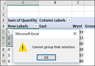
Cannot Group That Selection
Here’s a screen shot of the “Cannot group that selection.” error message that appears. The message doesn’t give you any clues as to why you can’t group the items. It’s up to you to do the detective work.
Data Model
We’ll look at the traditional reasons for this grouping problem in the next section. But first, here’s the newer issue, that might affect you, if you’re using Excel 2013 or later.
- When you create a pivot table, there’s a check box to “Add this data to the Data Model”.
- If you checked that box, you won’t be able to group any items in the pivot table.
When the source data is added to the data model, you end up with an OLAP-based Power Pivot, instead of a traditional pivot table, and the grouping feature is not available.
Is It OLAP-Based?
A quick way to tell if your pivot table is OLAP-based is to check the Ribbon:
Select any cell in the pivot table
- On the Excel Ribbon, click the Analyze tab (under PivotTable Tools)
- In the Calculations section, find the OLAP Tools command.
- If it’s dimmed out, your pivot table is the traditional type
- If the command is active, your pivot table is OLAP-based
And if you check the Fields, Items, & Sets drop down, some of the features will be dimmed out, for OLAP-based pivot tables. For example, you can’t create a calculated field or calculated item.
Fix the Grouping Problem
I haven’t found any way to change the pivot cache from an OLAP-based source (data model), to a data source that isn’t in the data model. So, if you need grouping, create a new pivot table from the source data, and do NOT check the box to add the data to the Data Model.
NOTE: You can keep the OLAP-based pivot table too, and have two pivot tables based on the same data, using different pivot caches.
Blank Cells or Text
If your pivot table is the traditional type (not in the data model), grouping problems are usually caused by invalid data in the field that you’re trying to group.
If you’re trying to group dates or numbers, the grouping problem usually occurs when the field contains records with one of these items:
- a blank cell in a date/number field, or
- a text entry in a date/number field.
To fix the problem
- For blank cells, fill in the date/number (use a dummy date/number if necessary).
- If there is text in the date/number field, remove it.
- If numbers are being recognized as text, use one of the techniques to change text to real numbers.
Then refresh the pivot table, and try grouping the items again.
Previous Grouping
If you don’t have blank cells or text in the date column, there may be a grouped field left over from a previous time that you grouped the data.
- Check the field list, to see if there’s a second copy of the date field, e.g. Date2.
- If there is, add it to the row area, and ungroup it.
- Then, you should be able to group the date field again.
Videos: Pivot Table Grouping
Learn more about pivot table grouping, and get a workbook with sample file that you can use for testing. Go to the How to Group Pivot Table Data page on my Contextures website.
This short video shows the basics of pivot table grouping
This video shows how to group Text items in a pivot table.
More Pivot Table Links
Clear Old Items in Pivot Table
Calculated Field – Count
Calculated Items
Summary Functions
_____________________________

_____________________________
Excel Pivot Table Date Grouping is a very powerful feature in Excel that allows you to quickly group dates into years, quarters, months, weeks, days, hours, minutes and/or seconds.
However, there are times when Excel Pivot Table dates cannot group that selection and we get an error message: Cannot group that selection.

Instead of checking the dates one by one to find out where the error occurred, I will show you a quick way to fix the Cannot group that selection error message!
In this article, you will go through a detailed guide on:
- How to Group Dates in Excel
- Reasons for Cannot Group That Selection Error in Excel Pivot Table Date Grouping
- Quick ways to Fix the Cannot Group That Selection Error
Let’s discuss each of these points one after the other!
How to Group Dates in Excel
In the table below, you have a Pivot Table created with the sales amount for each individual day.
To learn how to create a Pivot Table in Excel – Click Here.

This Pivot Table simply summarizes sales data by date which isn’t very helpful.
You might want to see the total sales achieved per month, week, or year. Using formulas or VBA to get the work done will be too complicated.
Want an Easy Fix?? Try Excel Pivot Table Date Grouping!!
Follow the steps below to understand how to Group Dates in Excel Pivot Table:
STEP 1: Right-Click on the Date field in the Pivot Table.

STEP 2: Select the option – Group

STEP 3: In the dialog box, select one or more options as per your requirement.
To Group Dates by Year and Month.
- Select Month & Year. Click OK.

STEP 4: Your Pivot Table with Grouped Dates by Year & Month is ready!

To group data by week,
- Select Days
- Type Number of days as 7

Your Grouped Dates by Week is ready!

Another way to access the Grouping dialog box, Go to Pivot Table Tools > Analyze > Group Selection

Reasons for “Cannot group that selection” Error in Excel Pivot Table Date Grouping
The most common reason for facing this issue is that the date column contains either
- Is Blank
- Contains Text
- Contains an Error.
If even one of the cells contains invalid data, the grouping feature will not be enabled.
Pivot Table won’t allow you to group dates and you will get a cannot group that selection error.
So, the ideal step would be to look for those cells and fix them!
Below are the 2 Quick and Easy methods to find the cells containing invalid data and disappear the errors!
Quick ways to Fix the “Cannot group that selection” Error
In the example below I show you how to get the Errors when Grouping By Dates:

Follow the step-by-step tutorial on how to fix error in Excel Pivot Table Date Grouping and make sure to download the Excel Workbook and follow along:
METHOD 1:
STEP 1: Right-click on any row in your Pivot Table and select Group so we can select our Group type that we want:

However, we notice that we have an error!
STEP 2: To check where our error occurred, go to the data table and highlight the column that contains our dates.

STEP 3: Go to Home > Find & Select > Go To Special:

Make sure the Constants, Text, and Errors are selected. This will select all our invalid dates (Errors) and text data (Text).

STEP 4: Excel has now selected the incorrect dates. To make each incorrect cell easier to view go to Home > Fill Color

The invalid dates are now highlighted:

STEP 5: Manually replace the incorrect dates with the correct dates:

STEP 6: We need to Refresh our pivot table to load our new correct dates but first we need to “uncheck” the ORDER DATE field.

Right-click on the Pivot Table and click Refresh:

“Check” the ORDER DATE Field:

STEP 7: Right-click on the Pivot Table and click Group:

The Excel Pivot Table Date Grouping is now displayed! Your data is now clean!

Your Grouped Data looks like this:

METHOD 2:
If you look at the Data Table, one of the cells contains a Date with incorrect format (Excel stores it as text) and a Text Value.

When you try to Group this Data, you will see that Excel Pivot Table not grouping dates and will display this Cannot group that selection error.
Now, to fix this you can simply use the filter button to find the cells containing incorrect format or text.
STEP 1: Go to Data > Filter icon

STEP 2: In the Filter dropdown, you will be able to easily spot these cells.
Select only those values.

Click OK.

STEP 3: Fix the error in those cells.
STEP 4: Go back to the Pivot Table, Select PivotTable Analyze > Refresh.

STEP 5: Try grouping the data again. Voila! It’s done now.
Conclusion
In this article, you have learned how to group dates in an Excel Pivot Table and fix the cannot group that selection error when the Pivot Table group by month is not working.
Did you know there are many creative ways of doing grouping in Excel Pivot Tables? Learn all about it here!
Make sure to download our FREE PDF on the 333 Excel keyboard Shortcuts here:

You can learn more about how to use Excel by viewing our FREE Excel webinar training on Formulas, Pivot Tables, and Macros & VBA!
