
Excel for Microsoft 365 Excel for Microsoft 365 for Mac Excel for the web Excel 2021 Excel 2021 for Mac Excel 2019 Excel 2019 for Mac Excel 2016 Excel 2016 for Mac Excel 2013 Excel for iPad Excel for iPhone Excel for Android tablets Excel 2010 Excel 2007 Excel for Mac 2011 Excel for Android phones Excel Mobile Excel Starter 2010 More…Less
When you need to perform simple arithmetic calculations on several ranges of cells, sum the results, and use criteria to determine which cells to include in the calculations, consider using the SUMPRODUCT function.
SUMPRODUCT takes arrays and arithmetic operators as arguments. You can use arrays that evaluate as True or False (1 or 0) as criteria by using them as factors (multiplying them by the other arrays).
For example, suppose you want to calculate net sales for a particular sales agent by subtracting expenses from gross sales, as in this example.

-
Click a cell outside the ranges you are evaluating. This is where your result goes.
-
Type =SUMPRODUCT(.
-
Type (, enter or select a range of cells to include in your calculations, then type ). For example, to include the column Sales from the table Table1, type (Table1[Sales]).
-
Enter an arithmetic operator: *, /, +, —. This is the operation you will perform using the cells that meet any criteria you include; you can include more operators and ranges. Multiplication is the default operation.
-
Repeat steps 3 and 4 to enter additional ranges and operators for your calculations. After you add the last range you want to include in calculations, add a set of parentheses enclosing all the involved ranges, so that the entire calculation is enclosed. For example, ((Table1[Sales])+(Table1[Expenses])).
You may need to include additional parentheses inside your calculation to group various elements, depending on the arithmetic you want to perform.
-
To enter a range to use as a criterion, type *, enter the range reference normally, then after the range reference but before the right parenthesis, type =», then the value to match, then «. For example, *(Table1[Agent]=»Jones»). This causes the cells to evaluate as 1 or 0, so when multiplied by other values in the formula the result is either the same value or zero — effectively including or excluding the corresponding cells in any calculations.
-
If you have more criteria, repeat step 6 as needed. After your last range, type ).
Your completed formula might look like the one in our example above: =SUMPRODUCT(((Table1[Sales])-(Table1[Expenses]))*(Table1[Agent]=B8)), where cell B8 holds the agent name.
Need more help?
Want more options?
Explore subscription benefits, browse training courses, learn how to secure your device, and more.
Communities help you ask and answer questions, give feedback, and hear from experts with rich knowledge.
There are many ways to force excel for calculating a formula only if given cell/s are not blank. In this article, we will explore all the methods of calculating only «if not blank» condition.
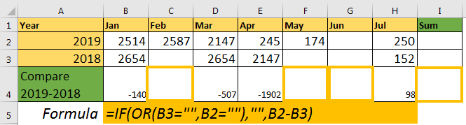
So to demonstrate all the cases, I have prepared below data

In row 4, I want the difference of months of years 2109 and 2018. For that, I will subtract 2018’s month’s data from 2019’s month’s data. The condition is, if either cell is blank, there should be no calculation. Let’s explore in how many ways you can force excel, if cell is not blank.
Calculate If Not Blank using IF function with OR Function.
The first function we think of is IF function, when it comes to conditional output. In this example, we will use IF and OR function together.
So if you want to calculate if all cells are non blank then use below formula.
Write this formula in cell B4 and fill right (CTRL+R).
=IF(OR(B3=»»,B2=»»),»»,B2-B3)
How Does It work?
The OR function checks if B3 and B2 are blank or not. If either of the cell is blank, it returns TRUE. Now, for True, IF is printing “” (nothing/blank) and for False, it is printing the calculation.
The same thing can be done using IF with AND function, we just need to switch places of True Output and False Output.
=IF(AND(B3<>»»,B2<>»»),B2-B3,»»)
In this case, if any of the cells is blank, AND function returns false. And then you know how IF treats the false output.
Using the ISBLANK function
In the above formula, we are using cell=”” to check if the cell is blank or not. Well, the same thing can be done using the ISBLANK function.
=IF(OR(ISBLANK(B3),ISBLANK(B2)),””,B2-B3)
It does the same “if not blank then calculate” thing as above. It’s just uses a formula to check if cell is blank or not.
Calculate If Cell is Not Blank Using COUNTBLANK
In above example, we had only two cells to check. But what if we want a long-range to sum, and if the range has any blank cell, it should not perform calculation. In this case we can use COUNTBLANK function.
=IF(COUNTBLANK(B2:H2),»»,SUM(B2:H2))
Here, count blank returns the count blank cells in range(B2:H2). In excel, any value grater then 0 is treated as TRUE. So, if ISBLANK function finds a any blank cell, it returns a positive value. IF gets its check value as TRUE. According to the above formula, if prints nothing, if there is at least one blank cell in the range. Otherwise, the SUM function is executed.
Using the COUNTA function
If you know, how many nonblank cells there should be to perform an operation, then COUNTA function can also be used.
For example, in range B2:H2, I want to do SUM if none of the cells are blank.
So there is 7 cell in B2:H2. To do calculation only if no cells are blank, I will write below formula.
=IF(COUNTA(B3:H3)=7,SUM(B3:H3),»»)
As we know, COUNTA function returns a number of nonblank cells in the given range. Here we check the non-blank cell are 7. If they are no blank cells, the calculation takes place otherwise not.
This function works with all kinds of values. But if you want to do operation only if the cells have numeric values only, then use COUNT Function instead.
So, as you can see that there are many ways to achieve this. There’s never only one path. Choose the path that fits for you. If you have any queries regarding this article, feel free to ask in the comments section below.
Related Articles:
How to Calculate Only If Cell is Not Blank in Excel
Adjusting a Formula to Return a Blank
Checking Whether Cells in a Range are Blank, and Counting the Blank Cells
SUMIF with non-blank cells
Only Return Results from Non-Blank Cells
Popular Articles
50 Excel Shortcut to Increase Your Productivity : Get faster at your task. These 50 shortcuts will make you work even faster on Excel.
How to use the VLOOKUP Function in Excel : This is one of the most used and popular functions of excel that is used to lookup value from different ranges and sheets.
How to use the COUNTIF function in Excel : Count values with conditions using this amazing function. You don’t need to filter your data to count specific values. Countif function is essential to prepare your dashboard.
How to use the SUMIF Function in Excel : This is another dashboard essential function. This helps you sum up values on specific conditions.
Excel has a number of formulas that help you use your data in useful ways. For example, you can get an output based on whether or not a cell meets certain specifications. Right now, we’ll focus on a function called “if cell contains, then”. Let’s look at an example.
Jump To Specific Section:
- Explanation: If Cell Contains
- If cell contains any value, then return a value
- If cell contains text/number, then return a value
- If cell contains specific text, then return a value
- If cell contains specific text, then return a value (case-sensitive)
- If cell does not contain specific text, then return a value
- If cell contains one of many text strings, then return a value
- If cell contains several of many text strings, then return a value
Excel Formula: If cell contains
Generic formula
=IF(ISNUMBER(SEARCH("abc",A1)),A1,"")
Summary
To test for cells that contain certain text, you can use a formula that uses the IF function together with the SEARCH and ISNUMBER functions. In the example shown, the formula in C5 is:
=IF(ISNUMBER(SEARCH("abc",B5)),B5,"")
If you want to check whether or not the A1 cell contains the text “Example”, you can run a formula that will output “Yes” or “No” in the B1 cell. There are a number of different ways you can put these formulas to use. At the time of writing, Excel is able to return the following variations:
- If cell contains any value
- If cell contains text
- If cell contains number
- If cell contains specific text
- If cell contains certain text string
- If cell contains one of many text strings
- If cell contains several strings
Using these scenarios, you’re able to check if a cell contains text, value, and more.
Explanation: If Cell Contains
One limitation of the IF function is that it does not support Excel wildcards like «?» and «*». This simply means you can’t use IF by itself to test for text that may appear anywhere in a cell.
One solution is a formula that uses the IF function together with the SEARCH and ISNUMBER functions. For example, if you have a list of email addresses, and want to extract those that contain «ABC», the formula to use is this:
=IF(ISNUMBER(SEARCH("abc",B5)),B5,""). Assuming cells run to B5
If «abc» is found anywhere in a cell B5, IF will return that value. If not, IF will return an empty string («»). This formula’s logical test is this bit:
ISNUMBER(SEARCH("abc",B5))
Read article: Excel efficiency: 11 Excel Formulas To Increase Your Productivity
Using “if cell contains” formulas in Excel
The guides below were written using the latest Microsoft Excel 2019 for Windows 10. Some steps may vary if you’re using a different version or platform. Contact our experts if you need any further assistance.
1. If cell contains any value, then return a value
This scenario allows you to return values based on whether or not a cell contains any value at all. For example, we’ll be checking whether or not the A1 cell is blank or not, and then return a value depending on the result.
- Select the output cell, and use the following formula: =IF(cell<>»», value_to_return, «»).
- For our example, the cell we want to check is A2, and the return value will be No. In this scenario, you’d change the formula to =IF(A2<>»», «No», «»).
- Since the A2 cell isn’t blank, the formula will return “No” in the output cell. If the cell you’re checking is blank, the output cell will also remain blank.
2. If cell contains text/number, then return a value
With the formula below, you can return a specific value if the target cell contains any text or number. The formula will ignore the opposite data types.
Check for text
- To check if a cell contains text, select the output cell, and use the following formula: =IF(ISTEXT(cell), value_to_return, «»).
- For our example, the cell we want to check is A2, and the return value will be Yes. In this scenario, you’d change the formula to =IF(ISTEXT(A2), «Yes», «»).

- Because the A2 cell does contain text and not a number or date, the formula will return “Yes” into the output cell.
Check for a number or date
- To check if a cell contains a number or date, select the output cell, and use the following formula: =IF(ISNUMBER(cell), value_to_return, «»).
- For our example, the cell we want to check is D2, and the return value will be Yes. In this scenario, you’d change the formula to =IF(ISNUMBER(D2), «Yes», «»).

- Because the D2 cell does contain a number and not text, the formula will return “Yes” into the output cell.
3. If cell contains specific text, then return a value
To find a cell that contains specific text, use the formula below.
- Select the output cell, and use the following formula: =IF(cell=»text», value_to_return, «»).
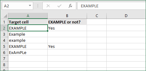
- For our example, the cell we want to check is A2, the text we’re looking for is “example”, and the return value will be Yes. In this scenario, you’d change the formula to =IF(A2=»example», «Yes», «»).

- Because the A2 cell does consist of the text “example”, the formula will return “Yes” into the output cell.
4. If cell contains specific text, then return a value (case-sensitive)
To find a cell that contains specific text, use the formula below. This version is case-sensitive, meaning that only cells with an exact match will return the specified value.
- Select the output cell, and use the following formula: =IF(EXACT(cell,»case_sensitive_text»), «value_to_return», «»).
- For our example, the cell we want to check is A2, the text we’re looking for is “EXAMPLE”, and the return value will be Yes. In this scenario, you’d change the formula to =IF(EXACT(A2,»EXAMPLE»), «Yes», «»).
- Because the A2 cell does consist of the text “EXAMPLE” with the matching case, the formula will return “Yes” into the output cell.
5. If cell does not contain specific text, then return a value
The opposite version of the previous section. If you want to find cells that don’t contain a specific text, use this formula.
- Select the output cell, and use the following formula: =IF(cell=»text», «», «value_to_return»).
- For our example, the cell we want to check is A2, the text we’re looking for is “example”, and the return value will be No. In this scenario, you’d change the formula to =IF(A2=»example», «», «No»).
- Because the A2 cell does consist of the text “example”, the formula will return a blank cell. On the other hand, other cells return “No” into the output cell.
6. If cell contains one of many text strings, then return a value
This formula should be used if you’re looking to identify cells that contain at least one of many words you’re searching for.
- Select the output cell, and use the following formula: =IF(OR(ISNUMBER(SEARCH(«string1», cell)), ISNUMBER(SEARCH(«string2», cell))), value_to_return, «»).
- For our example, the cell we want to check is A2. We’re looking for either “tshirt” or “hoodie”, and the return value will be Valid. In this scenario, you’d change the formula to =IF(OR(ISNUMBER(SEARCH(«tshirt»,A2)),ISNUMBER(SEARCH(«hoodie»,A2))),»Valid «,»»).
- Because the A2 cell does contain one of the text values we searched for, the formula will return “Valid” into the output cell.
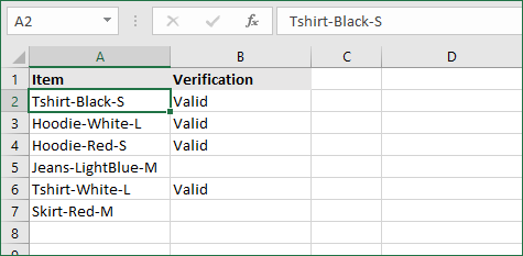
To extend the formula to more search terms, simply modify it by adding more strings using ISNUMBER(SEARCH(«string», cell)).
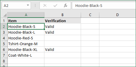
7. If cell contains several of many text strings, then return a value
This formula should be used if you’re looking to identify cells that contain several of the many words you’re searching for. For example, if you’re searching for two terms, the cell needs to contain both of them in order to be validated.
- Select the output cell, and use the following formula: =IF(AND(ISNUMBER(SEARCH(«string1»,cell)), ISNUMBER(SEARCH(«string2″,cell))), value_to_return,»»).
- For our example, the cell we want to check is A2. We’re looking for “hoodie” and “black”, and the return value will be Valid. In this scenario, you’d change the formula to =IF(AND(ISNUMBER(SEARCH(«hoodie»,A2)),ISNUMBER(SEARCH(«black»,A2))),»Valid «,»»).
- Because the A2 cell does contain both of the text values we searched for, the formula will return “Valid” to the output cell.
Final thoughts
We hope this article was useful to you in learning how to use “if cell contains” formulas in Microsoft Excel. Now, you can check if any cells contain values, text, numbers, and more. This allows you to navigate, manipulate and analyze your data efficiently.
We’re glad you’re read the article up to here  Thank you
You may also like
» How to use NPER Function in Excel
» How to Separate First and Last Name in Excel
» How to Calculate Break-Even Analysis in Excel
In this tutorial we’re going to explain how to use the Excel IF function (also known as IF Statement), and look at a couple of different applications for it.
With the IF statement you can tell Excel to perform different calculations depending on whether the answer to your question is true of false.
Watch the Video

Download Workbooks
Enter your email address below to download the sample workbook.
By submitting your email address you agree that we can email you our Excel newsletter.
IF Formula Builder
Our IF Formula Builder does the hard work of creating IF formulas.
You just need to enter a few pieces of information, and the workbook creates the formula for you.
Excel IF Function Written Tutorial
The function wizard in Excel describes the IF function as:
=IF(logical_test,value_if_true,value_if_false)
But let’s translate it into English and apply it to an example:
In the table below we want to calculate a commission in column G for each Builder based on the number of units in column D.

We’ll say that for units over 5 we’ll pay 10% commission based on the Total $k figure in column F, and for units of 5 and under we’ll pay 5% commission.
Our IF formula for row 2 would read like this:
=IF(The number of units in cell D2 is >5,Then take the Total $k in cell F2 x 10%, but if it’s not > 5 then take the Total $k in cell F2 x 5%)
The actual formula we would enter into Cell G2 would be:
=IF(D2>5,F2*10%,F2*5%)
Remember; as the number of units in row 5 is not greater than 5 the formula would calculate a 5% commission.
Other Uses for IF
We don’t have to use the IF function to perform a calculation. We could use it to return a comment. If we take the previous example again, we could have asked Excel to put a note in the cell like ‘Pay 5%’ or ‘Pay 10%’. To do this our IF formula would look like this:
=IF(D2>5,"Pay 10%","Pay 5%")
Notice the difference between the two formulas are the inverted commas («) surrounding the results we want Excel to produce. These inverted commas tell Excel that the information between them is to be entered as text.
Below is a screen shot of how the formula looks in the Formula Bar and the result returned in column G.
Try Other Operators
Because the IF formula is based on logic, you can employ tests other than the greater than (>) operator used in the example above.
Other operators you could use are:
| = | Equal to |
| < | Less Than |
| <= | Less than or equal to |
| >= | Greater than or equal to* |
| <> | Less than or greater than |
*If we’d used this operator in our above example row 5 which had 5 units would have returned Pay 10%.
The IF function runs a logical test and returns one value for a TRUE result, and another value for a FALSE result. The result from IF can be a value, a cell reference, or even another formula. By combining the IF function with other logical functions like AND and OR, you can test more than one condition at a time.
Syntax
The generic syntax for the IF function looks like this:
=IF(logical_test,[value_if_true],[value_if_false])The first argument, logical_test, is typically an expression that returns either TRUE or FALSE. The second argument, value_if_true, is the value to return when logical_test is TRUE. The last argument, value_if_false, is the value to return when logical_test is FALSE. Both value_if_true and value_if_false are optional, but you must provide one or the other. For example, if cell A1 contains 80, then:
=IF(A1>75,TRUE) // returns TRUE
=IF(A1>75,"OK") // returns "OK"
=IF(A1>85,"OK") // returns FALSE
=IF(A1>75,10,0) // returns 10
=IF(A1>85,10,0) // returns 0
=IF(A1>75,"Yes","No") // returns "Yes"
=IF(A1>85,"Yes","No") // returns "No"
Notice that text values like «OK», «Yes», «No», etc. must be enclosed in double quotes («»). However, numeric values should not be enclosed in quotes.
Logical tests
The IF function supports logical operators (>,<,<>,=) when creating logical tests. Most commonly, the logical_test in IF is a complete logical expression that will evaluate to TRUE or FALSE. The table below shows some common examples:
| Goal | Logical test |
|---|---|
| If A1 is greater than 75 | A1>75 |
| If A1 equals 100 | A1=100 |
| If A1 is less than or equal to 100 | A1<=100 |
| If A1 equals «Red» | A1=»red» |
| If A1 is not equal to «Red» | A1<>»red» |
| If A1 is less than B1 | A1<B1 |
| If A1 is empty | A1=»» |
| If A1 is not empty | A1<>»» |
| If A1 is less than current date | A1<TODAY() |
Notice text values must be enclosed in double quotes («»), but numbers do not. The IF function does not support wildcards, but you can combine IF with COUNTIF to get basic wildcard functionality. To test for substrings in a cell, you can use the IF function with the SEARCH function.
Pass or Fail example
In the worksheet shown above, we want to assign either «Pass» or «Fail» based on a test score. A passing score is 70 or higher. The formula in D6, copied down, is:
=IF(C5>=70,"Pass","Fail")
Translation: If the value in C5 is greater than or equal to 70, return «Pass». Otherwise, return «Fail».
Note that the logical flow of this formula can be reversed. This formula returns the same result:
=IF(C5<70,"Fail","Pass")
Translation: If the value in C5 is less than 70, return «Fail». Otherwise, return «Pass».
Both formulas above, when copied down, will return correct results.
Note: If you are new to the idea of formula criteria, this article explains many examples.
Assign points based on color
In the worksheet below, we want to assign points based on the color in column B. If the color is «red», the result should be 100. If the color is «blue», the result should be 125. This requires that we use a formula based on two IF functions, one nested inside the other. The formula in C5, copied down, is:
=IF(B5="red",100,IF(B5="blue",125))
Translation: IF the value in B5 is «red», return 100. Else, if the value in B5 is «blue», return 125.

There are three things to notice in this example:
- The formula will return FALSE if the value in B5 is anything except «red» or «blue»
- The text values «red» and «blue» must be enclosed in double quotes («»)
- The IF function is not case-sensitive and will match «red», «Red», «RED», or «rEd».
This is a simple example of a nested IFs formula. See below for a more complex example.
Return another formula
The IF function can return another formula as a result. For example, the formula below will return A1*5% when A1 is less than 100, and A1*7% when A1 is greater than or equal to 100:
=IF(A1<100,A1*5%,A1*7%)
Nested IF statements
The IF function can be «nested». A «nested IF» refers to a formula where at least one IF function is nested inside another in order to test for more conditions and return more possible results. Each IF statement needs to be carefully «nested» inside another so that the logic is correct. For example, the following formula can be used to assign a grade rather than a pass / fail result:
=IF(C6<70,"F",IF(C6<75,"D",IF(C6<85,"C",IF(C6<95,"B","A"))))
Up to 64 IF functions can be nested. However, in general, you should consider other functions, like VLOOKUP or XLOOKUP for more complex scenarios, because they can handle more conditions in a more streamlined fashion. For a more details see this article on nested IFs.
Note: the newer IFS function is designed to handle multiple conditions without nesting. However, a lookup function like VLOOKUP or XLOOKUP is usually a better approach unless the logic for each condition is custom.
IF with AND, OR, NOT
The IF function can be combined with the AND function and the OR function. For example, to return «OK» when A1 is between 7 and 10, you can use a formula like this:
=IF(AND(A1>7,A1<10),"OK","")
Translation: if A1 is greater than 7 and less than 10, return «OK». Otherwise, return nothing («»).
To return B1+10 when A1 is «red» or «blue» you can use the OR function like this:
=IF(OR(A1="red",A1="blue"),B1+10,B1)
Translation: if A1 is red or blue, return B1+10, otherwise return B1.
=IF(NOT(A1="red"),B1+10,B1)
Translation: if A1 is NOT red, return B1+10, otherwise return B1.
IF cell contains specific text
Because the IF function does not support wildcards, it is not obvious how to configure IF to check for a specific substring in a cell. A common approach is to combine the ISNUMBER function and the SEARCH function to create a logical test like this:
=ISNUMBER(SEARCH(substring,A1)) // returns TRUE or FALSEFor example, to check for the substring «xyz» in cell A1, you can use a formula like this:
=IF(ISNUMBER(SEARCH("xyz",A1)),"Yes","No")Read a detailed explanation here.
More information
- Read more about nested IFs
- Learn how to use VLOOKUP instead of nested IFs (video)
- 50 Examples of formula criteria
Notes
- The IF function is not case-sensitive.
- To count values conditionally, use the COUNTIF or the COUNTIFS functions.
- To sum values conditionally, use the SUMIF or the SUMIFS functions.
- If any of the arguments to IF are supplied as arrays, the IF function will evaluate every element of the array.