
Excel for Microsoft 365 Excel 2021 Excel 2019 Excel 2016 Excel 2013 Excel 2010 Excel 2007 More…Less
To select all cells on a worksheet, use one of the following methods:
-
Click the Select All button.

-
Press CTRL+A.
Note If the worksheet contains data, and the active cell is above or to the right of the data, pressing CTRL+A selects the current region. Pressing CTRL+A a second time selects the entire worksheet.
Tip If you want to select all cells in the active range, press CTRL+SHIFT+*.
Need more help?
Содержание
- Select cell contents in Excel
- Select one or more cells
- Select one or more rows and columns
- Select table, list or worksheet
- Need more help?
- Find and select cells that meet specific conditions
- Need more help?
- 7 Easy Ways to Select Multiple Cells in Excel
- Select Multiple Cells (that are all contiguous)
- Select Rows/Columns
- Select a Single Row/Column
- Select Multiple Rows/Columns
- Select Multiple Non-Adjacent Rows/Columns
- Select All the Cells in the Current Table/Data
- Select All the Cells in the Worksheet
- Select Multiple Non-Contiguous Cells
- Select Cells Using Name Box
- Select a Named Range
Select cell contents in Excel
In Excel, you can select cell contents of one or more cells, rows and columns.

Note: If a worksheet has been protected, you might not be able to select cells or their contents on a worksheet.
Select one or more cells
Click on a cell to select it. Or use the keyboard to navigate to it and select it.
To select a range, select a cell, then with the left mouse button pressed, drag over the other cells.
Or use the Shift + arrow keys to select the range.
To select non-adjacent cells and cell ranges, hold Ctrl and select the cells.
Select one or more rows and columns
Select the letter at the top to select the entire column. Or click on any cell in the column and then press Ctrl + Space.
Select the row number to select the entire row. Or click on any cell in the row and then press Shift + Space.
To select non-adjacent rows or columns, hold Ctrl and select the row or column numbers.
Select table, list or worksheet
To select a list or table, select a cell in the list or table and press Ctrl + A.
To select the entire worksheet, click the Select All button at the top left corner.

Note: In some cases, selecting a cell may result in the selection of multiple adjacent cells as well. For tips on how to resolve this issue, see this post How do I stop Excel from highlighting two cells at once? in the community.
Click the cell, or press the arrow keys to move to the cell.
A range of cells
Click the first cell in the range, and then drag to the last cell, or hold down SHIFT while you press the arrow keys to extend the selection.
You can also select the first cell in the range, and then press F8 to extend the selection by using the arrow keys. To stop extending the selection, press F8 again.
A large range of cells
Click the first cell in the range, and then hold down SHIFT while you click the last cell in the range. You can scroll to make the last cell visible.
All cells on a worksheet
Click the Select All button.
To select the entire worksheet, you can also press CTRL+A.
Note: If the worksheet contains data, CTRL+A selects the current region. Pressing CTRL+A a second time selects the entire worksheet.
Nonadjacent cells or cell ranges
Select the first cell or range of cells, and then hold down CTRL while you select the other cells or ranges.
You can also select the first cell or range of cells, and then press SHIFT+F8 to add another nonadjacent cell or range to the selection. To stop adding cells or ranges to the selection, press SHIFT+F8 again.
Note: You cannot cancel the selection of a cell or range of cells in a nonadjacent selection without canceling the entire selection.
An entire row or column
Click the row or column heading.
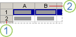
2. Column heading
You can also select cells in a row or column by selecting the first cell and then pressing CTRL+SHIFT+ARROW key (RIGHT ARROW or LEFT ARROW for rows, UP ARROW or DOWN ARROW for columns).
Note: If the row or column contains data, CTRL+SHIFT+ARROW key selects the row or column to the last used cell. Pressing CTRL+SHIFT+ARROW key a second time selects the entire row or column.
Adjacent rows or columns
Drag across the row or column headings. Or select the first row or column; then hold down SHIFT while you select the last row or column.
Nonadjacent rows or columns
Click the column or row heading of the first row or column in your selection; then hold down CTRL while you click the column or row headings of other rows or columns that you want to add to the selection.
The first or last cell in a row or column
Select a cell in the row or column, and then press CTRL+ARROW key (RIGHT ARROW or LEFT ARROW for rows, UP ARROW or DOWN ARROW for columns).
The first or last cell on a worksheet or in a Microsoft Office Excel table
Press CTRL+HOME to select the first cell on the worksheet or in an Excel list.
Press CTRL+END to select the last cell on the worksheet or in an Excel list that contains data or formatting.
Cells to the last used cell on the worksheet (lower-right corner)
Select the first cell, and then press CTRL+SHIFT+END to extend the selection of cells to the last used cell on the worksheet (lower-right corner).
Cells to the beginning of the worksheet
Select the first cell, and then press CTRL+SHIFT+HOME to extend the selection of cells to the beginning of the worksheet.
More or fewer cells than the active selection
Hold down SHIFT while you click the last cell that you want to include in the new selection. The rectangular range between the active cell and the cell that you click becomes the new selection.
Need more help?
You can always ask an expert in the Excel Tech Community or get support in the Answers community.
Источник
Find and select cells that meet specific conditions
Use the Go To command to quickly find and select all cells that contain specific types of data, such as formulas. Also, use Go To to find only the cells that meet specific criteria,—such as the last cell on the worksheet that contains data or formatting.
Follow these steps:
Begin by doing either of the following:
To search the entire worksheet for specific cells, click any cell.
To search for specific cells within a defined area, select the range, rows, or columns that you want. For more information, see Select cells, ranges, rows, or columns on a worksheet.
Tip: To cancel a selection of cells, click any cell on the worksheet.
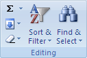
On the Home tab, click Find & Select > Go To (in the Editing group).
Keyboard shortcut: Press CTRL+G.
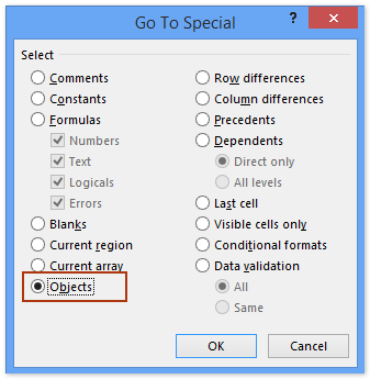
In the Go To Special dialog box, click one of the following options.
Cells that contain comments.
Cells that contain constants.
Cells that contain formulas.
Note: The check boxes below Formulas define the type of formula.
The current region, such as an entire list.
An entire array if the active cell is contained in an array.
Graphical objects, including charts and buttons, on the worksheet and in text boxes.
All cells that differ from the active cell in a selected row. There is always one active cell in a selection—whether this is a range, row, or column. By pressing the Enter or Tab key, you can change the location of the active cell, which by default is the first cell in a row.
If more than one row is selected, the comparison is done for each individual row of that selection, and the cell that is used in the comparison for each additional row is located in the same column as the active cell.
All cells that differ from the active cell in a selected column. There is always one active cell in a selection, whether this is a range, row, or column. By pressing the Enter or Tab key, you can change the location of the active cell—which by default is the first cell in a column.
When selecting more than one column, the comparison is done for each individual column of that selection. The cell that is used in the comparison for each additional column is located in the same row as the active cell.
Cells that are referenced by the formula in the active cell. Under Dependents, do either of the following:
Click Direct only to find only cells that are directly referenced by formulas.
Click All levels to find all cells that are directly or indirectly referenced by the cells in the selection.
Cells with formulas that refer to the active cell. Do either of the following:
Click Direct only to find only cells with formulas that refer directly to the active cell.
Click All levels to find all cells that directly or indirectly refer to the active cell.
The last cell on the worksheet that contains data or formatting.
Visible cells only
Only cells that are visible in a range that crosses hidden rows or columns.
Only cells that have conditional formats applied. Under Data validation, do either of the following:
Click All to find all cells that have conditional formats applied.
Click Same to find cells that have the same conditional formats as the currently selected cell.
Only cells that have data validation rules applied. Do either of the following:
Click All to find all cells that have data validation applied.
Click Same to find cells that have the same data validation as the currently selected cell.
Need more help?
You can always ask an expert in the Excel Tech Community or get support in the Answers community.
Источник
7 Easy Ways to Select Multiple Cells in Excel
Selecting a cell is one of the most basic things users do in Excel.
There are many different ways to select a cell in Excel – such as using the mouse or the keyboard (or a combination of both).
In this article, I would show you how to select multiple cells in Excel. These cells could all be together (contiguous) or separated (non-contiguous)
While this is quite simple, I’m sure you’ll pick up a couple of new tricks to help you speed up your work and be more efficient.
So let’s get started!
This Tutorial Covers:
Select Multiple Cells (that are all contiguous)
If you know how to select one cell in Excel, I’m sure you also know how to select multiple cells.
But let me still cover this anyway.
Suppose you want to select cells A1:D10.
Below are the steps to do this:
- Place the cursor on cell A1
- Select cell A1 (by using the left mouse button). Keep the mouse button pressed.
- Drag the cursor till cell D10 (so that it covers all the cells between A1 and D10)
- Leave the mouse button

Now let’s see some more cases.
Select Rows/Columns
A lot of times, you will be required to select an entire row or column (or even multiple rows or columns). These could be to hide or delete these rows/columns, move it around in the worksheet, highlight it, etc.
Just like you can select a cell in Excel by placing the cursor and clicking the mouse, you can also select a row or a column by simply clicking on the row number or column alphabet.
Let’s go through each of these cases.
Select a Single Row/Column
Here is how you can select an entire row in Excel:
- Bring the cursor over the row number of the row that you want to select
- Use the left mouse-click to select the entire row


When you select the entire row, you will see that the color of that selection changes (it becomes a bit darker as compared to the rest of the cell in the worksheet).
Just like we have selected a row in Excel, you can also select a column (where instead of clicking on the row number, you have to click on the column alphabet, which is at the top of the column).
Select Multiple Rows/Columns
Now, what if you don’t want to select just one row.
What if you want to select multiple rows?
For example, let’s say that you want to select row number 2, 3, and 4 at the same time.
Here is how to do that:
- Place the cursor over row number 2 in the worksheet
- Press the mouse left button while your cursor is on row number two (keep the mouse button pressed)
- Keep the mouse left-button still pressed and drag the cursor down till row 4
- Leave the mouse button

You’ll see that this would select three adjacent rows that you covered through your mouse.
Just like we have selected three adjacent rows, you can follow the same steps to select multiple columns as well.
Select Multiple Non-Adjacent Rows/Columns
What if you want to select multiple rows, but these are not-adjacent.
For example, you may want to select row numbers 2, 4, 7.
In such a case you cannot use the mouse drag technique covered above because it would select all the rows in between.
To do this, you will have to use a combination of keyboard and mouse.
Here is how to select non-adjacent multiple rows in Excel:
- Place the cursor over row number 2 in the worksheet
- Hold the Control key on your keyboard
- Press the mouse left button while your cursor is on row number 2
- Leave the mouse button
- Place the cursor over the next row you want to select (row 4 in this case),
- Hold the Control key on your keyboard
- Press the mouse left button while your cursor is on row number 4. Once row 4 is also selected, leave the mouse button
- Repeat the same to select row 7 as well
- Leave the Control key

The above steps would select multiple non-adjacent rows in the worksheet.
You can use the same method to select multiple non-adjacent columns.
Select All the Cells in the Current Table/Data
Most of the time, when you have to select multiple cells in Excel, these would be the cells in a specific table or a dataset.
You can do this by using a simple keyboard shortcut.
Below are the steps to select all the cells in the current table:
- Select any cell within the data set
- Hold the Ctrl key and then press the A key


The above steps would select all the cells in the data set (where Excel considers this data set to extend until it encounters a blank row or column).
As soon as Excel encounters a blank row or blank column, it would consider this as the end of the data set (so anything beyond the blank row/column will not be selected)
Select All the Cells in the Worksheet
Another common task that is often done is to select all the cells in the worksheet.
I often work with data downloaded from different databases, and often this data is formatted in a certain way. And my first step as soon as I get this data is to select all the cells and remove all the formatting.
Here is how you can select all the cells in the active worksheet:
- Select the worksheet in which you want to select all the cells
- Click on the small inverted triangle at the top left part of the worksheet

This would instantly select all the cells in the entire worksheet (note that this would not select any object such as a chart or shape in the worksheet).
And if you are a keyboard shortcut aficionado, you can use the below shortcut:
If you have selected a blank cell that does not have any data around it, you don’t need to press the A key twice (just use Control-A).
Select Multiple Non-Contiguous Cells
The more you work with Excel, the more you would have a need to select multiple non-contiguous cells (such as A2, A4, A7, etc.)
Below I have an example where I only want to select the records for the US. And since these are not adjacent to each other, I somehow need to figure out how to select all these multiple cells at the same time.

Again, you can do this easily using a combination of keyboard and mouse.
Below are the steps to do this:
- Hold the Control key on the keyboard
- One by one, select all the non-contiguous cells (or range of cells) that you want to remain selected
- When done, leave the Control key

The above technique also works when you want to select non-contiguous rows or columns. You can simply hold the Control key and select the non-adjacent rows/columns.
Select Cells Using Name Box
So far we have seen examples where we could manually select the cells because they were close by.
But in some cases, you may have to select multiple cells or rows/columns that are far off in the worksheet.
Of course, you can do that manually, but you’ll soon realize that it’s time-consuming and error-prone.
If it’s something you have to do quite often (that is, select the same cells or rows/columns), you can use the Name Box to do it a lot faster.
Name Box is the small field that you have on the left of the formula bar in Excel.

When you type a cell reference (or a range reference) in the name box, it selects all the specified cells.
For example, let’s say I want to select cell A1, K3, and M20
Since these are quite far off, if I try and select these using the mouse, I would have to scroll a little bit.
This may be justified if you only have to do it once in a while, but in case you have to say select the same cells often, you can use the name box instead.
Below are the steps to select multiple cells using the name box:
- Click on the name box
- Enter the cell references that you want to select (separated by comma)
- Hit the enter key

The above steps would instantly select all the cells that you have entered in the name box.
Of these selected cells, one would be the active cell (and the cell reference of the active cell would now be visible in the name box).
Select a Named Range
If you have created a named range in Excel, you can also use the Name Box to refer to the entire named range (instead of using the cell references as shown in the method above)
If you don’t know what a Named Range is, it’s when you assign a name to a cell or a range of cells and then use the name instead of the cell reference in formulas.
Below are the steps to quickly create a Named Range in Excel:
- Select the cells that you want to be included in the Named Range
- Click on the Name box (which is the field adjacent to the formula bar)
- Enter the name that you want to assign to the selected range of cells (you can’t have spaces in the name)
- Hit the Enter key

The above steps would create a Named Range for the cells that you selected.
Now, if you want to quickly select these same cells, instead of doing that manually you can simply go to the Name box and enter the name of the named range (or click on the dropdown icon and select the name from there)

This would instantly select all the cells that are part of that Named Range.
So, these are some of the methods that you can use to select multiple cells in Excel.
I hope you found this tutorial useful.
Other Excel tutorials you may like:
Источник
Click the Select All button. Press CTRL+A. Note If the worksheet contains data, and the active cell is above or to the right of the data, pressing CTRL+A selects the current region. Pressing CTRL+A a second time selects the entire worksheet.
Contents
- 1 What is the fastest way to select all data in Excel?
- 2 How do I quickly select thousands of rows in Excel?
- 3 How do I select all data in a column?
- 4 How do I select all below in Excel?
- 5 How do I select all cells to the right in Excel?
- 6 How do you select all in Excel without dragging?
- 7 How do I select 5000 rows in Excel?
- 8 How do I select all without scrolling?
- 9 How do you select a whole column in Excel?
- 10 How do I select all below?
- 11 How do I select all text in an Excel cell?
- 12 How do you select all cells with data in a column Excel?
- 13 How do you select a large range of cells in Excel without scrolling?
- 14 How do I copy data from all cells in Excel?
- 15 How do you select multiple cells in Excel without rows?
- 16 How do I select 500 cells in Excel?
- 17 How do I delete 1000 rows in Excel?
- 18 How do I select multiple cells in Excel without a mouse?
What is the fastest way to select all data in Excel?
Select All Cells. Press Ctrl + A a second time to select all cells on the sheet. If your spreadsheet has multiple blocks of data, Excel does a pretty good job of selecting the block of data that is surrounding your cell when you press Ctrl + A .
How do I quickly select thousands of rows in Excel?
Select Multiple Entire Rows of Cells.
Continuing to hold down your mouse button, drag your cursor across all the rows you want to select. Or, if you prefer, you can hold down your Shift key and click the bottom-most row you want to select.
How do I select all data in a column?
Ctrl + Space is the keyboard is the shortcut to select an entire column. Select the column header and press Shift + End + ↓ (Down Arrow) to select that column. Ctrl + Space is the keyboard is the shortcut to select an entire column.
How do I select all below in Excel?
Click on the top cell, then press Ctrl and hold the space bar. All cells beneath the cell initially chosen will be highlighted.
How do I select all cells to the right in Excel?
If we’d like to select all the cells to the right within a data region, we simply hold Control + Shift and press the right arrow key. If we now press Control + Shift and the down arrow key, it selects the whole region.
How do you select all in Excel without dragging?
To select a range of cells without dragging the mouse:
- Click in the cell which is to be one corner of the range of cells.
- Move the mouse to the opposite corner of the range of cells.
- Hold down the Shift key and click.
How do I select 5000 rows in Excel?
Select one or more rows and columns
- Select the letter at the top to select the entire column. Or click on any cell in the column and then press Ctrl + Space.
- Select the row number to select the entire row.
- To select non-adjacent rows or columns, hold Ctrl and select the row or column numbers.
How do I select all without scrolling?
“Easily select all the way down without the mouse/scrolling”
By default you can start this tool with the shortcut Control+Alt+L.
How do you select a whole column in Excel?
Select any cell in any column. Press Ctrl + Space shortcut keys on the keyboard. The whole column will be highlighted in excel to show the selected column, as shown below in the picture. You can also say that this is a shortcut to highlight column in excel.
How do I select all below?
Click to put the cursor on where you want to select everything below, the press the Ctrl + Shift + End keys at the same time. Then all contents after the cursor are selected immediately.
How do I select all text in an Excel cell?
Selecting Cells that contain specific Text
- #1 go to HOME tab, click Find & Select command under Editing group. And the Find and Replace dialog will open.
- #2 type one text string that you want to find in your data.
- #3 click Find All button.
- #4 press Ctrl +A keys in your keyboard to select all searched values.
How do you select all cells with data in a column Excel?
You can also click anywhere in the table column, and then press CTRL+SPACEBAR, or you can click the first cell in the table column, and then press CTRL+SHIFT+DOWN ARROW. Note: Pressing CTRL+SPACEBAR once selects the table column data; pressing CTRL+SPACEBAR twice selects the entire table column.
How do you select a large range of cells in Excel without scrolling?
You can do this two ways:
- Click into the cell in the upper left corner of the range.
- Click into the Name Box and type the cell in the lower right corner of the range.
- Press SHIFT + Enter.
- Excel will select the entire range.
How do I copy data from all cells in Excel?
Select the cell or range of cells. Select Copy or press Ctrl + C. Select Paste or press Ctrl + V.
Copy cell values, cell formats, or formulas only
- To paste values only, click Values.
- To paste cell formats only, click Formatting.
- To paste formulas only, click Formulas.
How do you select multiple cells in Excel without rows?
Just press and hold down the Ctrl key, and you can select multiple non-adjacent cells or ranges with mouse clicking or dragging in active worksheet. This does not require holding down keys during selection.
How do I select 500 cells in Excel?
Here are the steps to select 500 cells in one go:
- Click in the Name Box.
- Type A1:A500.
- Hit Enter.
How do I delete 1000 rows in Excel?
How can I delete multiple rows in Excel?
- Open the Excel sheet and select all the rows that you want to delete.
- Right-click the selection and click Delete or Delete rows from the list of options.
- Alternatively, click the Home tab, navigate to the Cells group, and click Delete.
- A drop-down menu will open on your screen.
How do I select multiple cells in Excel without a mouse?
No Mouse Needed
Start by selecting cell B4. To select the first block of data, hold down Ctrl+Shift and press the down arrow (↓) and then the right arrow (→). This common keyboard trick selects all the way down to the bottom and the right edge of the data.
In this article you’ll learn all of the different Select All shortcuts in Word, Excel and PowerPoint, and how to use Select All to quickly grab things like:
- Objects (PowerPoint)
- Text with similar formatting (Word)
- Formulas (Excel)
- Constants (Excel)
- Comments (Excel)
- And more!
This allows you to quickly grab EXACTLY what you need in each of the programs when you need it. This saves you from otherwise having to manually selecting everything yourself, one-by-one.
Select All shortcut (A Must Know)
The universal Select All shortcut for most program (Mac or PC) is:

Select All shortcut (PC Users): Ctrl + A
Select All shortcut (Mac Users) Cmd + A
That said there are a variety of different ways you can use the shortcut in Word, Excel and PowerPoint to finish your tasks faster and get you to Happy Hour (all discussed below).
How to best use the Select All command?
In short, this command is best used to quickly grab all the text, numbers, objects, formulas etc. that you want to quickly format or work with.
This allows you to quickly make changes to everything at once. For example:
- Change the font style of all the text in a Word document
- Grab all the formulas or constants in an Excel spreadsheet to change their font color
- Grab all your PowerPoint objects on a slide to change their shape fill
Which makes sense, right?
Why bother doing things manually (one-by-one) when you can select all your objects at once.
And it’s this kind of know-how why one person leaves the office at a decent hour, while another wastes away at the office all night.
How to Select All in Word

You have 4 different types of selection options in Microsoft Word.
And if you are on a PC, you can additionally shortcut all of these using your Ribbon Guides (details below).

1. Select All (Ctrl + A)
Selects everything within your document so that you can make all the formatting edits that you want at the same time.
Clicking this command with your mouse is the same as hitting Ctrl + A on your keyboard (Cmd + A on a Mac).
2. Select Objects
Changes your mouse cursor into an arrow symbol that allows you to select an element (chart, picture, SmartArt graphic, etc.) as an object.
This is different than when you click things with your mouse. When you click with your mouse, you normally click into the object as if you are going to edit it.
The Select Objects command ensures that you select the object itself. That way you can cut and paste it, or move it around within your document.
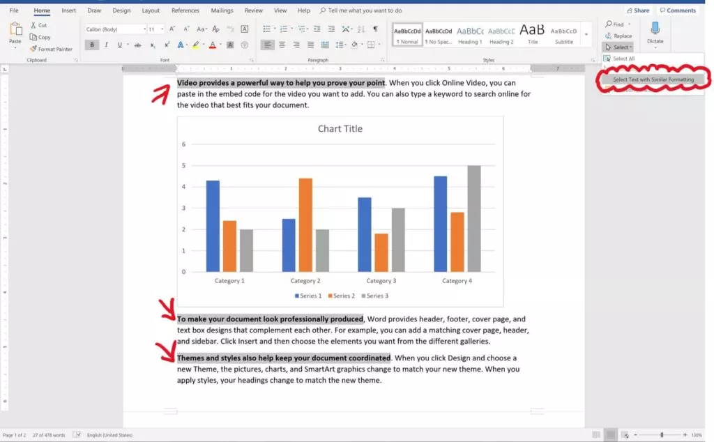
3. Select Text with Similar Formatting
Selects all of the text within a Word document that matches the formatting of the text that you have already selected.
This is one of the coolest features in Microsoft Word that hardly anyone knows about. This command grabs all of the same formatted text within a document, so you can change it’s formatting all at once.
Ahem… amazing!
4. The Selection Pane in Word (Alt + F10)
Opens or closes the Selection Pane in Microsoft Word.
Inside the Selection Pane you can see (and quickly manipulate) all the objects in a Word document.
Similar to the Selection Pane in PowerPoint, it only only shows you the objects on the current page you are currently working on.
That means that if you have 100 charts in your Word document but only 1 chart on your current page, you will only see 1 chart in the Selection Pane.
Select All Shortcuts in Word (Ribbon Guides)
Instead of using your mouse to access the selection commands, on a PC you can use your Ribbon Guides.
To use these shortcuts, simply hit the Alt key on your keyboard. Hitting the Alt key, you will see alphabetical sequences to the commands across your Ribbon.

On a PC, your select all Ribbon Guide shortcuts are:
- Select All: Alt, H, SL, A
- Select Objects: Alt, H, SL, O
- Select Text with Similar Formatting: Alt, H, SL, S
- Selection Pane: Alt, H, SL, P
Note: When using your Ribbon Guide shortcuts in Word, you do not need to hold them down. Instead, simply hit and let go of them one at a time (following the letters forward).
To learn more about the Microsoft Office ribbon, see this guide by Microsoft here.
Select All in Excel
Because there are so many more inputs that can go into an Excel spreadsheet, there are 7 different selection commands in Excel (all covered below)
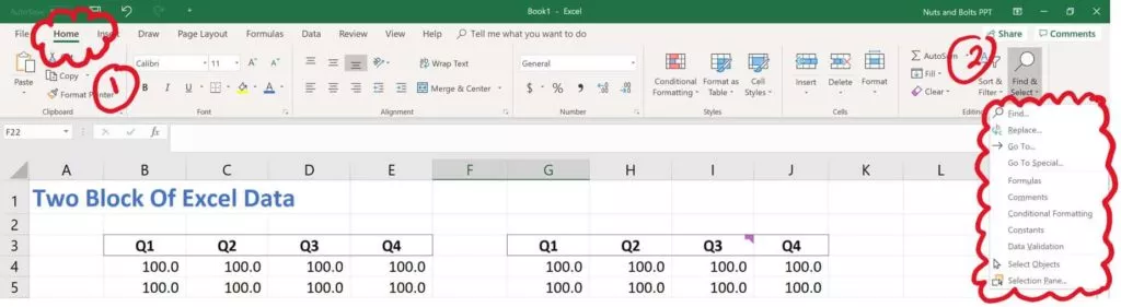
1. Select All (Ctrl + A)
Hitting Ctrl + A triggers the Select All command (which is otherwise not up in your Excel ribbon.
It’s also important to note that the Select All command works a little bit differently in Excel.
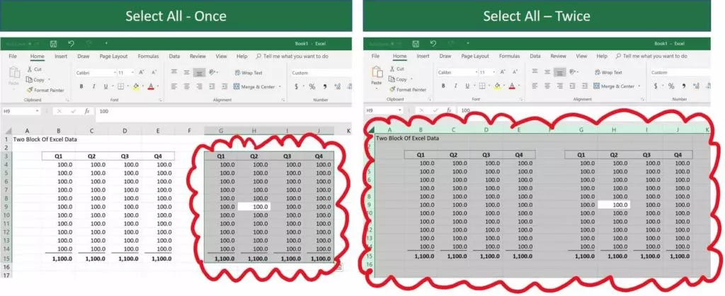
Using the command once, first selects the block of cells that you are currently active in.
Using the command a second time, then selects everything within your spreadsheet.
See images above for hitting it once, then twice.
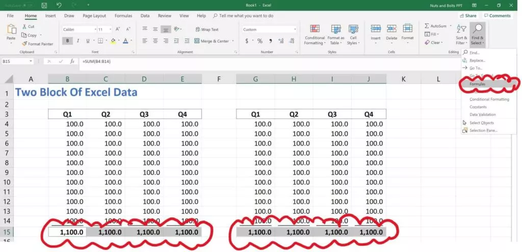
2. Select Formulas
Clicking Formulas will grab all the formulas in your current spreadsheet (pictured below).
This is a fast way and easy way to quickly identify and change the formatting of any formulas in your spreadsheet.
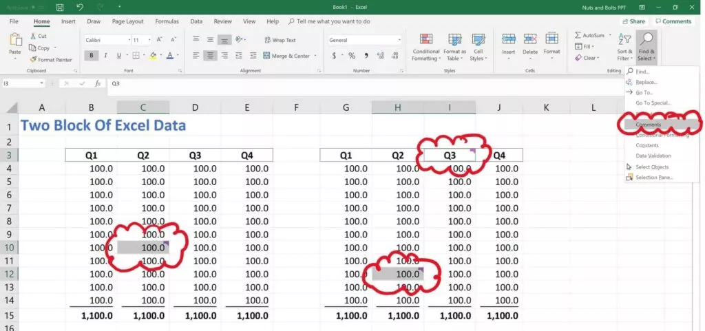
3. Select Comments
Clicking Comments automatically selects all of the comments in your spreadsheet (pictured below).
Comments show up in your spreadsheet as little markers in the upper-right hand corner of your cells. If you don’t want to waste time searching for them, simply use these command.
This allows you to quickly grab all the comments in your spreadsheet and format the cells.
4. Select Conditional Formatting
Clicking Conditional Formatting selects any cells within your spreadsheet that have conditional formatting in them.
This allows you to spot check or change the conditional formatting rules for those specific cells.
To learn more about conditional formatting rules, and how to use them, see this article by Microsoft here.
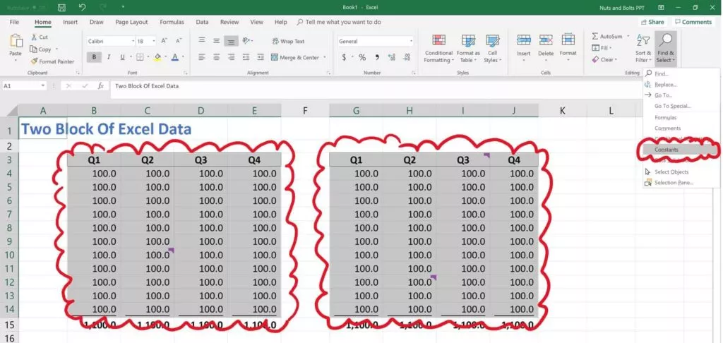
5. Select Constants
Selects all the constant values in your spreadsheet (i.e. values that are not formula-driven).
This is a fast and easy way to find all of the inputs that someone is using in their financial model or spreadsheet so that you can double-check their assumptions (pictured below).
6. Select Objects
Turns your cursor into an arrow that allows you to select objects that are within your spreadsheet (charts, pictures, SmartArt graphics etc.).
This is useful when you have a large spreadsheet or dashboard and you want to just select a single graphic without accidentally selecting the cells around it.
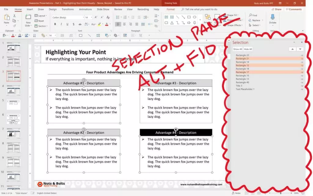
7. The Selection Pane in Excel (Alt + F10)
Opens the Selection Pane in Excel, showing you all of the charts, pictures, SmartArt graphics, etc., that are currently within your active spreadsheet.
Just keep in mind that the Selection Pane will only show you objects that are within the current sheet you are on. It will not show you objects that are on other sheets within your Excel file.
Select All Shortcuts in Excel (Ribbon Guides):
On top of using your mouse to activate the different Select commands in Excel, if you are on a PC, you can also use your Ribbon Guides to shortcut these commands (see key combinations below).
If you use any of these selection commands A LOT when working in Excel and are on a PC, I highly recommend learning these key combinations to save you time.

On a PC, your Ribbon Guide Shortcuts to these different commands are:
- Formulas: Alt, H, FD, U
- Comments: Alt, H, FD, M
- Conditional Formatting: Alt, H, FD, C
- Constants: Alt, H, FD, N
- Data Validation: Alt, H, FD, V
- Select Objects: Alt, H, FD, O
- Selection Pane: Alt, H, FD, P
Note: When using your Ribbon Guide shortcuts, you do not need to hold down the keys to make them work. Instead, simply hit and let go of them one at a time.
Select All in PowerPoint

You have 3 different types of selection options in PowerPoint (all of which you can shortcut on a PC using your Ribbon Guide shortcuts as discussed further below).

1. Select All (Ctrl + A)
Selects all of the objects that are currently on your slide.
This shortcut works in all of the different PowerPoint views including:
- The Normal View
- The Slide Master View
- The Handout Master View
- The Notes Master View, etc.
To learn more about setting up these different views in PowerPoint, see our guide on custom PowerPoint templates here.
On top of that, if you first click into the thumbnail view (pictured below) you can use the command to grab all of your slides. This allows you to copy and paste those slides, apply a new layout, reset the slides, etc.
2. Select Objects
This is the default selection option in PowerPoint, allowing you to select objects (shapes, text boxes, charts, SmartArt graphics, etc.) which is what all of your slides are made of.
3. Selection Pane in PowerPoint (Alt + F10)
Opens the Selection Pane in PowerPoint, giving you a bird’s eye view of everything that is on your slide (even if it is buried beneath something else).
To learn other useful PowerPoint shortcuts like this to save you time in the program, see our guide here.
Selection Pane Shortcuts in PowerPoint
To learn more about how to use the Selection Pane shortcuts in PowerPoint, watch the short video below.
Inverse selected objects in PowerPoint
Another way to cleverly use the Select All command in PowerPoint is to ‘inverse-select’ your objects.
For example, let’s say you want to select EVERYTHING on your slide except for the title.
To do so, follow these steps:
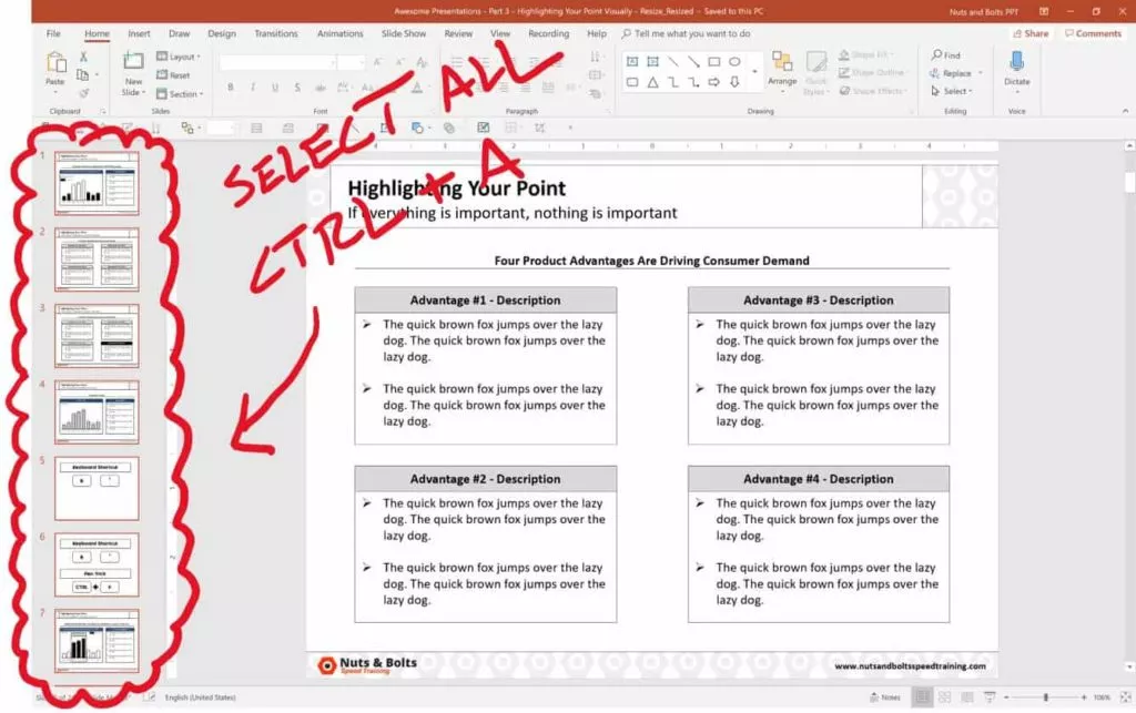
- Hit Ctrl + A to select everything on your slide
- While holding the Shift key or the Ctrl key, select your Title to un-select it
Doing so leaves you with everything on your slide selected except for your slide title (or whatever else you unselected by holding the Shift or Ctrl key).
Select All shortcuts in PowerPoint (Ribbon Guides)
Besides navigating these selection commands using your mouse, you can also use your Ribbon Guide shortcuts to access them if you are on a PC.
To use your Ribbon Guide shortcuts, simply hit and let go of the Alt key, and then follow the alphabetical or numerical queues to find your command (all shortcut combinations are listed below).

On a PC, your Select All Ribbon Shortcuts are:
- Select All: Alt, H, SL, A
- Select Objects: Alt, H, SL, O
- Selection Pane: Alt, H, SL, P
Note: When using your Ribbon Guide shortcuts, you do not need to hold down the keys to make them work. Instead, simply hit and let go of them one at a time.
Conclusion
So those all the different ways you can Select All in Word, Excel and PowerPoint, and the different Select All shortcuts available to you if you are on a PC version of Microsoft Office.
Knowing how to properly use these, allows you to quickly grab exactly what you’re looking for so you can format it. This saves you time and gets you once step closer to Happy Hour.
If you are interested in taking your PowerPoint skills to the next level, you can learn more about our online courses and training here.
What’s next?
Selecting a cell is one of the most basic things users do in Excel.
There are many different ways to select a cell in Excel – such as using the mouse or the keyboard (or a combination of both).
In this article, I would show you how to select multiple cells in Excel. These cells could all be together (contiguous) or separated (non-contiguous)
While this is quite simple, I’m sure you’ll pick up a couple of new tricks to help you speed up your work and be more efficient.
So let’s get started!
Select Multiple Cells (that are all contiguous)
If you know how to select one cell in Excel, I’m sure you also know how to select multiple cells.
But let me still cover this anyway.
Suppose you want to select cells A1:D10.
Below are the steps to do this:
- Place the cursor on cell A1
- Select cell A1 (by using the left mouse button). Keep the mouse button pressed.
- Drag the cursor till cell D10 (so that it covers all the cells between A1 and D10)
- Leave the mouse button
Easy-peasy, right?
Now let’s see some more cases.
Select Rows/Columns
A lot of times, you will be required to select an entire row or column (or even multiple rows or columns). These could be to hide or delete these rows/columns, move it around in the worksheet, highlight it, etc.
Just like you can select a cell in Excel by placing the cursor and clicking the mouse, you can also select a row or a column by simply clicking on the row number or column alphabet.
Let’s go through each of these cases.
Select a Single Row/Column
Here is how you can select an entire row in Excel:
- Bring the cursor over the row number of the row that you want to select

- Use the left mouse-click to select the entire row

When you select the entire row, you will see that the color of that selection changes (it becomes a bit darker as compared to the rest of the cell in the worksheet).
Just like we have selected a row in Excel, you can also select a column (where instead of clicking on the row number, you have to click on the column alphabet, which is at the top of the column).
Also read: Select Till End of Data in a Column in Excel (Shortcuts)
Select Multiple Rows/Columns
Now, what if you don’t want to select just one row.
What if you want to select multiple rows?
For example, let’s say that you want to select row number 2, 3, and 4 at the same time.
Here is how to do that:
- Place the cursor over row number 2 in the worksheet
- Press the mouse left button while your cursor is on row number two (keep the mouse button pressed)
- Keep the mouse left-button still pressed and drag the cursor down till row 4
- Leave the mouse button
You’ll see that this would select three adjacent rows that you covered through your mouse.
Just like we have selected three adjacent rows, you can follow the same steps to select multiple columns as well.
Select Multiple Non-Adjacent Rows/Columns
What if you want to select multiple rows, but these are not-adjacent.
For example, you may want to select row numbers 2, 4, 7.
In such a case you cannot use the mouse drag technique covered above because it would select all the rows in between.
To do this, you will have to use a combination of keyboard and mouse.
Here is how to select non-adjacent multiple rows in Excel:
- Place the cursor over row number 2 in the worksheet
- Hold the Control key on your keyboard
- Press the mouse left button while your cursor is on row number 2
- Leave the mouse button
- Place the cursor over the next row you want to select (row 4 in this case),
- Hold the Control key on your keyboard
- Press the mouse left button while your cursor is on row number 4. Once row 4 is also selected, leave the mouse button
- Repeat the same to select row 7 as well
- Leave the Control key
The above steps would select multiple non-adjacent rows in the worksheet.
You can use the same method to select multiple non-adjacent columns.
Select All the Cells in the Current Table/Data
Most of the time, when you have to select multiple cells in Excel, these would be the cells in a specific table or a dataset.
You can do this by using a simple keyboard shortcut.
Below are the steps to select all the cells in the current table:
- Select any cell within the data set

- Hold the Ctrl key and then press the A key

The above steps would select all the cells in the data set (where Excel considers this data set to extend until it encounters a blank row or column).
As soon as Excel encounters a blank row or blank column, it would consider this as the end of the data set (so anything beyond the blank row/column will not be selected)
Select All the Cells in the Worksheet
Another common task that is often done is to select all the cells in the worksheet.
I often work with data downloaded from different databases, and often this data is formatted in a certain way. And my first step as soon as I get this data is to select all the cells and remove all the formatting.
Here is how you can select all the cells in the active worksheet:
- Select the worksheet in which you want to select all the cells
- Click on the small inverted triangle at the top left part of the worksheet

This would instantly select all the cells in the entire worksheet (note that this would not select any object such as a chart or shape in the worksheet).
And if you are a keyboard shortcut aficionado, you can use the below shortcut:
Control + A + A (hold the control key and press the A key twice)
If you have selected a blank cell that does not have any data around it, you don’t need to press the A key twice (just use Control-A).
Select Multiple Non-Contiguous Cells
The more you work with Excel, the more you would have a need to select multiple non-contiguous cells (such as A2, A4, A7, etc.)
Below I have an example where I only want to select the records for the US. And since these are not adjacent to each other, I somehow need to figure out how to select all these multiple cells at the same time.
Again, you can do this easily using a combination of keyboard and mouse.
Below are the steps to do this:
- Hold the Control key on the keyboard
- One by one, select all the non-contiguous cells (or range of cells) that you want to remain selected
- When done, leave the Control key
The above technique also works when you want to select non-contiguous rows or columns. You can simply hold the Control key and select the non-adjacent rows/columns.
Select Cells Using Name Box
So far we have seen examples where we could manually select the cells because they were close by.
But in some cases, you may have to select multiple cells or rows/columns that are far off in the worksheet.
Of course, you can do that manually, but you’ll soon realize that it’s time-consuming and error-prone.
If it’s something you have to do quite often (that is, select the same cells or rows/columns), you can use the Name Box to do it a lot faster.
Name Box is the small field that you have on the left of the formula bar in Excel.
When you type a cell reference (or a range reference) in the name box, it selects all the specified cells.
For example, let’s say I want to select cell A1, K3, and M20
Since these are quite far off, if I try and select these using the mouse, I would have to scroll a little bit.
This may be justified if you only have to do it once in a while, but in case you have to say select the same cells often, you can use the name box instead.
Below are the steps to select multiple cells using the name box:
- Click on the name box
- Enter the cell references that you want to select (separated by comma)

- Hit the enter key
The above steps would instantly select all the cells that you have entered in the name box.
Of these selected cells, one would be the active cell (and the cell reference of the active cell would now be visible in the name box).
Select a Named Range
If you have created a named range in Excel, you can also use the Name Box to refer to the entire named range (instead of using the cell references as shown in the method above)
If you don’t know what a Named Range is, it’s when you assign a name to a cell or a range of cells and then use the name instead of the cell reference in formulas.
Below are the steps to quickly create a Named Range in Excel:
- Select the cells that you want to be included in the Named Range
- Click on the Name box (which is the field adjacent to the formula bar)
- Enter the name that you want to assign to the selected range of cells (you can’t have spaces in the name)

- Hit the Enter key
The above steps would create a Named Range for the cells that you selected.
Now, if you want to quickly select these same cells, instead of doing that manually you can simply go to the Name box and enter the name of the named range (or click on the dropdown icon and select the name from there)
This would instantly select all the cells that are part of that Named Range.
So, these are some of the methods that you can use to select multiple cells in Excel.
I hope you found this tutorial useful.
Other Excel tutorials you may like:
- How to Select Non-adjacent cells in Excel?
- How to Deselect Cells in Excel
- 3 Quick Ways to Select Visible Cells in Excel
- How to Select Every Third Row in Excel (or select every Nth Row)
- How to Quickly Select Blank Cells in Excel
- How to Select Entire Column (or Row) in Excel
- How to Select Every Other Row in Excel
How to select all objects (pictures and charts) easily in Excel?
How do you select all objects, such as all pictures, and all charts? This article is going to introduce tricky ways to select all objects, to select all pictures, and to select all charts easily in active worksheet in Excel.
Select all objects in active worksheet
Select all pictures in active worksheet
Select all charts in active worksheet
Delete all objects/ pictures/ charts/ shapes in active/selected/all worksheets
Easily insert multiple pictures/images into cells in Excel
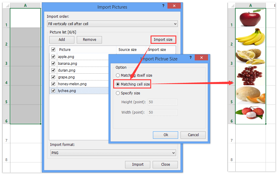
Normally pictures are inserted above cells in Excel. But Kutools for Excel’s Import Pictures utility can help Excel users batch insert each picture/image into a single cell as below screenshot shown:
Go to Download Free Trial 60 daysPurchasePayPal / MyCommerce
Recommended Productivity Software
Office Tab: Use tabbed interface in Office as the use of web browser Chrome, Firefox and Internet Explorer.Kutools for Excel: Adds 120 powerful new features to Excel. Increase your productivity in 5 minutes. Save two hours every day!Classic Menu for Office: Brings back your familiar menus to Office 2007, 2010, 2013 and 2016 (includes Office 365).
 Select all objects in active worksheet

Amazing! Using Tabs in Excel like Firefox, Chrome, Internet Explore 10!
How to be more efficient and save time when using Excel?
You can apply the Go To command to select all objects easily. You can do it with following steps:
Step 1: Press the F5 key to open the Go To dialog box.
Step 2: Click the Special button at the bottom to open the Go To Special dialog box.
Step 3: In the Go To Special dialog box, check the Objects option.
Step 4: Click OK. Then it selects all kinds of objects in active worksheet, including all pictures, all charts, all shapes, and so on.
Select all pictures in active worksheet
It seems no easy way to select all pictures except manually selecting each one. Actually, VB macro can help you to select all pictures in active worksheet quickly.
Step 1: Hold down the ALT + F11 keys, and it opens the Microsoft Visual Basic for Applications window.
Step 2: Click Insert > Module, and paste the following macro in the Module Window.
VBA: Select all pictures in active worksheet
1
2
3
Public Sub SelectAllPics()
ActiveSheet.Pictures.Select
End Sub
Step 3: Press the F5 key to run this macro. Then it selects all pictures in active worksheet immediately.
Select all charts in active worksheet
VB macro can also help you to select all charts in active worksheet too.
Step 1: Hold down the ALT + F11 keys, and it opens the Microsoft Visual Basic for Applications window.
Step 2: Click Insert > Module, and paste the following macro in the Module Window.
VBA: Select all charts in active worksheet
1
2
3
Public Sub SelectAllCharts()
ActiveSheet.ChartObjects.Select
End Sub
Step 3: Press the F5 key to run this macro. This macro will select all kinds of charts in active worksheet in a blink of eyes.
 Quickly delete all objects/ pictures/ charts/ shapes in active/selected/all worksheets
Sometimes, you may need to delete all pictures, charts, or shapes from current worksheet, current workbook or specified worksheets. You can apply Kutools for Excel’s Delete Illustrations & Objects utility to archive it easily.
Kutools for Excel — Combines More Than 120 Advanced Functions and Tools for Microsoft Excel
Go to DownloadFree Trial 60 daysPurchasePayPal / MyCommerce
1. Click Kutools > Delete > Delete Illustrations & Objects.
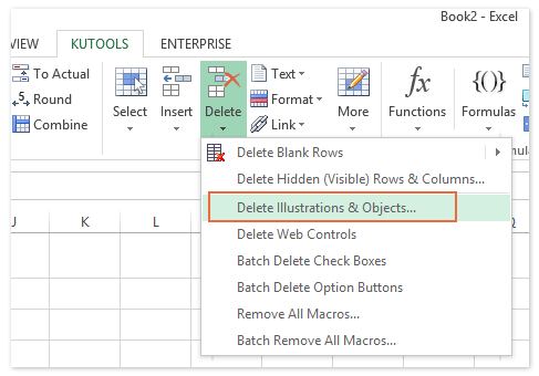
2. In the opening dialog box, you need to:
(1) In the Delete section, please specify the types of objects you want to delete.
In our case, we want to remove charts and pictures, therefore we check the Charts option and Pictures option.
(2) In the Look in section, specify the deleting scope.
In our case, we want to remove charts and pictures from several specified sheets, therefore we check the Selected Sheets option, and then check the specified worksheet in the right box. See left screenshot:
Free Download Kutools for Excel Now
3. Click the Ok button.
Then all charts and pictures are removed from the specified worksheets.
Related Articles
Delete all Pictures easily
Delete all charts Workbooks
Delete all Auto Shapes quickly
Delete all Text Boxes quickly
Is your problem solved?
Yes, I want to be more efficiency and save time when using Excel No, the problem persists and I need further support
Recommended Productivity Tools
The following tools will greatly save your time and effort, which one do you prefer?Office Tab: Using handy tabs in your Office, as the way of Chrome, Firefox and New Internet Explorer.Kutools for Excel: 120 powerful new functions for Excel, Increase your productivity in 5 minutes. Save two hours every day!Classic Menu for Office: Bring back familiar menus to Office 2007, 2010, 2013 and 365, as if it were Office 2000 and 2003.
Kutools for Excel
 Amazing! Increase your productivity in 5 minutes. Don’t need any special skills, save two hours every day!
More than 120 powerful advanced functions which designed for Excel:
- Merge Cell/Rows/Columns without Losing Data.
- Combine and Consolidate Multiple Sheets and Workbooks.
- Compare Ranges, Copy Multiple Ranges, Convert Text to Date, Unit and Currency Conversion.
- Count by Colors, Paging Subtotals, Advanced Sort and Super Filter,
- More Select/Insert/Delete/Text/Format/Link/Comment/Workbooks/Worksheets Tools…

![]()
![]()
![]()
Last updated: January 12, 2017
When you need to make changes that affect multiple cells in Excel, the best way to do so is typically to use your mouse to select all of the cells that you want to modify. But if you need to make a change that affects every cell in your spreadsheet, that is not always the fastest way to select all of the cells. This is especially true when you are working with very large spreadsheets.
But there is a helpful button on an Excel spreadsheet that can help you to select all of the cells in your worksheet very quickly. Out short tutorial below will show you where to find this button.
The steps in this article are going to show you how to select every cell in your spreadsheet. Once all of the cells are selected, you can universally apply changes, such as clearing formatting from the worksheet, or copying all of your data so that it can be pasted into a different spreadsheet. If you need to select all of the worksheets in a workbook, instead of all the cells in a worksheet, then you can continue to the next section.
Step 1: Open your spreadsheet in Excel 2010.
Step 2: Click the button at the top-left corner of the spreadsheet, between the 1 and the A.
You can also select all of the cells in your spreadsheet by clicking on one of the cells in the spreadsheet, then pressing the Ctrl + A keys on your keyboard.
How to Select All in Excel 2010 – How to Select All of the Worksheets in a Workbook
While the above method provides two options for selecting all of the cells in Excel, you might find that you need to select all of the worksheets in a workbook instead. This is helpful when you have a workbook with a lot of different sheets, and you need to make a change that will apply to all of them. Selecting all of the sheets allows you to do perform that change one time, instead of individually for each sheet.
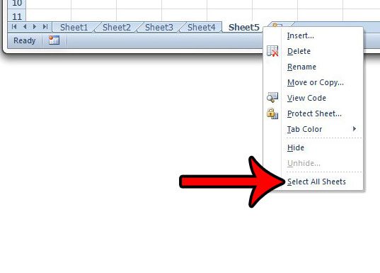
Step 1: Locate the worksheet tabs at the bottom of the window.
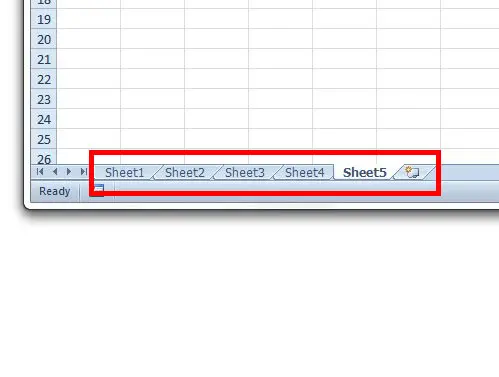
Step 2: Right-click on one of the worksheet tabs, then click the Select All Sheets option.
Is Excel only printing part of your spreadsheet, and you can’t figure out why? Read here to learn about a setting that you should check.

Matthew Burleigh has been writing tech tutorials since 2008. His writing has appeared on dozens of different websites and been read over 50 million times.
After receiving his Bachelor’s and Master’s degrees in Computer Science he spent several years working in IT management for small businesses. However, he now works full time writing content online and creating websites.
His main writing topics include iPhones, Microsoft Office, Google Apps, Android, and Photoshop, but he has also written about many other tech topics as well.
Read his full bio here.
Many users learn early on the “click + hold + drag” method for selecting a range of data using Microsoft Excel. If you have hundreds of rows of data, this method can be very tedious when needing to select all of the data within a worksheet.

3 Different Keyboard Shortcuts to Select “All” Data within a Worksheet
A much easier method to select an entire Excel worksheet is to use the shortcut key Ctrl+A (the “A” stands for “All”). However, your selection may vary:
- When you press Ctrl+A in a worksheet, you are selecting the current range. If there are any blank rows or columns separating the data, the selection area ends: Excel will not select a noncontiguous range.
- If you press Ctrl+A a second time, you’ll select your entire worksheet.
- NOTE: If your data is in a table format, you will need to press Ctrl+A a third time to select the entire worksheet.
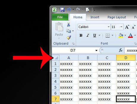
Using Excel’s “Select All” Button to Select All Data
Yet another method for selecting all data in a spreadsheet is to click on the “select all” button at the top left corner of Excel. To the left of column A and above row 1, there is a grey half square looking button:

Using Your Selected Data
With all of your data selected you can:
- Copy and paste the content to a different location within the worksheet or move it to a different worksheet.
- Apply various formatting changes or clear formatting from cells.
- Modify the row height or column widths.
Bonus Tip: Absolute References vs. Relative References
Microassist’s lead instructor, Andy Weaver, talks about absolute and relative references in this virtual class.
Additional Microsoft Excel Resources
This just scratches the surface on what you can learn in Microsoft Excel! We offer multiple courses in Excel, from beginner introductions to Excel to advanced classes, to classes on Pivot Tables and more. Check out our Course Schedule to learn more.
Additional Microsoft Excel Tips
Excel Tip: Speed up Excel Data Entry by Changing Enter Key Behavior
Excel Tip: Highlight All Cells Referenced by a Formula
Excel 2013 Tip: Inserting Comments
NOTE: This post was originally published in December 2008 and has been revamped for currency and accuracy.
Subscribe to Monthly Training Updates
Receive monthly productivity and training insights, software tips, and notices of upcoming classes!