Excel and round function - Word и Excel - помощь в работе с программами

Excel for Microsoft 365 Excel for Microsoft 365 for Mac Excel for the web Excel 2021 Excel 2021 for Mac Excel 2019 Excel 2019 for Mac Excel 2016 Excel 2016 for Mac Excel 2013 Excel 2010 Excel 2007 Excel for Mac 2011 Excel Starter 2010 More…Less

Description

The ROUND function rounds a number to a specified number of digits. For example, if cell A1 contains 23.7825, and you want to round that value to two decimal places, you can use the following formula:

=ROUND(A1, 2)

The result of this function is 23.78.

Syntax

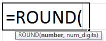
ROUND(number, num_digits)

The ROUND function syntax has the following arguments:

number Required. The number that you want to round.
num_digits Required. The number of digits to which you want to round the number argument.

Remarks

If num_digits is greater than 0 (zero), then number is rounded to the specified number of decimal places.
If num_digits is 0, the number is rounded to the nearest integer.
If num_digits is less than 0, the number is rounded to the left of the decimal point.
To always round up (away from zero), use the ROUNDUP function.
To always round down (toward zero), use the ROUNDDOWN function.
To round a number to a specific multiple (for example, to round to the nearest 0.5), use the MROUND function.

Example

Copy the example data in the following table, and paste it in cell A1 of a new Excel worksheet. For formulas to show results, select them, press F2, and then press Enter. If you need to, you can adjust the column widths to see all the data.

Formula	Description	Result
=ROUND(2.15, 1)	Rounds 2.15 to one decimal place	2.2
=ROUND(2.149, 1)	Rounds 2.149 to one decimal place	2.1
=ROUND(-1.475, 2)	Rounds -1.475 to two decimal places	-1.48
=ROUND(21.5, -1)	Rounds 21.5 to one decimal place to the left of the decimal point	20
=ROUND(626.3,-3)	Rounds 626.3 to the nearest multiple of 1000	1000
=ROUND(1.98,-1)	Rounds 1.98 to the nearest multiple of 10	0
=ROUND(-50.55,-2)	Rounds -50.55 to the nearest multiple of 100	-100

Need more help?

Want more options?

Explore subscription benefits, browse training courses, learn how to secure your device, and more.

Communities help you ask and answer questions, give feedback, and hear from experts with rich knowledge.

Источник

Purpose

Round a number to a given number of digits

Usage notes

The ROUND function rounds a number to a given number of places. ROUND rounds up when the last significant digit is 5 or greater, and rounds down when the last significant digit is less than 5.

ROUND takes two arguments, number and num_digits. Number is the number to be rounded, and num_digits is the place at which number should be rounded. When num_digits is greater than zero, the ROUND function rounds on the right side of the decimal point. When num_digits is less or equal to zero, the ROUND function rounds on the left side of the decimal point. Use zero (0) for num_digits to round to the nearest integer. This behavior is summarized in the table below:

Digits	Behavior
>0	Round to nearest .1, .01, .001, etc.
<0	Round to nearest 10, 100, 1000, etc.
=0	Round to nearest 1

Round to right

To round values to the right of the decimal point, use a positive number for digits:

=ROUND(A1,1) // Round to 1 decimal place
=ROUND(A1,2) // Round to 2 decimal places
=ROUND(A1,3) // Round to 3 decimal places
=ROUND(A1,4) // Round to 4 decimal places

Round to left

To round down values to the left of the decimal point, use zero or a negative number for digits:

=ROUND(A1,0) // Round to nearest whole number
=ROUND(A1,-1) // Round to nearest 10
=ROUND(A1,-2) // Round to nearest 100
=ROUND(A1,-3) // Round to nearest 1000
=ROUND(A1,-4) // Round to nearest 10000

Nesting inside ROUND

Other operations and functions can be nested inside the ROUND function. For example, to round down the result of A1 divided by B1, you can ROUND in a formula like this:

=ROUND(A1/B1,0) // round result to nearest integer

Any formula that returns a numeric result can be nested inside the ROUND function.

Other rounding functions

Excel provides a number of rounding functions, each with a different behavior:

To round with standard rules, use the ROUND function.
To round to the nearest multiple, use the MROUND function.
To round down to the nearest specified place, use the ROUNDDOWN function.
To round down to the nearest specified multiple, use the FLOOR function.
To round up to the nearest specified place, use the ROUNDUP function.
To round up to the nearest specified multiple, use the CEILING function.
To round down and return an integer only, use the INT function.
To truncate decimal places, use the TRUNC function.

Notes

The ROUND function rounds to a specified level of precision, determined by num_digits.
If number is already rounded to the given number of places, no rounding occurs.
If number is not numeric, ROUND returns a #VALUE! error.

Источник

The ROUND Excel function is a built-in function in Excel that calculates the round number of a given number with the number of digits to be provided as an argument. This formula takes two arguments: the number itself and the number of digits to which we want the number to be rounded up.

For example, suppose cell D1 contains 22.5863. Then, if we want to round that value to two decimal places, we can use the following formula: =ROUND(D1,2). As a result, this function may provide 22.59.

ROUND in Excel
- ROUND Formula in Excel
- Usage Notes
- Explanation
- How to Open the ROUND Function in Excel?
- How to Use ROUND Function in Excel with Examples
  - Example #1
  - Example #2
  - Example #3
  - Example #4
  - Example #5
- Other Rounding Functions in Excel
- Things to Remember
- ROUND Excel Function Video
- Recommended Articles

ROUND Formula in Excel

The ROUND Formula in Excel accepts the following parameters and arguments:

Number – The number which has to be rounded.

Num_Digits – The total number of digits to round the number to.

Return Value: The ROUND function returns a numeric value.

Usage Notes

The ROUND formula in Excel works by rounding the numbers 1-4 down and 5-9 up.
You can use the ROUND function in Excel for rounding numbers to a specified level of precision. We can use the ROUND function in Excel for rounding to the right or left of the decimal point.
If num_digits is greater than 0, the number will be rounded to the specified decimal places to the right of the decimal point. For example, =ROUND (16.55, 1) will round 16.55 to 16.6.
If num_digits is less than 0, the number will be rounded to the left of the decimal point (to the nearest 10, 100, 1000, and so on). For example, =ROUND (16.55, -1) will round 16.55 to the nearest 10 and return 20 as the return value or result.
If num_digits = 0, the number will be rounded to the nearest integer (no decimal places). For example, =ROUND (16.55, 0) will round 16.55 to 17.

Explanation

The ROUND in Excel follows the general math rules for rounding the numbers. In this ROUND function, the number to the right of the rounding digit will determine whether the number should be rounded upwards or downwards. The rounding digit is considered the least significant after the number is rounded. It also gets changed, depending on whether the digit following it is less or greater than 5.

If the digit to the right of the rounding digit is 0,1,2,3, or 4, it will not change the rounding digit, and the number will be rounded down.
If the rounding digit is followed by 5,6,7,8 or 9, the rounding digit will be increased by one, and the number will be rounded up.

Consider the following table to understand the above theory more deeply. In this ROUND in Excel example, we are taking the number 106.864. The position is cell number A2 in the spreadsheet.

Formula	Result	Description
=ROUND (A2,2)	106.86	The number in A2 is rounded to 2 decimal places.
=ROUND (A2,1)	106.9	The number is A2 is rounded to 1 decimal place.
=ROUND (A2,0)	107	The number in A2 is rounded to the nearest integer.
=ROUND (A2,-1)	110	The number in A2 is rounded to the nearest multiple of 10.
=ROUND (A2-2)	100	The number in A2 is rounded to the nearest multiple of 100.

How to Open the ROUND Function in Excel?

You can download this ROUND Function Excel Template here – ROUND Function Excel Template

You can insert the desired ROUND formula in the required cell to attain a return value on the argument.
You can manually open the ROUND formula in the Excel dialog box in the spreadsheet and insert the logical values to attain a return value.
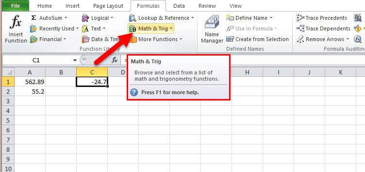
The spreadsheet below shows the “Formulas” section in the “Menu” bar. Under the “Formulas” section, Click on the “Math & Trig.”

After clicking the “Math & Trig option,” select “ROUND.” The ROUND formula in the Excel dialog box will open, as shown below.

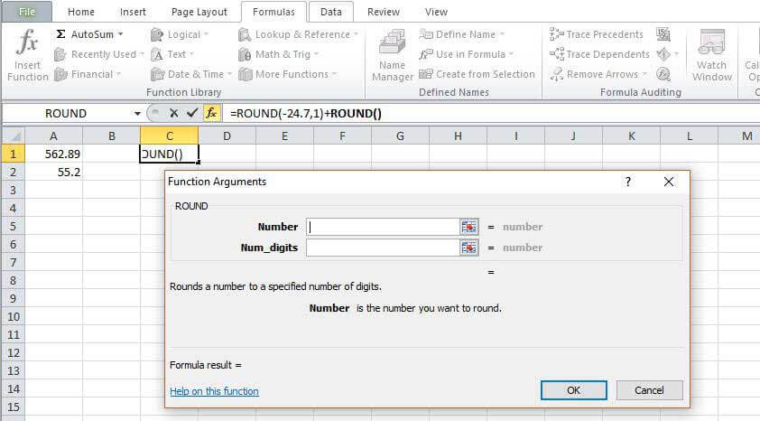
Now, you can easily put the arguments and attain a return value. Just put the required values on Number and Num_digits. You will get the return value.

How to Use ROUND Function in Excel with Examples

Let us look below at some examples of the ROUND formula in Excel. These examples will help you in exploring the use of the ROUND function.

Based on the above Excel spreadsheet, let’s consider three examples and see the ROUND function return based on the syntax of the function.

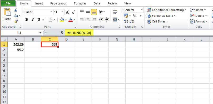
Example #1

When the ROUND formula for Excel written is =ROUND (A1, 0)

Result: 563

You can see the excel spreadsheet below –

Example #2

When the ROUND formula for Excel written is =ROUND (A1, 1)

Result: 562.9

Consider the Excel spreadsheet below-

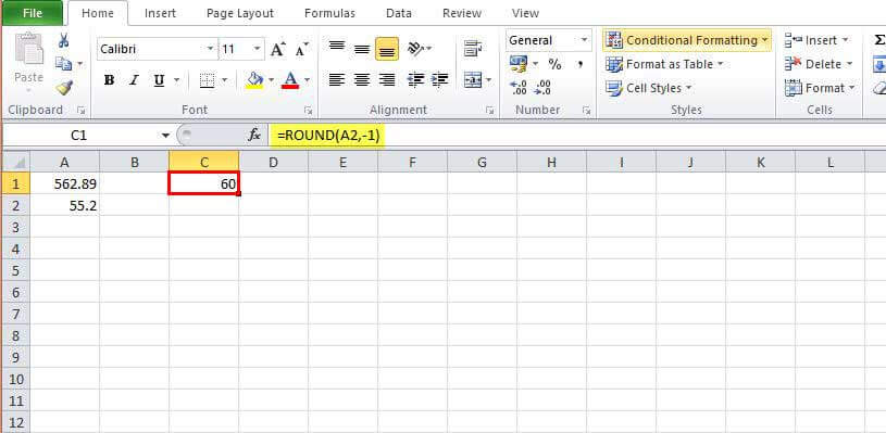
Example #3

When the ROUND formula for Excel written is =ROUND (A2, -1)

Result: 60

Consider the Excel spreadsheet below –

Example #4

When the ROUND formula for Excel is written =ROUND (52.2, -1)

Result: 50

You can consider the excel spreadsheet below –

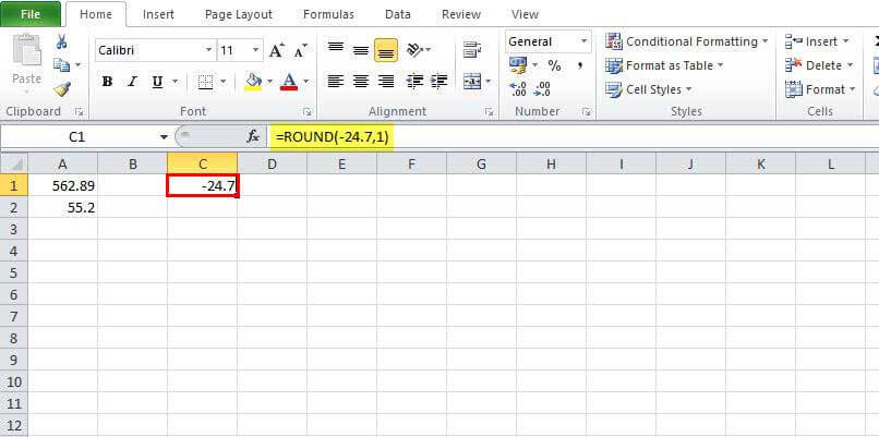
Example #5

When the ROUND formula for Excel is written =ROUND (-24.57, 1)

Result: -24.7

You can see the excel spreadsheet below –

Other Rounding Functions in Excel

You can also force Excel to always round a number up (away from zero) with the help of the ROUNDUP functionThe ROUNDUP excel function calculates the rounded value of the number to the upward side or the higher side. In other words, it rounds the number away from zero. Being an inbuilt function of Excel, it accepts two arguments–the “number” and the “num_of _digits.” For example, “=ROUNDUP(0.40,1)” returns 0.4.
read more. If you want Excel to always round a number down (towards zero), use the ROUNDDOWN function in Excel. For specifying the multiple (example 0.5) that Excel uses to round, use the MROUND function in excelMROUND is the MATH & TRIGNOMETRY function in Excel, and it is used to round a number to the nearest multiple numbers. For example, =MROUND(50,7), will round the number 50 to 49.read more.

Things to Remember

The ROUND function returns a number rounded to a specific number of digits.
The ROUND function is a Math & Trig function.
The ROUND function works by rounding the numbers 1-4 down and 5-9 up.
We can round a number up (away from zero) with the help of the ROUNDUP function.
We can round a number down (towards zero) using the ROUNDDOWN functionROUNDDOWN function is a built-in function in Microsoft Excel. It is used to round off the given number.read more.

ROUND Excel Function Video

Что возвращает функция

Число, округленное, до заданного количества десятичных разрядов.

Больше лайфхаков в нашем Telegram Подписаться

Синтаксис

=ROUND(number, num_digits) — английская версия

=ОКРУГЛ(число;число_разрядов) — русская версия

Аргументы функции

number (число) — число, которое вы хотите округлить;
num_digits (число_разрядов) — значение десятичного разряда, до которого вы хотите округлить первый аргумент функции.

Дополнительная информация

если аргумент num_digits (число_разрядов) больше “0”, то число округляется до указанного количества десятичных знаков. Например, =ROUND(500.51,1) или =ОКРУГЛ(500.51;1) вернет “500.5”;
если аргумент num_digits (число_разрядов) равен “0”, то число округляется до ближайшего целого числа. Например, =ROUND(500.51,0) или =ОКРУГЛ(500.51;0) вернет “501”;
если аргумент num_digits (число_разрядов) меньше “0”, то число округляется влево от десятичного значения. Например, =ROUND(500.51,-1) или =ОКРУГЛ(500.51;-1) вернет “501”.

Примеры использования функции ОКРУГЛ в Excel

Источник

Date yes Add (Subtract) Days to a Date Concatenate Dates Convert Date to Number Convert Date to Text Month Name to Number Create Date Range from Dates Day Number of Year Month Name from Date First Day of Month Add (Subtract) Weeks to a Date If Functions with Dates Max Date Number of Days Between Dates Number of Days in a Month Number of Weeks Between Dates Number of Years Between Dates Split Date & Time into Separate Cells Countdown Remaining Days Insert Dates Random Date Generator Using Dynamic Ranges — Year to Date Values Add (Subtract) Years to a Date Date Formula Examples Extract Day from Date Get Day Name from Date Count Days Left in Month / Year Count Workdays Left in Month / Year Get Last Day of Month Last Business Day of Month / Year Number of Work / Business Days in Month Weekday Abbreviations Auto Populate Dates Number of Months Between Dates Quarter from a Date Years of Service Change Date Format Compare Dates Time yes Add (Subtract) Hours to Time Add (Subtract) Minutes to Time Add (Subtract) Seconds to Time Add Up time (Total Time) Time Differences Change Time Format Convert Minutes to Hours Convert Time to Decimal Convert Time to Hours Convert Time to Minutes Convert Time to Seconds Military Time Round Time to Nearest 15 Minutes Overtime Calculator Number of Hours Between Times Convert Seconds to Minutes, Hours, or Time Count Hours Worked Time Differences Time Format — Show Minutes Seconds Text yes Add Commas to Cells Get First Word from Text Capitalize First Letter Clean & Format Phone #s Remove Extra Trailing / Leading Spaces Add Spaces to Cell Assign Number Value to Text Combine Cells with Comma Combine First and Last Names Convert Text String to Date Convert Text to Number Extract Text From Cell Get Last Word Remove Unwated Characters Extract Text Before or After Character How to Split Text String by Space, Comma, & More Remove Special Characters Remove First Characters from Left Substitute Multiple Values Switch First & Last Names w/ Commas Remove Specific Text from a Cell Extract Text Between Characters (Ex. Parenthesis) Add Leading Zeros to a Number Remove Line Breaks from Text Remove all Numbers from Text Reverse Text Remove Non-Numeric Characters Remove Last Character(s) From Right Separate First and Last Names Separate Text & Numbers Round yes Round Formulas Round Price to Nearest Dollar or Cent Round to Nearest 10, 100, or 1000 Round to Nearest 5 or .5 Round Percentages Round to Significant Figures Count yes Count Blank and Non-blank Cells Count Cells Between Two Numbers Count Cells not Equal to Count if Cells are in Range Count Times Word Appears in Cell Count Words in Cell Count Specific Characters in Column Count Total Number of Characters in Column Count Cells that Equal one of two Results Count Cells that do not Contain Count Cells that Contain Specific Text Count Unique Values in Range Countif — Multiple Criteria Count Total Number of Cells in Range Count Cells with Any Text Count Total Cells in a Table Lookup yes Two Dimensional VLOOKUP VLOOKUP Simple Example Vlookup — Multiple Matches Case Sensitive Lookup Case Sensitive VLOOKUP Sum if — VLOOKUP Case Sensitive Lookup Case Sensitive VLOOKUP Find Duplicates w/ VLOOKUP or MATCH INDEX MATCH MATCH Lookup — Return Cell Address (Not Value) Lookup Last Value in Column or Row Reverse VLOOKUP (Right to Left) Risk Score Bucket with VLOOKUP Sum with a VLOOKUP Function VLOOKUP & INDIRECT VLOOKUP Concatenate VLOOKUP Contains (Partial Match) 17 Reasons Why Your XLOOKUP is Not Working Double (Nested) XLOOKUP — Dynamic Columns IFERROR (& IFNA) XLOOKUP Lookup Min / Max Value Nested VLOOKUP Top 11 Alternatives to VLOOKUP (Updated 2022!) VLOOKUP – Dynamic Column Reference VLOOKUP – Fix #N/A Error VLOOKUP – Multiple Sheets at Once VLOOKUP & HLOOKUP Combined VLOOKUP & MATCH Combined VLOOKUP Between Worksheets or Spreadsheets VLOOKUP Duplicate Values VLOOKUP Letter Grades VLOOKUP Return Multiple Columns VLOOKUP Returns 0? Return Blank Instead VLOOKUP w/o #N/A Error XLOOKUP Multiple Sheets at Once XLOOKUP Between Worksheets or Spreadsheets XLOOKUP by Date XLOOKUP Duplicate Values XLOOKUP Multiple Criteria XLOOKUP Return Multiple Columns XLOOKUP Returns 0? Return Blank Instead XLOOKUP Text XLOOKUP with IF XLOOKUP With If Statement Misc. yes Sort Multiple Columns Use Cell Value in Formula Percentage Change Between Numbers Percentage Breakdown Rank Values Add Spaces to Cell CAGR Formula Average Time Decimal Part of Number Integer Part of a Number Compare Items in a List Dealing with NA() Errors Get Worksheet Name Wildcard Characters Hyperlink to Current Folder Compound Interest Formula Percentage Increase Create Random Groups Sort with the Small and Large Functions Non-volatile Function Alternatives Decrease a Number by a Percentage Calculate Percent Variance Profit Margin Calculator Convert Column Number to Letter Get Full Address of Named Range Insert File Name Insert Path Latitute / Longitude Functions Replace Negative Values Reverse List Range Convert State Name to Abbreviation Create Dynamic Hyperlinks Custom Sort List with Formula Data Validation — Custom Formulas Dynamic Sheet Reference (INDIRECT) Reference Cell in Another Sheet or Workbook Get Cell Value by Address Get Worksheet Name Increment Cell Reference List Sheet Names List Skipped Numbers in Sequence Return Address of Max Value in Range Search by Keywords Select Every Other (or Every nth) Row Basics yes Cell Reference Basics — A1, R1C1, 3d, etc. Add Up (Sum) Entire Column or Row Into to Dynamic Array Formulas Conversions yes Convert Time Zones Convert Celsius to Fahrenheit Convert Pounds to Kilograms Convert Time to Unix Time Convert Feet to Meters Convert Centimeters to Inches Convert Kilometers to Miles Convert Inches to Feet Convert Date to Julian Format Convert Column Letter to Number Tests yes Test if a Range Contains any Text Test if any Cell in Range is Number Test if a Cell Contains a Specific Value Test if Cell Contains Any Number Test if Cell Contains Specific Number Test if Cell is Number or Text If yes Percentile If Subtotal If Sumproduct If Large If and Small If Median If Concatentate If Max If Rank If TEXTJOIN If Sum yes Sum if — Begins With / Ends With Sum if — Month or Year to Date Sum if — By Year Sum if — Blank / Non-Blank Sum if — Horizontal Sum Count / Sum If — Cell Color INDIRECT Sum Sum If — Across Multiple Sheets Sum If — By Month Sum If — Cells Not Equal To Sum If — Not Blank Sum if — Between Values Sum If — Week Number Sum Text Sum if — By Category or Group Sum if — Cell Contains Specific Text (Wildcards) Sum if — Date Rnage Sum if — Dates Equal Sum if — Day of Week Sum if — Greater Than Sum if — Less Than Average yes Average Non-Zero Values Average If — Not Blank Average — Ignore 0 Average — Ignore Errors Math yes Multiplication Table Cube Roots nth Roots Square Numbers Square Roots Calculations yes Calculate a Ratio Calculate Age KILLLLLLL Calculate Loan Payments GPA Formula Calculate VAT Tax How to Grade Formulas Find yes Find a Number in a Column / Workbook Find Most Frequent Numbers Find Smallest n Values Find nth Occurance of Character in Text Find and Extract Number from String Find Earliest or Latest Date Based on Criteria Find First Cell with Any Value Find Last Row Find Last Row with Data Find Missing Values Find Largest n Values Most Frequent Number Conditional Formatting yes Conditional Format — Dates & Times Conditional Format — Highlight Blank Cells New Functions XLOOKUP Replaces VLOOKUP, HLOOKUP, and INDEX / MATCH Logical yes AND Checks whether all conditions are met. TRUE/FALSE IF If condition is met, do something, if not, do something else. IFERROR If result is an error then do something else. NOT Changes TRUE to FALSE and FALSE to TRUE. OR Checks whether any conditions are met. TRUE/FALSE XOR Checks whether one and only one condition is met. TRUE/FALSE Lookup & Reference yes FALSE The logical value: FALSE. TRUE The logical value: TRUE. ADDRESS Returns a cell address as text. AREAS Returns the number of areas in a reference. CHOOSE Chooses a value from a list based on it’s position number. COLUMN Returns the column number of a cell reference. COLUMNS Returns the number of columns in an array. HLOOKUP Lookup a value in the first row and return a value. HYPERLINK Creates a clickable link. INDEX Returns a value based on it’s column and row numbers. INDIRECT Creates a cell reference from text. LOOKUP Looks up values either horizontally or vertically. MATCH Searches for a value in a list and returns its position. OFFSET Creates a reference offset from a starting point. ROW Returns the row number of a cell reference. ROWS Returns the number of rows in an array. TRANSPOSE Flips the oriention of a range of cells. VLOOKUP Lookup a value in the first column and return a value. Date & Time yes DATE Returns a date from year, month, and day. DATEDIF Number of days, months or years between two dates. DATEVALUE Converts a date stored as text into a valid date DAY Returns the day as a number (1-31). DAYS Returns the number of days between two dates. DAYS360 Returns days between 2 dates in a 360 day year. EDATE Returns a date, n months away from a start date. EOMONTH Returns the last day of the month, n months away date. HOUR Returns the hour as a number (0-23). MINUTE Returns the minute as a number (0-59). MONTH Returns the month as a number (1-12). NETWORKDAYS Number of working days between 2 dates. NETWORKDAYS.INTL Working days between 2 dates, custom weekends. NOW Returns the current date and time. SECOND Returns the second as a number (0-59) TIME Returns the time from a hour, minute, and second. TIMEVALUE Converts a time stored as text into a valid time. TODAY Returns the current date. WEEKDAY Returns the day of the week as a number (1-7). WEEKNUM Returns the week number in a year (1-52). WORKDAY The date n working days from a date. WORKDAY.INTL The date n working days from a date, custom weekends. YEAR Returns the year. YEARFRAC Returns the fraction of a year between 2 dates. Engineering yes CONVERT Convert number from one unit to another. Financial yes FV Calculates the future value. PV Calculates the present value. NPER Calculates the total number of payment periods. PMT Calculates the payment amount. RATE Calculates the interest Rate. NPV Calculates the net present value. IRR The internal rate of return for a set of periodic CFs. XIRR The internal rate of return for a set of non-periodic CFs. PRICE Calculates the price of a bond. YIELD Calculates the bond yield. INTRATE The interest rate of a fully invested security. Information yes CELL Returns information about a cell. ERROR.TYPE Returns a value representing the cell error. ISBLANK Test if cell is blank. TRUE/FALSE ISERR Test if cell value is an error, ignores #N/A. TRUE/FALSE ISERROR Test if cell value is an error. TRUE/FALSE ISEVEN Test if cell value is even. TRUE/FALSE ISFORMULA Test if cell is a formula. TRUE/FALSE ISLOGICAL Test if cell is logical (TRUE or FALSE). TRUE/FALSE ISNA Test if cell value is #N/A. TRUE/FALSE ISNONTEXT Test if cell is not text (blank cells are not text). TRUE/FALSE ISNUMBER Test if cell is a number. TRUE/FALSE ISODD Test if cell value is odd. TRUE/FALSE ISREF Test if cell value is a reference. TRUE/FALSE ISTEXT Test if cell is text. TRUE/FALSE N Converts a value to a number. NA Returns the error: #N/A. TYPE Returns the type of value in a cell. Math yes ABS Calculates the absolute value of a number. AGGREGATE Define and perform calculations for a database or a list. CEILING Rounds a number up, to the nearest specified multiple. COS Returns the cosine of an angle. DEGREES Converts radians to degrees. DSUM Sums database records that meet certain criteria. EVEN Rounds to the nearest even integer. EXP Calculates the exponential value for a given number. FACT Returns the factorial. FLOOR Rounds a number down, to the nearest specified multiple. GCD Returns the greatest common divisor. INT Rounds a number down to the nearest integer. LCM Returns the least common multiple. LN Returns the natural logarithm of a number. LOG Returns the logarithm of a number to a specified base. LOG10 Returns the base-10 logarithm of a number. MOD Returns the remainder after dividing. MROUND Rounds a number to a specified multiple. ODD Rounds to the nearest odd integer. PI The value of PI. POWER Calculates a number raised to a power. PRODUCT Multiplies an array of numbers. QUOTIENT Returns the integer result of division. RADIANS Converts an angle into radians. RAND Calculates a random number between 0 and 1. RANDBETWEEN Calculates a random number between two numbers. ROUND Rounds a number to a specified number of digits. ROUNDDOWN Rounds a number down (towards zero). ROUNDUP Rounds a number up (away from zero). SIGN Returns the sign of a number. SIN Returns the sine of an angle. SQRT Calculates the square root of a number. SUBTOTAL Returns a summary statistic for a series of data. SUM Adds numbers together. SUMIF Sums numbers that meet a criteria. SUMIFS Sums numbers that meet multiple criteria. SUMPRODUCT Multiplies arrays of numbers and sums the resultant array. TAN Returns the tangent of an angle. TRUNC Truncates a number to a specific number of digits. Stats yes AVERAGE Averages numbers. AVERAGEA Averages numbers. Includes text & FALSE =0, TRUE =1. AVERAGEIF Averages numbers that meet a criteria. AVERAGEIFS Averages numbers that meet multiple criteria. CORREL Calculates the correlation of two series. COUNT Counts cells that contain a number. COUNTA Count cells that are non-blank. COUNTBLANK Counts cells that are blank. COUNTIF Counts cells that meet a criteria. COUNTIFS Counts cells that meet multiple criteria. FORECAST Predict future y-values from linear trend line. FREQUENCY Counts values that fall within specified ranges. GROWTH Calculates Y values based on exponential growth. INTERCEPT Calculates the Y intercept for a best-fit line. LARGE Returns the kth largest value. LINEST Returns statistics about a trendline. MAX Returns the largest number. MEDIAN Returns the median number. MIN Returns the smallest number. MODE Returns the most common number. PERCENTILE Returns the kth percentile. PERCENTILE.INC Returns the kth percentile. Where k is inclusive. PERCENTILE.EXC Returns the kth percentile. Where k is exclusive. QUARTILE Returns the specified quartile value. QUARTILE.INC Returns the specified quartile value. Inclusive. QUARTILE.EXC Returns the specified quartile value. Exclusive. RANK Rank of a number within a series. RANK.AVG Rank of a number within a series. Averages. RANK.EQ Rank of a number within a series. Top Rank. SLOPE Calculates the slope from linear regression. SMALL Returns the kth smallest value. STDEV Calculates the standard deviation. STDEV.P Calculates the SD of an entire population. STDEV.S Calculates the SD of a sample. STDEVP Calculates the SD of an entire population TREND Calculates Y values based on a trendline. Text yes CHAR Returns a character specified by a code. CLEAN Removes all non-printable characters. CODE Returns the numeric code for a character. CONCATENATE Combines text together. DOLLAR Converts a number to text in currency format. EXACT Test if cells are exactly equal. Case-sensitive. TRUE/FALSE FIND Locates position of text within a cell.Case-sensitive. LEFT Truncates text a number of characters from the left. LEN Counts number of characters in text. LOWER Converts text to lower case. MID Extracts text from the middle of a cell. PROPER Converts text to proper case. REPLACE Replaces text based on it’s location. REPT Repeats text a number of times. RIGHT Truncates text a number of characters from the right. SEARCH Locates position of text within a cell.Not Case-sensitive. SUBSTITUTE Finds and replaces text. Case-sensitive. TEXT Converts a value into text with a specific number format. TRIM Removes all extra spaces from text. UPPER Converts text to upper case. VALUE Converts a number stored as text into a number.

Источник

Microsoft Excel provides multiple formulas to round numbers. We have formulas like – ROUND, ROUNDUP, ROUNDDOWN, MROUND, INT, TRUNC, CEILING, FLOOR, FIXED, EVEN, ODD, and they all can be used to round numbers in excel.

Rounding is the process of removing the least significant digits from a number so that we are left with a simpler value that is very close to the original number.

In short, rounding gives you an approximate value that is quite accurate.

ROUND Function In Excel
- Syntax
Round to Right
- Example 1: Use the Excel Round Function to round a number to 3 decimal places.
- Example 2: Use the Round Function in Excel to round a number to 2 decimal places.
Round to Left
- Example 3: Use the Excel Round Function to round a number to the nearest 10.
- Example 4: Use the Round Function in Excel to round a number to the nearest 100.
- Example 5: Use the Excel Round Function to round a number to the nearest whole number.
- Example 6: Use the Round Function in Excel to round a negative number to the nearest integer.
Nesting Inside Excel Round Function
- Example 7: Use Excel Round Function to round sum of two numbers
- Example 8: Use Round Function in Excel to round the division quotient of 2 numbers
ROUNDDOWN Function In Excel
- Syntax:
- Example 9: Use ROUNDDOWN Function in Excel to round a number down to 3 decimal places.
- Example 10: Use Excel ROUNDDOWN Function to round a number to the nearest integer.
- Example 11: Use ROUNDDOWN Function in Excel to round a number down to the nearest 10.
- Example 12: Use Excel ROUNDDOWN Function to round a number down to the nearest 100.
- Example 13: Use ROUNDDOWN Function in Excel to round a negative number down to 2 decimal places.
- Example 14: Use Excel ROUNDDOWN Function to round a negative number down to the nearest integer.
ROUNDUP Function In Excel
- Syntax:
- Example 15: Use ROUNDUP Function in Excel to round a number up to 3 decimal places.
- Example 16: Use Excel ROUNDUP Function to round a number up to 1 decimal place.
- Example 17: Use ROUNDUP Function in Excel to round a number up to the nearest integer.
- Example 18: Use Excel ROUNDUP Function to round a number up to the nearest 10.
- Example 19: Use ROUNDUP Function in Excel to round a number up to the nearest 100.
- Example 20: Use Excel ROUNDUP Function to round a negative number to 1 decimal place.
- Example 21: Use ROUNDUP Function in Excel to round a negative number up to the nearest integer.
MROUND Function In Excel
- Syntax:
- Example 22: Use MROUND Function in Excel to round a number to the nearest multiple of 2
- Example 23: Use Excel MROUND Function to round a number to the nearest multiple of 0.5
FLOOR Function In Excel
- Syntax:
- Some rules for using the FLOOR function:
- Example 24: Round a number down to the nearest multiple of 2.
- Example 25: Round a number down to the nearest multiple of 0.5
- Example 26: Round a negative number down to the nearest multiple of 3
- Example 27: Round a number down to the nearest multiple of -2.
CEILING Function In Excel
- Syntax:
- Some rules for using the CEILING function:
- Example 28: Round a number up to the nearest multiple of 5
- Example 29: Round a number up to the nearest multiple of 0.5
- Example 30: Round a negative number up to the nearest multiple of 6.
- Example 31: Round a number up to the nearest multiple of -5
- Example 32: Round a negative number to the nearest multiple of -2.
INT Function In Excel
- Syntax:
- Example 33: Round down a positive number
- Example 34: Round down a negative number
TRUNC Function In Excel
- Syntax:
- Some rules for using the TRUNC Function:
- TRUNC V/S INT
- Example 35: Truncate a number 2 decimal places to the right
- Example 36: Truncate a negative number 1 decimal to the left.
- Example 37: Truncate the number to the nearest integer.
Even Function In Excel
- Syntax:
- Example 38: Round up an odd positive number
- Example 39: Round up an odd negative number
- Example 40: Round up an even positive number
Odd Function In Excel
- Syntax:
- Example 41: Round up an even positive number
- Example 42: Round up an even negative number
- Example 43: Round up an odd positive number

ROUND Function In Excel

The ROUND function is the most popular rounding function in excel. Round Function can round a number to the right or left of the decimal point.

Syntax

=ROUND(number, num_digits)

Here, ‘number’ represents the value that needs to be rounded. This is a required parameter. This can be any real number; it can also be a reference to a cell containing a number.

The ‘num_digits’ argument is also a required parameter. This signifies the number of digits to which you want to round the number argument. This can take a value that is positive, negative, or zero.

If ‘num_digits’ is positive or greater than zero, the number is rounded to a specified number of decimal places.
If ‘num_digits’ is negative or less than zero, the number is rounded to the left of the decimal point.
If ‘num_digits’ is zero, the number is rounded to the nearest whole number or integer.

Note: If the number is already rounded to the given number of places, then no rounding occurs, and its value stays the same.

Now, let’s see some examples of the ROUND function in excel and try to understand how to use ROUND function in excel.

Round to Right

In order to round the specified ‘number’ to the right of the decimal point, the ‘num_digits’ parameter should have a positive value.

Example 1: Use the Excel Round Function to round a number to 3 decimal places.

Consider rounding the number 5792.584345 (present in the cell A3) to 3 decimal places.

The formula would be as follows:

=ROUND(A3, 3)

The result is 5792.584 since the number to the right of 4 is 3, so the rounding digit does not change.

Example 2: Use the Round Function in Excel to round a number to 2 decimal places.

Round the number 43.47894 (present in cell A4) to 2 decimal places.

The formula would be as follows:

=ROUND(A4, 2)

The result is 43.479 since the number to the right of 8 is 9, so the rounding digit is increased by one.

Round to Left

In order to round the specified ‘number’ to the left of the decimal point, the ‘num_digits’ parameter should have a negative value.

Example 3: Use the Excel Round Function to round a number to the nearest 10.

We need to round the number 6593.578 (present in the cell A9) to the nearest 10.

The formula would be as follows:

=ROUND(A9,-1)

‘num_digits’ parameter, in this case, is -1, which means rounding needs to be done to the nearest 10, and hence the result is 6590.

Example 4: Use the Round Function in Excel to round a number to the nearest 100.

Round the number 5689.56 (present in cell A10) to the nearest 100.

The formula would be as follows:

=ROUND(A10,-2)

‘num_digits’ parameter, in this case, is -2, which means rounding needs to be done to the nearest 100, and hence the result is 5700.

Similarly, to round any number to the nearest 1000, the value of the ‘num_digits’ parameter should be -3 and so on.

Example 5: Use the Excel Round Function to round a number to the nearest whole number.

Round the number 68.394 (present in cell A11) to the nearest whole number.

The formula would be as follows:

=ROUND(A11,0)

‘num_digits’ parameter, in this case, is 0, which means rounding needs to be done to the nearest 1, and hence the result is 68.

Example 6: Use the Round Function in Excel to round a negative number to the nearest integer.

Round the number -58.69 (present in the cell A12) to the nearest integer.

The formula for this problem would be as follows:

=ROUND(A12,0)

Like Example 5, in this case, the ‘num_digits’ parameter is 0, which means that the rounding needs to be done to the nearest 1, and hence the result is -58.

Nesting Inside Excel Round Function

Other functions that return a numeric result can be nested within the ROUND function. This can help in using the ROUND function as part of a more complicated formula.

Example 7: Use Excel Round Function to round sum of two numbers

Round the result of the sum of two numbers 5869.548 and 5781.579 (present in cells A17and B17 respectively) to 1 decimal place.

The formula would be as follows:

=ROUND(A17+B17,1)

The result of A17 +B17 = 11,651.127 and rounding it to 1 decimal place results in 11564.1.

Example 8: Use Round Function in Excel to round the division quotient of 2 numbers

Round the division quotient of 2 numbers 669.547 and 61.578 (present in cells A18 and B18, respectively) to the nearest integer.

The formula would be as follows:

=ROUND(A18/B18,0)

The quotient A18/B18 = 10.8731527493585, and rounding it to the nearest one results in 11.

ROUNDDOWN Function In Excel

The ROUNDDOWN Function in Excel rounds down a given number to the specified number of decimal places.

The main difference between the ROUNDDOWN Function and ROUND Function is – In the ROUND function, the result depends on the rounding digit’s value. If it is less than five, then the number is rounded down; else, it is rounded up.

However, in the case of the ROUNDDOWN Function, the specified number is always rounded downwards.

Syntax:

=ROUNDDOWN(number, num_digits)

Here, ‘number’ represents the number that needs to be rounded. This is a required parameter. This can be any real number; it can also be a reference to a cell containing a number.

The ‘num_digits’ argument is also a required parameter. This signifies the number of digits to which you want to round the number argument. This can take on a value that is positive, negative, or zero.

Example 9: Use ROUNDDOWN Function in Excel to round a number down to 3 decimal places.

We want to round the number 589.125678 (present in cell A23) down to 3 decimal places.

The formula would be as follows:

=ROUNDDOWN(A23,3)

And the result is 569.125. Even if the rounding digit is followed by a number greater than 5, the rounding number is retained.

Example 10: Use Excel ROUNDDOWN Function to round a number to the nearest integer.

Round a number 45710.265 (present in cell A24) down to the nearest integer.

The formula for this would be as follows:

=ROUNDDOWN(A24,0)

Resulting in 45710.

Example 11: Use ROUNDDOWN Function in Excel to round a number down to the nearest 10.

Consider rounding the number 548.256 (present in cell A25) down to the nearest 10.

The formula would be as follows:

=ROUNDDOWN(A25,-1)

And the result would be 540.

Note that even though the rounding number 4 is followed by a number greater than 5, however, ROUNDDOWN Function does not consider this and simply rounds down the number to the nearest 10.

Example 12: Use Excel ROUNDDOWN Function to round a number down to the nearest 100.

In this example, we need to round the number 2579.457 (present in the cell A26) down to the nearest 100.

The formula for this would be as follows:

=ROUNDDOWN(A26,-2)

Resulting in 2500. Even though the rounding number 5 is followed by 7, the number gets rounded down to 2500.

Example 13: Use ROUNDDOWN Function in Excel to round a negative number down to 2 decimal places.

We have to round -576.5783 (present in cell A27) down to 2 decimal places.

The formula would be as follows:

=ROUNDDOWN(A27,2)

Resulting in a value -576.57.

Example 14: Use Excel ROUNDDOWN Function to round a negative number down to the nearest integer.

So here we have to round -2576.54 (present in cell A28) down to the nearest integer.

The formula would be as follows:

=ROUNDDOWN(A28,0)

Resulting in -2576.

In this case, ROUNDDOWN Function first finds the absolute value of the given number, which is 2576.54, then rounds it down to the nearest integer, which results in 2576. Finally, it affixes the negative sign, which gives -2576.

ROUNDUP Function In Excel

The ROUNDUP function in Excel rounds up a given number to the specified number of decimal places. It is just opposite to the ROUNDDOWN Function.

The main difference between the ROUNDUP function and ROUND the Function is – In the ROUND function, the result depends on the rounding digit’s value. If it is greater than or equal to 5, then the number is rounded up; else, it is rounded down.

However, in the case of the ROUNDUP function, the specified number is always rounded upwards.

Syntax:

=ROUNDUP (number, num_digits)

Here, ‘number’ represents the number that needs to be rounded. This is a required parameter. This can be any real number; it can also be a reference to a cell containing a number.

Example 15: Use ROUNDUP Function in Excel to round a number up to 3 decimal places.

We need to round 478.59786 (present in cell A33) up to 3 decimal places in this example.

The formula would be as follows:

=ROUNDUP(A33,3)

Resulting in 478.598.

Here the rounding number 7 is increased by one, so it is replaced by the number 8 to give the result.

Example 16: Use Excel ROUNDUP Function to round a number up to 1 decimal place.

Consider rounding a number 58.5245 (present in cell A34) up to 1 decimal place.

The formula for this would be as follows:

=ROUNDUP(A34,1)

And the result is 58.6.

Note that even though the rounding digit five is followed by 2, the value is not retained but increases by 1, resulting in 6 after the decimal point.

Example 17: Use ROUNDUP Function in Excel to round a number up to the nearest integer.

We need to round 576.35 (present in cell A35) up to the nearest integer.

The formula would be as follows:

=ROUNDUP(A35,0)

Resulting in 577.

Example 18: Use Excel ROUNDUP Function to round a number up to the nearest 10.

We need to round a number 5862.12 (present in cell A36) up to the nearest 10.

The formula would be as follows:

=ROUNDUP(A36,-1)

And the result would be 5870.

In this example, rounding number 6 is rounded up to the nearest 10, thereby giving the result as 5870.

Example 19: Use ROUNDUP Function in Excel to round a number up to the nearest 100.

We need to round a number 5868.5757 (present in cell A37) up to the nearest 100.

The formula would be as follows:

=ROUNDUP(A37,-2)

And the result is 5900. The rounding digit 8 is rounded up to the nearest 100, thereby giving the result as 5900.

Example 20: Use Excel ROUNDUP Function to round a negative number to 1 decimal place.

We need to round a number -6485.56 (present in cell A38) up to 1 decimal place.

The formula would be as follows:

=ROUNDUP(A38,1)

And the result is -6485.6, the rounding digit 5 is increased by 1.

Example 21: Use ROUNDUP Function in Excel to round a negative number up to the nearest integer.

We need to round a number -472.25 present in cell A39 up to the nearest integer.

The formula would be as follows:

=ROUNDUP(A39,0)

And the result is -473.

In this case, the ROUNDUP function first takes the absolute value of the number, which is 472.25, and rounds it up to the nearest integer, 473, then affixes the negative sign for the final result -473.

MROUND Function In Excel

The MROUND Function is used for rounding a number to the nearest multiple. So, this Function will round a number up or down depending on the nearest multiple.

Syntax:

=MROUND(number, multiple)

‘number’ signifies the number or the cell value that needs to be rounded.

‘multiple’ is the multiple you want to round your number to.

The last remaining digit can be rounded up (away from zero) or down (towards zero) depending on the remainder obtained by dividing the number by the multiple.

If the value of the remainder is equal to or greater than half of the multiple, then the MROUND Function rounds up the last digit.
If the value of the remainder is less than half the multiple, then the last digit is rounded down.

Let’s understand this with the help of some examples:

Example 22: Use MROUND Function in Excel to round a number to the nearest multiple of 2

In this example, we need to round 583 (present in the cell A44) to the nearest multiple of 2.

The formula for this would be as follows:

=MROUND(A44,2)

Now let’s try to find out the result – The nearest multiple of 2 can either be 584 or 582. Which one will it be?

If we divide the number (583) by the multiple (2), we get 291 as quotient and 1 as remainder. Since the remainder 1 is equal to half of the multiple (2) so, the number is rounded upwards to 584.

Example 23: Use Excel MROUND Function to round a number to the nearest multiple of 0.5

Let’s say we need to round a number 583.58 (present in cell A45) to the nearest multiple of 0.5.

The formula would be as follows:

=MROUND(A45,0.5)

Now let’s get to the result – The nearest multiple of 0.5 can either be 583.5 or 584.

If you divide 583.58 by 0.5, the quotient is 1167, and the remainder is 0.080, and since the remainder is less than half the multiple, so the final result is 583.5.

FLOOR Function In Excel

The Excel FLOOR function is used for rounding a number down to the nearest specific multiple. It is similar to the Excel MROUND function except that it always rounds the number downwards.

Syntax:

=FLOOR(number, significance)

‘number’ signifies the number or the cell value that needs to be rounded.

‘significance’ is the multiple you want to round your number to.

Some rules for using the FLOOR function:

If both the ‘number’ and ‘significance’ are greater than 0, then the number is rounded down toward zero.
If the ‘number’ is positive, but ‘significance’ is negative, then the result will be an error #NUM.
If the ‘number’ is negative and ‘significance’ is positive, then the value is rounded away from zero.

Note: If you are using Excel 2003 and 2007, both the ‘number’ and significance’ must have the same sign, or else it will come out as an error. In later Excel versions, there is an improvement in the FLOOR function, and it can handle a negative number with a positive significance.

Example 24: Round a number down to the nearest multiple of 2.

Consider rounding a number 839 (present in cell A50) down to the nearest multiple of 2.

The formula would be as follows:

=FLOOR(A50,2)

And the result would be 838 (not 840) since the number is rounded downwards.

Example 25: Round a number down to the nearest multiple of 0.5

We need to round 9763.9 (present in cell A51) down to the nearest multiple of 0.5.

The formula would be as follows:

=FLOOR(A51,5)

And the result is 9763.5

Example 26: Round a negative number down to the nearest multiple of 3

Round the number -57894 (present in cell A52) to the nearest multiple of 3.

The formula would be as follows:

=FLOOR(A52,3)

And the result is -57894 since the number is a multiple of 3; hence it is not rounded down.

Example 27: Round a number down to the nearest multiple of -2.

Round the number 167 (present in the cell A53) to the nearest multiple of -2.

The formula would be as follows:

=FLOOR(A53,-2)

Since the significance is negative and the number is positive, the result is #NUM error.

CEILING Function In Excel

The Excel CEILING function is used for rounding a number upwards to the nearest specific multiple. It is similar to the Excel MROUND function except that it always rounds the number upwards.

Syntax:

=CEILING(number, significance)

‘number’ signifies the number or the cell value that needs to be rounded.

‘significance’ is the multiple you want to round your number to.

Rounding with Excel CEILING function is similar to the FLOOR function except that the number is rounded up or away from zero instead of down.

Some rules for using the CEILING function:

IF both arguments are positive, then the number is rounded up to the nearest multiple.
If the ‘number’ is positive, and the ‘significance’ is negative, the CEILING function will result in an error #NUM.
A negative ‘number’ with a positive ‘significance’ will also be rounded up.
If both the ‘number’ and ‘significance’ are negative, then the number is rounded down.

Example 28: Round a number up to the nearest multiple of 5

We need to round the number 4753 (present in the cell A58) up to the nearest multiple of 5.

The formula would be as follows:

=CEILING(A58,5)

And the result is 4755 (not 4750) since the number is rounded up.

Example 29: Round a number up to the nearest multiple of 0.5

Consider rounding a number 589.29 (present in the cell A59) up to the nearest multiple of 0.5.

The formula would be as follows:

=CEILING(A59,0.5)

And the result is 589.5

Example 30: Round a negative number up to the nearest multiple of 6.

Let’s say we need to round -3647 (present in the cell A60) up to the nearest multiple of 6.

The formula would be as follows:

=CEILING(A60,6)

And the result is -3642

Example 31: Round a number up to the nearest multiple of -5

Let’s consider rounding a number 7348 (present in the cell A61) up to the nearest multiple of -5.

The formula for this would be as follows:

=CEILING(A61,-5)

And the result is the #NUM error since the CEILING function results in an error #NUM error if the ‘number’ is positive, and the ‘significance’ is negative.

Example 32: Round a negative number to the nearest multiple of -2.

Round the number -6847 (present in the cell A62) to the nearest multiple of -2.

The formula would be as follows:

=CEILING(A62,-2)

And the result is -6848

INT Function In Excel

The INT function is used to round down a number, with the result being an integer only. If a number is a decimal, then only the whole number is returned in the result.

Positive numbers are rounded down to zero, while negative numbers are rounded away from zero. Since the Function runs down, negative numbers become more negative.

This Function has only one argument, so it is the most straightforward Function to use out of all Excel’s Round functions.

Syntax:

=INT(number)

‘number’ signifies the number or the cell value that needs to be rounded.

Example 33: Round down a positive number

Consider rounding a number 578.25 (present in the cell A67) using the INT Function.

The formula would be as follows:

=INT(A67)

And the result is 578

Example 34: Round down a negative number

Round the number -475.47 (present in the cell A68) using the INT Function.

The formula would be as follows:

=INT(A68)

And the result is -476.

TRUNC Function In Excel

TRUNC Function truncates a given number to a specified number of decimal places based on an optional argument. It does not round numbers but simply truncates as specified.

Syntax:

=TRUNC(number, [num_digits])

‘number’ signifies the number or the cell value that needs to be truncated.

‘num_digits’ is an optional parameter which signifies the precision for truncation.

Some rules for using the TRUNC Function:

If the ‘num_digits’ argument is not specified, then the number is rounded to an integer.
If the ‘num_digits’ argument is positive, then it truncates the specified number of digits to the right of the decimal point.
If the ‘num_digits’ argument is negative, then it truncates the specified number of digits to the left of the decimal point.

TRUNC V/S INT

TRUNC and INT function are very similar because both can return the integer part of a number (when TRUNC is used without the optional argument).

However, from a logical point of view, the difference between the two functions is that – TRUNC simply truncates the decimal places from a number. At the same time, INT rounds the number down to an integer. So for positive numbers, the behavior of both TRUNC (without optional argument) and INT is the same.

However, with negative numbers, the results can be different. For instance – INT(-5.4) returns -6 because INT rounds down to the lower integer whereas TRUNC(-5.4) returns -5.

Example 35: Truncate a number 2 decimal places to the right

Truncate a number 879.5758 (present in the cell A73) to 2 decimal places to the right.

The formula would be as follows:

=TRUNC(A73,2)

And the result is 879.57

Example 36: Truncate a negative number 1 decimal to the left.

Truncate a number -257.68 (present in the cell A74) to 1 decimal to the left.

The formula would be as follows:

=TRUNC(A74,-1)

And the result is -250.

Example 37: Truncate the number to the nearest integer.

Truncate a number 6827.25 (present in the cell A75) to the nearest integer.

The formula would be as follows:

=TRUNC(A75,0)

=TRUNC(A75)

And the result is 6827.

Even Function In Excel

Microsoft Even function rounds a given positive odd number up to the next even number. If the given number is odd and negative, then the number is rounded downwards (away from zero).

However, the given number is already an even number, so the number is retained as is.

Syntax:

=EVEN(number)

‘number’ signifies the number or the cell value that needs to be rounded.

Example 38: Round up an odd positive number

Consider rounding a number 879.54 (present in the cell A80) using the EVEN Function.

The formula would be as follows:

=EVEN(A80)

And the result is 880 (rounded up)

Example 39: Round up an odd negative number

Consider rounding a number -2157.68 (present in the cell A81) using the EVEN Function.

The formula would be

=EVEN(A81)

And the result is -2158 (rounded down)

Example 40: Round up an even positive number

Consider rounding a number 414 (present in the cell A82) using the EVEN Function.

The formula would be as follows:

=EVEN(A82)

And the result is 414 (since it is already an even number, so it remains the same)

Odd Function In Excel

Microsoft ODD function rounds a given positive even number up to the next odd number. If the given number is even and negative, then the number is rounded downwards (away from zero).

However, the given number is already odd, so the number is retained as is.

Syntax:

=ODD(number)

‘number’ signifies the number or the cell value that needs to be rounded.

Example 41: Round up an even positive number

Consider rounding a number 879.54 (present in the cell A87) using the ODD Function.

The formula would be as follows:

=ODD(A87)

And the result is 881 (rounded up)

Example 42: Round up an even negative number

Consider rounding a number -2157.68 (present in the cell A88) using the ODD Function.

The formula would be as follows:

=ODD(A88)

And the result is -2159 (rounded down)

Example 43: Round up an odd positive number

Consider rounding a number 513 (present in the cell A89) using the ODD Function.

The formula would be as follows:

=ODD(A89)

And the result is 513 (since it is already an odd number, so it remains the same)

So, these were all the Rounding Functions in Excel. Hope you would find them useful 🙂

Источник

Round | RoundUp | RoundDown

This chapter illustrates three functions to round numbers in Excel. ROUND, ROUNDUP and ROUNDDOWN.

Before your start: if you round a number, you lose precision. If you don’t want this, show fewer decimal places without changing the number itself.

Round

The ROUND function in Excel rounds a number to a specified number of digits. The ROUND function rounds up or down. 1, 2, 3 and 4 get rounded down. 5, 6, 7, 8 and 9 get rounded up.

1. For example, round a number to three decimal places.

Note: 114.7261, 114.7262, 114.7263 and 114.7264 get rounded down to 114.726 and 114.7265, 114.7266, 114.7267, 114.7268 and 114.7269 get rounded up to 114.727.

2. Round a number to two decimal places.

3. Round a number to one decimal place.

4. Round a number to the nearest integer.

5. Round a number to the nearest 10.

6. Round a number to the nearest 100.

7. Round a number to the nearest 1000.

8. Round a negative number to one decimal place.

9. Round a negative number to the nearest integer.

RoundUp

The ROUNDUP function in Excel always rounds a number up (away from zero). 1, 2, 3, 4, 5, 6, 7, 8 and 9 get rounded up.

1. For example, round a number up to three decimal places.

Note: 114.7261, 114.7262, 114.7263, 114.7264, 114.7265, 114.7266, 114.7267, 114.7268 and 114.7269 get rounded up to 114.727.

2. Round a number up to two decimal places.

3. Round a number up to one decimal place.

4. Round a number up to the nearest integer.

5. Round a number up to the nearest 10.

6. Round a number up to the nearest 100.

7. Round a number up to the nearest 1000.

8. Round a negative number up to one decimal place.

Note: remember, the ROUNDUP function rounds a number up (away from zero).

9. Round a negative number up to the nearest integer.

Note: again, the ROUNDUP function rounds a number up (away from zero).

RoundDown

The ROUNDDOWN function in Excel always rounds a number down (toward zero). 1, 2, 3, 4, 5, 6, 7, 8 and 9 get rounded down.

1. For example, round a number down to three decimal places.

Note: 114.7261, 114.7262, 114.7263, 114.7264, 114.7265, 114.7266, 114.7267, 114.7268 and 114.7269 get rounded down to 114.726.

2. Round a number down to two decimal places.

3. Round a number down to one decimal place.

4. Round a number down to the nearest integer.

5. Round a number down to the nearest 10.

6. Round a number down to the nearest 100.

7. Round a number down to the nearest 1000.

8. Round a negative number down to one decimal place.

Note: remember, the ROUNDDOWN function rounds a number down (toward zero).

9. Round a negative number down to the nearest integer.

Note: again, the ROUNDDOWN function rounds a number down (toward zero).

Источник

Description

Syntax

Remarks

Example

Need more help?

Want more options?

Purpose

Usage notes

Round to right

Round to left

Nesting inside ROUND

Other rounding functions

Notes

Table of contents

ROUND Formula in Excel

Usage Notes

Explanation

How to Open the ROUND Function in Excel?

How to Use ROUND Function in Excel with Examples

Example #1

Example #2

Example #3

Example #4

Example #5

Other Rounding Functions in Excel

Things to Remember

ROUND Excel Function Video

Recommended Articles

Что возвращает функция

Синтаксис

Аргументы функции

Дополнительная информация

Примеры использования функции ОКРУГЛ в Excel

ROUND Function In Excel

Syntax

Round to Right

Example 1: Use the Excel Round Function to round a number to 3 decimal places.

Example 2: Use the Round Function in Excel to round a number to 2 decimal places.

Round to Left

Example 3: Use the Excel Round Function to round a number to the nearest 10.

Example 4: Use the Round Function in Excel to round a number to the nearest 100.

Example 5: Use the Excel Round Function to round a number to the nearest whole number.

Example 6: Use the Round Function in Excel to round a negative number to the nearest integer.

Nesting Inside Excel Round Function

Example 7: Use Excel Round Function to round sum of two numbers

Example 8: Use Round Function in Excel to round the division quotient of 2 numbers

ROUNDDOWN Function In Excel

Syntax:

Example 9: Use ROUNDDOWN Function in Excel to round a number down to 3 decimal places.

Example 10: Use Excel ROUNDDOWN Function to round a number to the nearest integer.

Example 11: Use ROUNDDOWN Function in Excel to round a number down to the nearest 10.

Example 12: Use Excel ROUNDDOWN Function to round a number down to the nearest 100.

Example 13: Use ROUNDDOWN Function in Excel to round a negative number down to 2 decimal places.

Example 14: Use Excel ROUNDDOWN Function to round a negative number down to the nearest integer.

ROUNDUP Function In Excel

Syntax:

Example 15: Use ROUNDUP Function in Excel to round a number up to 3 decimal places.

Example 16: Use Excel ROUNDUP Function to round a number up to 1 decimal place.

Example 17: Use ROUNDUP Function in Excel to round a number up to the nearest integer.

Example 18: Use Excel ROUNDUP Function to round a number up to the nearest 10.

Example 19: Use ROUNDUP Function in Excel to round a number up to the nearest 100.

Example 20: Use Excel ROUNDUP Function to round a negative number to 1 decimal place.

Example 21: Use ROUNDUP Function in Excel to round a negative number up to the nearest integer.

MROUND Function In Excel

Syntax:

Example 22: Use MROUND Function in Excel to round a number to the nearest multiple of 2

Example 23: Use Excel MROUND Function to round a number to the nearest multiple of 0.5

FLOOR Function In Excel

Syntax:

Some rules for using the FLOOR function:

Example 24: Round a number down to the nearest multiple of 2.

Example 25: Round a number down to the nearest multiple of 0.5

Example 26: Round a negative number down to the nearest multiple of 3

Example 27: Round a number down to the nearest multiple of -2.

CEILING Function In Excel

Syntax:

Some rules for using the CEILING function:

Example 28: Round a number up to the nearest multiple of 5

Example 29: Round a number up to the nearest multiple of 0.5

Example 30: Round a negative number up to the nearest multiple of 6.