
Find and remove duplicates
Excel for Microsoft 365 Excel 2021 Excel 2019 Excel 2016 Excel 2013 Excel 2010 Excel 2007 Excel Starter 2010 More…Less
Sometimes duplicate data is useful, sometimes it just makes it harder to understand your data. Use conditional formatting to find and highlight duplicate data. That way you can review the duplicates and decide if you want to remove them.
-
Select the cells you want to check for duplicates.
Note: Excel can’t highlight duplicates in the Values area of a PivotTable report.
-
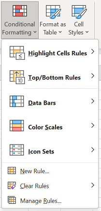
Click Home > Conditional Formatting > Highlight Cells Rules > Duplicate Values.

-
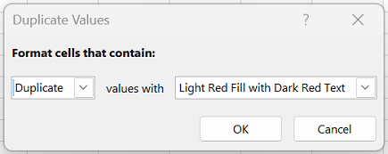
In the box next to values with, pick the formatting you want to apply to the duplicate values, and then click OK.
Remove duplicate values
When you use the Remove Duplicates feature, the duplicate data will be permanently deleted. Before you delete the duplicates, it’s a good idea to copy the original data to another worksheet so you don’t accidentally lose any information.
-
Select the range of cells that has duplicate values you want to remove.
-
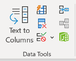
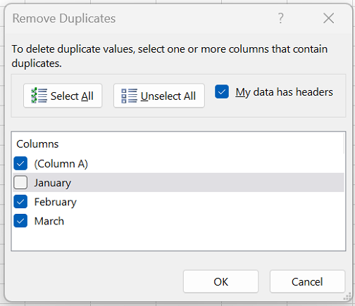
Click Data > Remove Duplicates, and then Under Columns, check or uncheck the columns where you want to remove the duplicates.
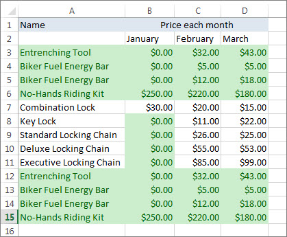
For example, in this worksheet, the January column has price information I want to keep.
So, I unchecked January in the Remove Duplicates box.
-
Click OK.
Note: The counts of duplicate and unique values given after removal may include empty cells, spaces, etc.
Need more help?

Need more help?
Duplicate values in your data can be a big problem! It can lead to substantial errors and over estimate your results.
But finding and removing them from your data is actually quite easy in Excel.
In this tutorial, we are going to look at 7 different methods to locate and remove duplicate values from your data.
Video Tutorial
What Is A Duplicate Value?
Duplicate values happen when the same value or set of values appear in your data.
For a given set of data you can define duplicates in many different ways.
In the above example, there is a simple set of data with 3 columns for the Make, Model and Year for a list of cars.
- The first image highlights all the duplicates based only on the Make of the car.
- The second image highlights all the duplicates based on the Make and Model of the car. This results in one less duplicate.
- The second image highlights all the duplicates based on all columns in the table. This results in even less values being considered duplicates.
The results from duplicates based on a single column vs the entire table can be very different. You should always be aware which version you want and what Excel is doing.
Find And Remove Duplicate Values With The Remove Duplicates Command
Removing duplicate values in data is a very common task. It’s so common, there’s a dedicated command to do it in the ribbon.
Select a cell inside the data which you want to remove duplicates from and go to the Data tab and click on the Remove Duplicates command.
Excel will then select the entire set of data and open up the Remove Duplicates window.
- You then need to tell Excel if the data contains column headers in the first row. If this is checked, then the first row of data will be excluded when finding and removing duplicate values.
- You can then select which columns to use to determine duplicates. There are also handy Select All and Unselect All buttons above you can use if you’ve got a long list of columns in your data.
When you press OK, Excel will then remove all the duplicate values it finds and give you a summary count of how many values were removed and how many values remain.
This command will alter your data so it’s best to perform the command on a copy of your data to retain the original data intact.
Find And Remove Duplicate Values With Advanced Filters
There is also another way to get rid of any duplicate values in your data from the ribbon. This is possible from the advanced filters.
Select a cell inside the data and go to the Data tab and click on the Advanced filter command.
This will open up the Advanced Filter window.
- You can choose to either to Filter the list in place or Copy to another location. Filtering the list in place will hide rows containing any duplicates while copying to another location will create a copy of the data.
- Excel will guess the range of data, but you can adjust it in the List range. The Criteria range can be left blank and the Copy to field will need to be filled if the Copy to another location option was chosen.
- Check the box for Unique records only.
Press OK and you will eliminate the duplicate values.
Advanced filters can be a handy option for getting rid of your duplicate values and creating a copy of your data at the same time. But advanced filters will only be able to perform this on the entire table.
Find And Remove Duplicate Values With A Pivot Table
Pivot tables are just for analyzing your data, right?
You can actually use them to remove duplicate data as well!
You won’t actually be removing duplicate values from your data with this method, you will be using a pivot table to display only the unique values from the data set.
First, create a pivot table based on your data. Select a cell inside your data or the entire range of data ➜ go to the Insert tab ➜ select PivotTable ➜ press OK in the Create PivotTable dialog box.
With the new blank pivot table add all fields into the Rows area of the pivot table.
You will then need to change the layout of the resulting pivot table so it’s in a tabular format. With the pivot table selected, go to the Design tab and select Report Layout. There are two options you will need to change here.
- Select the Show in Tabular Form option.
- Select the Repeat All Item Labels option.
You will also need to remove any subtotals from the pivot table. Go to the Design tab ➜ select Subtotals ➜ select Do Not Show Subtotals.
You now have a pivot table that mimics a tabular set of data!
Pivot tables only list unique values for items in the Rows area, so this pivot table will automatically remove any duplicates in your data.
Find And Remove Duplicate Values With Power Query
Power Query is all about data transformation, so you can be sure it has the ability to find and remove duplicate values.
Select the table of values which you want to remove duplicates from ➜ go to the Data tab ➜ choose a From Table/Range query.
Remove Duplicates Based On One Or More Columns
With Power Query, you can remove duplicates based on one or more columns in the table.
You need to select which columns to remove duplicates based on. You can hold Ctrl to select multiple columns.
Right click on the selected column heading and choose Remove Duplicates from the menu.
You can also access this command from the Home tab ➜ Remove Rows ➜ Remove Duplicates.
= Table.Distinct(#"Previous Step", {"Make", "Model"})If you look at the formula that’s created, it is using the Table.Distinct function with the second parameter referencing which columns to use.
Remove Duplicates Based On The Entire Table
To remove duplicates based on the entire table, you could select all the columns in the table then remove duplicates. But there is a faster method that doesn’t require selecting all the columns.
There is a button in the top left corner of the data preview with a selection of commands that can be applied to the entire table.
Click on the table button in the top left corner ➜ then choose Remove Duplicates.
= Table.Distinct(#"Previous Step")If you look at the formula that’s created, it uses the same Table.Distinct function with no second parameter. Without the second parameter, the function will act on the whole table.
Keep Duplicates Based On A Single Column Or On The Entire Table
In Power Query, there are also commands for keeping duplicates for selected columns or for the entire table.
Follow the same steps as removing duplicates, but use the Keep Rows ➜ Keep Duplicates command instead. This will show you all the data that has a duplicate value.
Find And Remove Duplicate Values Using A Formula
You can use a formula to help you find duplicate values in your data.
First you will need to add a helper column that combines the data from any columns which you want to base your duplicate definition on.
= [@Make] & [@Model] & [@Year]The above formula will concatenate all three columns into a single column. It uses the ampersand operator to join each column.
= TEXTJOIN("", FALSE , CarList[@[Make]:[Year]])If you have a long list of columns to combine, you can use the above formula instead. This way you can simply reference all the columns as a single range.
You will then need to add another column to count the duplicate values. This will be used later to filter out rows of data that appear more than once.
= COUNTIFS($E$3:E3, E3)Copy the above formula down the column and it will count the number of times the current value appears in the list of values above.
If the count is 1 then it’s the first time the value is appearing in the data and you will keep this in your set of unique values. If the count is 2 or more then the value has already appeared in the data and it is a duplicate value which can be removed.
Add filters to your data list.
- Go to the Data tab and select the Filter command.
- Use the keyboard shortcut Ctrl + Shift + L.
Now you can filter on the Count column. Filtering on 1 will produce all the unique values and remove any duplicates.
You can then select the visible cells from the resulting filter to copy and paste elsewhere. Use the keyboard shortcut Alt + ; to select only the visible cells.
Find And Remove Duplicate Values With Conditional Formatting
With conditional formatting, there’s a way to highlight duplicate values in your data.
Just like the formula method, you need to add a helper column that combines the data from columns. The conditional formatting doesn’t work with data across rows, so you’ll need this combined column if you want to detect duplicates based on more than one column.
Then you need to select the column of combined data.
To create the conditional formatting, go to the Home tab ➜ select Conditional Formatting ➜ Highlight Cells Rules ➜ Duplicate Values.
This will open up the conditional formatting Duplicate Values window.
- You can select to either highlight Duplicate or Unique values.
- You can also choose from a selection of predefined cell formats to highlight the values or create your own custom format.
Warning: The previous methods to find and remove duplicates considers the first occurrence of a value as a duplicate and will leave it intact. However, this method will highlight the first occurrence and will not make any distinction.
With the values highlighted, you can now filter on either the duplicate or unique values with the filter by color option. Make sure to add filters to your data. Go to the Data tab and select the Filter command or use the keyboard shortcut Ctrl + Shift + L.
- Click on the filter toggle.
- Select Filter by Color in the menu.
- Filter on the color used in the conditional formatting to select duplicate values or filter on No Fill to select unique values.
You can then select just the visible cells with the keyboard shortcut Alt + ;.
Find And Remove Duplicate Values Using VBA
There is a built in command in VBA for removing duplicates within list objects.
Sub RemoveDuplicates()Dim DuplicateValues As RangeSet DuplicateValues = ActiveSheet.ListObjects("CarList").RangeDuplicateValues.RemoveDuplicates Columns:=Array(1, 2, 3), Header:=xlYesEnd Sub
The above procedure will remove duplicates from an Excel table named CarList.
Columns:=Array(1, 2, 3)The above part of the procedure will set which columns to base duplicate detection on. In this case it will be on the entire table since all three columns are listed.
Header:=xlYesThe above part of the procedure tells Excel the first row in our list contains column headings.
You will want to create a copy of your data before running this VBA code, as it can’t be undone after the code runs.
Conclusions
Duplicate values in your data can be a big obstacle to a clean data set.
Thankfully, there are many options in Excel to easily remove those pesky duplicate values.
So, what’s your go to method to remove duplicates?
About the Author
John is a Microsoft MVP and qualified actuary with over 15 years of experience. He has worked in a variety of industries, including insurance, ad tech, and most recently Power Platform consulting. He is a keen problem solver and has a passion for using technology to make businesses more efficient.
This wikiHow teaches you how to remove duplicate entries from a Microsoft Excel spreadsheet.
-
1
Double-click your Excel document. This will open the spreadsheet in Excel.
- You can also open an existing document from the «Recent» section of the Open tab.
-
2
Select your data group. To do so, click the top entry, hold down ⇧ Shift, and click the bottom entry.
- If you’re selecting multiple columns, click the top-left entry, then click the bottom-right entry while holding down ⇧ Shift.
-
3
Click the Data tab. It’s a tab on the left side of the green ribbon at the top of the Excel window.
-
4
Click Remove Duplicates. This option is the «Data Tools» section of the Data toolbar near the top of the Excel window. A pop-up window will appear with the option of selecting or de-selecting columns.
-
5
Make sure each column you wish to edit is selected. You’ll see several column names (e.g., «Column A», «Column B») next to checkboxes; clicking a checkbox will de-select the column in question.
- By default, all columns next to the one you select will be listed and checked here.
- You can click Select All to select all of the columns listed.
-
6
Click OK. Doing so will remove any duplicates from your Excel spreadsheet selection.
- If no duplicates are reported when you know there are duplicates, try selecting one column at a time.


-
1
Double-click your Excel document. This will open the spreadsheet in Excel, allowing you to check it for cells containing duplicate values by using the Conditional Formatting feature. If you want to look for duplicates but don’t want to delete them by default, this is a good way of doing so.
- You can also open an existing document from the «Recent» section of the Open tab.
-
2
Click the top-left cell in your data group. Doing so will select it.
- Exclude headers (e.g., «Date», «Time», etc.) from your selection.
- If you’re just selecting one row, click the left-most entry.
- If you’re just selecting one column, click the top-most entry.
-
3
Hold down ⇧ Shift and click the bottom-right cell. This will select any data between the top-left corner and the bottom-right corner of the data group.
- If you’re selecting one row, just click the right-most cell with data in it.
- If you’re selecting one column, just click the bottom-most entry with data in it.
-
4
Click Conditional Formatting. It’s in the «Styles» section of the Home tab. Doing so will prompt a drop-down menu.
- You may first need to click Home near the top of the Excel window to view this option.
-
5
Select Highlight Cells Rules. You’ll see a window pop out from here.
-
6
Click Duplicate Values. It’s at the bottom of the pop-out menu. Clicking this option will select all duplicate values in your selected range.


Ask a Question
200 characters left
Include your email address to get a message when this question is answered.
Submit
About this article
Article SummaryX
1. Open the Excel document.
2. Select your data group.
3. Click Data.
4. Click Remove Duplicates.
5. Click OK.
Did this summary help you?
Thanks to all authors for creating a page that has been read 420,580 times.
Reader Success Stories
-

«Simple click that save me tons of time sorting and filtering.»
Is this article up to date?
Excel spreadsheets continue to represent a key tool for data storage and visualization. Functionalities such as Find & Replace or Sort help users speed up repetitive tasks that would otherwise be time-consuming and inefficient. Just like working on a spreadsheet with blank rows or cells that interfere with the correct application of rules and formulae, duplicate data can cause similar issues.
In this post, you will learn different ways to find duplicate values to either highlight this information or delete as many duplicates as needed. From more basic highlighting features to more advanced filtering options, you’ll learn how to work with the full potential of the desktop version of Excel.
If you want to avoid duplicate data entry in Google Sheets, you can do that easily using Layer. Layer is a free add-on that allows you to share sheets or ranges of your main spreadsheet with different people. On top of that, you get to monitor and approve edits and changes made to the shared files before they’re merged back into your master file, giving you more control over your data.
Install the Layer Google Sheets Add-On today and Get Free Access to all the paid features, so you can start managing, automating, and scaling your processes on top of Google Sheets!
How to find and remove duplicate rows in Excel?
The various methods shown in this article will first find the duplicate values to be removed and then show how to delete them. This two-step process is crucial, especially considering that you may not want to delete the duplicates automatically and keep only the unique value. Let’s look at the first method to remove all duplicates.
How to Check for Duplicates in Excel?
How to remove duplicates using the Remove Duplicates feature?
What is the shortcut to removing duplicates in Excel? The shortcut is actually a built-in command available in the ribbon, which you can use in the following way.
- 1. Open your Excel spreadsheet and select any range in your spreadsheet which you want to delete duplicate rows from.

How to Find and Remove Duplicates in Excel — Find duplicate rows
- 2. Go to Data > Remove duplicates.

How to Find and Remove Duplicates in Excel — Remove duplicates
If you haven’t selected all data in your spreadsheet, Excel will give you the option of expanding the search to the entire document, which is recommended. Click “OK”.
- 3. In case your data selection has headers, tick the column boxes that contain them so as not to be counted in the duplicate search. All columns in my example contain headers, so I’ll leave all boxes ticked. Click “OK”.

How to Find and Remove Duplicates in Excel — Remove headers from duplicate search
- 4. Excel prompts you with a dialog box informing you about the exact number of duplicate values it found and removed, as well as the number of unique values remaining in your spreadsheet.

How to Find and Remove Duplicates in Excel — Duplicate values found
How to Combine Multiple Excel Columns Into One?
There are many ways to combine multiple columns into a single column in Excel. Here’s how to do it without losing any data
READ MORE

How to delete duplicates in Excel but keep one?
Although the previous method is helpful at targeting all duplicates, this means that the unique data will also be permanently deleted. To avoid this, you may want to explore the following methods.
Here’s how to delete duplicates in Excel but keep one; we strongly recommend that you always keep a copy spreadsheet in case you want to go back to the original dataset.
How to remove duplicates using the Advanced Filter option?
This is a straightforward way to get rid of any duplicate content without deleting them entirely; instead, the Advanced filter option hides your duplicates from your dataset.
- 1. Select a cell in your dataset and go to Data > Advanced filter to the far right.

How to Find and Remove Duplicates in Excel — Advanced filter
- 2. Choose to “Filter the list, in-place” or “Copy to another location”. The first option will hide any row containing duplicates, while the second will make a copy of the data.

How to Find and Remove Duplicates in Excel — Filter list
Leave the “List range” field empty, if you want Excel to list it automatically. You can also leave the “Criteria range” empty. The only mandatory field to fill out is the “Copy to” if you selected the “Copy to another location” option.
- 3. Tick the “Unique records only” box to keep the unique values, and then “OK” to remove all duplicates.

How to Find and Remove Duplicates in Excel — How to keep unique values
Advanced filters are an excellent way to remove duplicate values while keeping a copy of the original data. Don’t forget that the Advanced filter option only applies to the entire table.
How to remove duplicates using Excel formulae?
Although you can combine various formulae to remove duplicates in Excel, in 2018, Microsoft integrated the UNIQUE formula to make this process much easier. First, let’s explore the syntax of the UNIQUE formula:
=UNIQUE (array, [by_col], [exactly_once])
- array refers to the range of cells we will extract unique values from and represents the only required argument.
- [by_col] is an optional parameter determining the search for unique values by rows or columns.
- [exactly_once] is the other optional parameter and sets the behavior for values that appear more than once. If you want the formula to return items that appear exactly once, then write “TRUE”; however, if you want it to return every distinct item, then write “FALSE”.
Let’s now apply the =UNIQUE formula to our dataset.
- 1. Enter the formula next to the set of data. You can either leave one column in between or place it directly next to the last data column. Like in most Excel formulae, as soon as you type at the beginning of the formula, the rest will prompt automatically. Select the range you want to apply the formula to.

How to Find and Remove Duplicates in Excel — UNIQUE formula
- 2. You can leave the second parameter [by_col] by simply including the comma before and after its place. Let’s first see what happens when we include “TRUE” for the [exactly_once] parameter.

How to Find and Remove Duplicates in Excel — UNIQUE function
- 3. As soon as you press the Return key, Excel removes all duplicates. In this example, it has removed rows 5 and 6.

How to Find and Remove Duplicates in Excel — TRUE UNIQUE formula
Let’s see how by including “FALSE” as the last parameter, Excel will keep the unique value.
- 1. Follow the previous steps, and now wrote “FALSE”, to return every distinct value.

How to Find and Remove Duplicates in Excel — FALSE UNIQUE formula
- 2. Now, the UNIQUE formula has returned row 5 and only deleted the duplicate value in row 6.

How to Find and Remove Duplicates in Excel — FALSE UNIQUE formula return
How to remove duplicates using conditional formatting?
Conditional formatting is an Excel feature that helps users filter, sort, and organize data according to built-in rules or custom ones created by the user. The most common feature is the “Highlight Cell Rules”, which allows you to format cell values according to color, font, and various other format styles. Although this method won’t directly remove duplicates, it will make them extremely clear to identify.
- 1. Select the range of cells you want to apply the conditional formatting rule to. Then go to Home > Conditional Formatting > Highlight Cell Rules > Duplicate Values.

How to Find and Remove Duplicates in Excel — Conditional formatting
- 2. Set the “Style” to “Classic” and then “Format only unique or duplicate values”. Don’t forget to leave the drop-down menu to “duplicate”. Finally, choose the formatting style using the “Format with” drop-down menu. Click “OK”.

How to Find and Remove Duplicates in Excel — Conditional formatting remove duplicates
- 3. You can see how Excel highlights all duplicate values, including the cells. This means that you will need to make sure to only remove rows unless you are actually interested in removing all duplicates.

How to Find and Remove Duplicates in Excel — Highlight duplicates conditional formatting]
In case you want to highlight rows, you can combine all row values in one cell using the =CONCAT formula; if you would like to learn more about this function, read this article on the Microsoft support page.
How to remove duplicates based on one or more columns in Excel?
As a more advanced use of Excel, you can remove duplicates based on one or more columns using Power Query. This feature allows you to select the columns you would like to remove the duplicates from. Let’s explore how to use Power Query to remove duplicates based on one or more columns.
- 1. Go to Data > Get Data (Power Query).

How to Find and Remove Duplicates in Excel — Power Query
- 2. Choose “Excel workbook” as your data source.
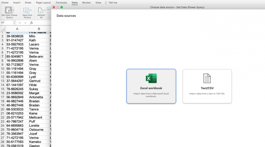
How to Find and Remove Duplicates in Excel — Power Query data source
- 3. Browse through your files and select the spreadsheet you want to apply the Power Query function to. Click “Next”.

How to Find and Remove Duplicates in Excel — Power Query load data
- 4. Tick the checkbox next to the worksheet containing your data (located in the left-side menu). Then, click “Load” in the bottom right-hand corner.

How to Find and Remove Duplicates in Excel — Power Query load data
- 5. As you can see, the dataset has been transformed into a table.

How to Find and Remove Duplicates in Excel — Power Query table
- 6. Select the columns to apply the Power Query to by pressing Ctrl/Cmd + click on the columns.

How to Find and Remove Duplicates in Excel — Power Query table
- 7. To delete duplicates, simply click on “Remove Duplicates” in the “Data” tab. Then click “OK” in the pop-up dialog box.

How to Find and Remove Duplicates in Excel — Remove Duplicates
- 8. Excel will inform you about the number of duplicates removed and how many unique values remain.

How to Find and Remove Duplicates in Excel — Final Alert message
Don’t worry about removing all duplicates, since the dataset you worked on is a copy created by the Power Query function. However, if you want to keep unique values, follow the steps outlined in the sections on the Advanced Filter option or =UNIQUE formula in Excel.
Want to Boost Your Team’s Productivity and Efficiency?
Transform the way your team collaborates with Confluence, a remote-friendly workspace designed to bring knowledge and collaboration together. Say goodbye to scattered information and disjointed communication, and embrace a platform that empowers your team to accomplish more, together.
Key Features and Benefits:
- Centralized Knowledge: Access your team’s collective wisdom with ease.
- Collaborative Workspace: Foster engagement with flexible project tools.
- Seamless Communication: Connect your entire organization effortlessly.
- Preserve Ideas: Capture insights without losing them in chats or notifications.
- Comprehensive Platform: Manage all content in one organized location.
- Open Teamwork: Empower employees to contribute, share, and grow.
- Superior Integrations: Sync with tools like Slack, Jira, Trello, and more.
Limited-Time Offer: Sign up for Confluence today and claim your forever-free plan, revolutionizing your team’s collaboration experience.
Conclusion
As we have seen, there are many ways to identify and eliminate duplicates in your data, depending on your needs. Not only can you now successfully organize your data correctly, but removing duplicates makes it easier to identify key patterns and create accurate reports, particularly when working with larger datasets.
Содержание
- Как удалить дубликаты в Excel
- Удалить дубликаты строк в Excel с помощью функции «Удалить дубликаты»
- Удалить дубликаты в Excel – Функция Удалить дубликаты в Excel
- Удалить дубликаты в Excel – Выбор столбца(ов), который вы хотите проверить на наличие дубликатов
- Удалить дубликаты в Excel – Сообщение о том, сколько было удалено дубликатов
- Удалить дубликаты, скопировав уникальные записи в другое место
- Удалить дубликаты в Excel – Использование дополнительного фильтра для удаления дубликатов
- Удалить дубликаты в Excel – Фильтр дубликатов
- Удалить дубликаты в Excel – Уникальные записи, скопированные из другого места
- Удаление дубликатов в Microsoft Excel
- Команда Удалить дубликаты в Excel
- Поиск и выделение дубликатов цветом в Excel
- Поиск и выделение дубликатов цветом в одном столбце в Эксель
- Поиск и выделение дубликатов цветом в нескольких столбцах в Эксель
- Поиск и выделение цветом дубликатов строк в Excel
- Удаление дублирующихся строк вручную
- Удаление повторений при помощи “умной таблицы”
- Использование фильтра
- Условное форматирование
- Формула для удаления повторяющихся строк
- Как в Эксель удалить повторяющиеся строки через «Расширенный фильтр»
- Как убрать дубли в Excel через функцию «Удалить дубликаты»
- Поиск одинаковых значений в Excel
- Ищем в таблицах Excel все повторяющиеся значения
- Удаление одинаковых значений из таблицы Excel
- Расширенный фильтр: оставляем только уникальные записи
- Поиск дублирующихся значений с помощью сводных таблиц
- Заключение
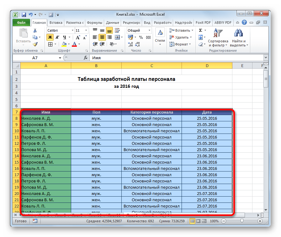
Ниже на рисунке изображена таблица с дублирующими значениями. Строка 3 содержит тоже значение, что и строка 6. А значение строки 4 = строке 7. Ячейки с числами в дублирующихся строках имеют одинаковые значения и разные форматы. У них отличается количество разрядов после запятой. Выполним 2 разные операции для удаления дубликатов.
Устранение дубликатов на основе значений колонки с текстом:
- Создайте умную таблицу (CTRL+T) с повторяющимися значениями как на рисунке:
- Щелкните по таблице и выберите инструмент «Работа с таблицами»-«Конструктор»-«Удалить дубликаты» в разделе инструментов «Сервис».
- В появившемся окне «Удалить дубликаты», следует отключить проверку по 4-му столбцу «Цена».


Строки 6 и 7 распознаны как дублирующие и удалены из таблицы. Если в пункте 2 не отключить проверку по столбцу ни одна строка не будет удалена, так как для Excel все числа в колонке «Цена» считаются разными.
Удалить дубликаты строк в Excel с помощью функции «Удалить дубликаты»
Если вы используете последними версиями Excel 2007, Excel 2010, Excel 2013 или Excel 2016, у вас есть преимущество, потому что эти версии содержат встроенную функцию для поиска и удаления дубликатов – функцию Удалить дубликаты.
Эта функция позволяет находить и удалять абсолютные дубликаты (ячейки или целые строки), а также частично соответствующие записи (строки, которые имеют одинаковые значения в указанном столбце или столбцах). Разберем на примере, как пошагово использовать функцию Удалить дубликаты в Excel.
Примечание. Поскольку функция Удалить дубликаты навсегда удаляет идентичные записи, рекомендуется создать копию исходных данных перед удалением повторяющихся строк.
- Для начала выберите диапазон, в котором вы хотите удалить дубликаты. Чтобы выбрать всю таблицу, нажмите Ctrl+A.
- Далее перейдите на вкладку «ДАННЫЕ» –> группа «Работа с данными» и нажмите кнопку «Удалить дубликаты».

Удалить дубликаты в Excel – Функция Удалить дубликаты в Excel
- Откроется диалоговое окно «Удалить дубликаты». Выберите столбцы для проверки дубликатов и нажмите «ОК».
- Чтобы удалить дубликаты строк, имеющие полностью одинаковые значения во всех столбцах, оставьте флажки рядом со всеми столбцами, как показано на изображении ниже.
- Чтобы удалить частичные дубликаты на основе одного или нескольких ключевых столбцов, выберите только соответствующие столбцы. Если в вашей таблице много столбцов, лучше сперва нажать кнопку «Снять выделение», а затем выбрать столбцы, которые вы хотите проверить на предмет дубликатов.
- Если в вашей таблице нет заголовков, уберите флаг с поля «Мои данные содержат заголовки» в правом верхнем углу диалогового окна, которое обычно выбирается по умолчанию.

Удалить дубликаты в Excel – Выбор столбца(ов), который вы хотите проверить на наличие дубликатов
Готово! Все дубликаты строк в выбранном диапазоне удалены, и отображается сообщение, указывающее, сколько было удалено дубликатов записей и сколько уникальных значений осталось.

Удалить дубликаты в Excel – Сообщение о том, сколько было удалено дубликатов
Функция Удалить дубликаты в Excel удаляет 2-ой и все последующие дубликаты экземпляров, оставляя все уникальные строки и первые экземпляры одинаковых записей. Если вы хотите удалить дубликаты строк, включая первые вхождения, т.е. если вы ходите удалить все дублирующие ячейки. Или в другом случае, если есть два или более дубликата строк, и первый из них вы хотите оставить, а все последующие дубликаты удалить, то используйте одно из следующих решений описанных в этом разделе.
Удалить дубликаты, скопировав уникальные записи в другое место
Другой способ удалить дубликаты в Excel – это разделение уникальных значений и копирование их на другой лист или в выбранный диапазон на текущем листе. Разберем этот способ.
- Выберите диапазон или всю таблицу, которую вы хотите удалить дубликаты.
- Перейдите во вкладку «ДАННЫЕ» –> группа «Сортировка и фильтр» и нажмите кнопку «Дополнительно».

Удалить дубликаты в Excel – Использование дополнительного фильтра для удаления дубликатов
- В диалоговом окне «Расширенный фильтр» выполните следующие действия:
- Выберите пункт «скопировать результат в другое место».
- Проверьте, отображается ли правильный диапазон в Исходном диапазоне. Это должен быть диапазон, выбранный на шаге 1.
- В поле Поместить результат в диапазон введите диапазон, в котором вы хотите скопировать уникальные значения (на самом деле достаточно выбрать верхнюю левую ячейку диапазона назначения).
- Выберите Только уникальные записи

Удалить дубликаты в Excel – Фильтр дубликатов
- Наконец, нажмите «ОК». Excel удалит дубликаты и скопирует уникальные значения в новое указанное место:

Удалить дубликаты в Excel – Уникальные записи, скопированные из другого места
Таким образом вы получаете новые данные, на основе указанных, но с удаленными дубликатами.
Обратите внимание, что расширенный фильтр позволяет копировать отфильтрованные значения в другое место только на активном листе.
Удаление дубликатов в Microsoft Excel
Для меня человека который проводит время в отпуске и работает с мобильного интернета скорость которого измеряется от 1-2 мегабита, прокачивать в пустую такое кол-во товара с фотографиями смысла не имеет и время пустое и трафика сожрет не мало, поэтому решил повторяющиеся товары просто удалить и тут столкнулся с тем, что удалить дублирующиеся значения в столбце не так то и просто, потому как стандартная функция excel 2010 делает это топорно и после удаления дубликата двигает вверх нижние значения и в итоге у нас все перепутается в документе и будет каша.
Команда Удалить дубликаты в Excel
Microsoft Excel располагает встроенным инструментом, который позволяет находить и удалять дубликаты строк. Начнем с поиска повторяющихся строк. Для этого выберите любую ячейку в таблице, а затем выделите всю таблицу, нажав Ctrl+A.

Перейдите на вкладку Date (Данные), а затем нажмите команду Remove Duplicates (Удалить дубликаты), как показано ниже.

Появится небольшое диалоговое окно Remove Duplicates (Удалить дубликаты). Можно заметить, что выделение первой строки снимается автоматически. Причиной тому является флажок, установленный в пункте My data has headers (Мои данные содержат заголовки).

В нашем примере нет заголовков, поскольку таблица начинается с 1-й строки. Поэтому снимем флажок. Сделав это, Вы заметите, что вся таблица снова выделена, а раздел Columns (Колонны) изменится с dulpicate на Column A, B и С.

Теперь, когда выделена вся таблица, нажмите OK, чтобы удалить дубликаты. В нашем случае все строки с повторяющимися данными удалятся, за исключением одной. Вся информация об удалении отобразится во всплывающем диалоговом окне.

Поиск и выделение дубликатов цветом в Excel
Дубликаты в таблицах могу встречаться в разных формах. Это могут быть повторяющиеся значения в одной колонке и в нескольких, а также в одной или нескольких строках.
Поиск и выделение дубликатов цветом в одном столбце в Эксель
Самый простой способ найти и выделить цветом дубликаты в Excel, это использовать условное форматирование.
Как это сделать:
- Выделим область с данными, в которой нам нужно найти дубликаты:

- На вкладке “Главная” на Панели инструментов нажимаем на пункт меню “Условное форматирование” -> “Правила выделения ячеек” -> “Повторяющиеся значения”:

- Во всплывающем диалоговом окне выберите в левом выпадающем списке пункт “Повторяющиеся”, в правом выпадающем списке выберите каким цветом будут выделены дублирующие значения. Нажмите кнопку “ОК”:

- После этого, в выделенной колонке, будут подсвечены цветом дубликаты:

Подсказка: не забудьте проверить данные вашей таблицы на наличие лишних пробелов. Для этого лучше использовать функцию TRIM (СЖПРОБЕЛЫ).
Поиск и выделение дубликатов цветом в нескольких столбцах в Эксель
Если вам нужно вычислить дубликаты в нескольких столбцах, то процесс по их вычислению такой же как в описанном выше примере. Единственное отличие, что для этого вам нужно выделить уже не одну колонку, а несколько:
- Выделите колонки с данными, в которых нужно найти дубликаты;
- На вкладке “Главная” на Панели инструментов нажимаем на пункт меню “Условное форматирование” -> “Правила выделения ячеек” -> “Повторяющиеся значения”;
- Во всплывающем диалоговом окне выберите в левом выпадающем списке пункт “Повторяющиеся”, в правом выпадающем списке выберите каким цветом будут выделены повторяющиеся значения. Нажмите кнопку “ОК”:
- После этого в выделенной колонке будут подсвечены цветом дубликаты:
Поиск и выделение цветом дубликатов строк в Excel
Поиск дубликатов повторяющихся ячеек и целых строк с данными это разные понятия. Обратите внимание на две таблицы ниже:


В таблицах выше размещены одинаковые данные. Их отличие в том, что на примере слева мы искали дубликаты ячеек, а справа мы нашли целые повторяющие строчки с данными.
Рассмотрим как найти дубликаты строк:
- Справа от таблицы с данными создадим вспомогательный столбец, в котором напротив каждой строки с данными проставим формулу, объединяющую все значения строки таблицы в одну ячейку:
=A2&B2&C2&D2
Во вспомогательной колонке вы увидите объединенные данные таблицы:

Теперь, для определения повторяющихся строк в таблице сделайте следующие шаги:
- Выделите область с данными во вспомогательной колонке (в нашем примере это диапазон ячеек E2:E15
- На вкладке “Главная” на Панели инструментов нажимаем на пункт меню “Условное форматирование” -> “Правила выделения ячеек” -> “Повторяющиеся значения”;
- Во всплывающем диалоговом окне выберите в левом выпадающем списке “Повторяющиеся”, в правом выпадающем списке выберите каким цветом будут выделены повторяющиеся значения. Нажмите кнопку “ОК”:
- После этого в выделенной колонке будут подсвечены дублирующиеся строки:

На примере выше, мы выделили строки в созданной вспомогательной колонке.
Но что, если нам нужно выделить цветом строки не во вспомогательном столбце, а сами строки в таблице с данными?
Для этого давайте сделаем следующее:
- Также как и в примере выше создадим вспомогательный столбец, в каждой строке которого проставим следующую формулу:
=A2&B2&C2&D2
Таким образом, мы получим в одной ячейке собранные данные всей строки таблицы:
- Теперь, выделим все данные таблицы (за исключением вспомогательного столбца). В нашем случае это ячейки диапазона A2:D15
- Затем, на вкладке “Главная” на Панели инструментов нажмем на пункт “Условное форматирование” -> “Создать правило”:

- В диалоговом окне “Создание правила форматирования” кликните на пункт “Использовать формулу для определения форматируемых ячеек” и в поле “Форматировать значения, для которых следующая формула является истинной” вставьте формулу:
=СЧЁТЕСЛИ($E$2:$E$15;$E2)>1

- Не забудьте задать формат найденных дублированных строк.
Эта формула проверяет диапазон данных во вспомогательной колонке и при наличии повторяющихся строк выделяет их цветом в таблице:

Удаление дублирующихся строк вручную
Первый метод максимально прост и предполагает удаление дублированных строк при помощи специального инструмента на ленте вкладки “Данные”.
- Полностью выделяем все ячейки таблицы с данными, воспользовавшись, например, зажатой левой кнопкой мыши.
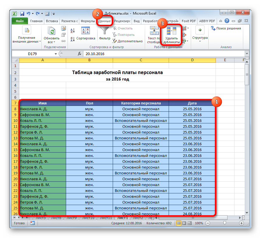
- Во вкладке “Данные” в разделе инструментов “Работа с данными” находим кнопку “Удалить дубликаты” и кликаем на нее.

- Переходим к настройкам параметров удаления дубликатов:
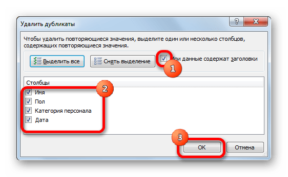
- Если обрабатываемая таблица содержит шапку, то проверяем пункт “Мои данные содержат заголовки” – он должен быть отмечен галочкой.
- Ниже, в основном окне, перечислены названия столбцов, по которым будет осуществляться поиск дубликатов. Система считает совпадением ситуацию, в которой в строках повторяются значения всех выбранных в настройке столбцов. Если убрать часть столбцов из сравнения, повышается вероятность увеличения количества похожих строк.
- Тщательно все проверяем и нажимаем ОК.

- Далее программа Эксель в автоматическом режиме найдет и удалит все дублированные строки.
- По окончании процедуры на экране появится соответствующее сообщение с информацией о количестве найденных и удаленных дубликатов, а также о количестве оставшихся уникальных строк. Для закрытия окна и завершения работы данной функции нажимаем кнопку OK.


Удаление повторений при помощи “умной таблицы”
Еще один способ удаления повторяющихся строк – использование “умной таблицы“. Давайте рассмотрим алгоритм пошагово.
- Для начала, нам нужно выделить всю таблицу, как в первом шаге предыдущего раздела.

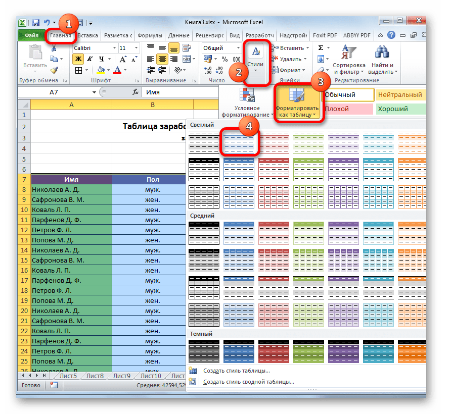
- Во вкладке “Главная” находим кнопку “Форматировать как таблицу” (раздел инструментов “Стили“). Кликаем на стрелку вниз справа от названия кнопки и выбираем понравившуюся цветовую схему таблицы.

- После выбора стиля откроется окно настроек, в котором указывается диапазон для создания “умной таблицы“. Так как ячейки были выделены заранее, то следует просто убедиться, что в окошке указаны верные данные. Если это не так, то вносим исправления, проверяем, чтобы пункт “Таблица с заголовками” был отмечен галочкой и нажимаем ОК. На этом процесс создания “умной таблицы” завершен.

- Далее приступаем к основной задаче – нахождению задвоенных строк в таблице. Для этого:
- ставим курсор на произвольную ячейку таблицы;
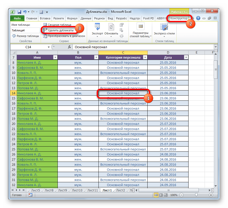
- переключаемся во вкладку “Конструктор” (если после создания “умной таблицы” переход не был осуществлен автоматически);
- в разделе “Инструменты” жмем кнопку “Удалить дубликаты“.
- Следующие шаги полностью совпадают с описанными в методе выше действиями по удалению дублированных строк.


Примечание: Из всех описываемых в данной статье методов этот является наиболее гибким и универсальным, позволяя комфортно работать с таблицами различной структуры и объема.
Использование фильтра
Следующий метод не удаляет повторяющиеся строки физически, но позволяет настроить режим отображения таблицы таким образом, чтобы при просмотре они скрывались.
- Как обычно, выделяем все ячейки таблицы.
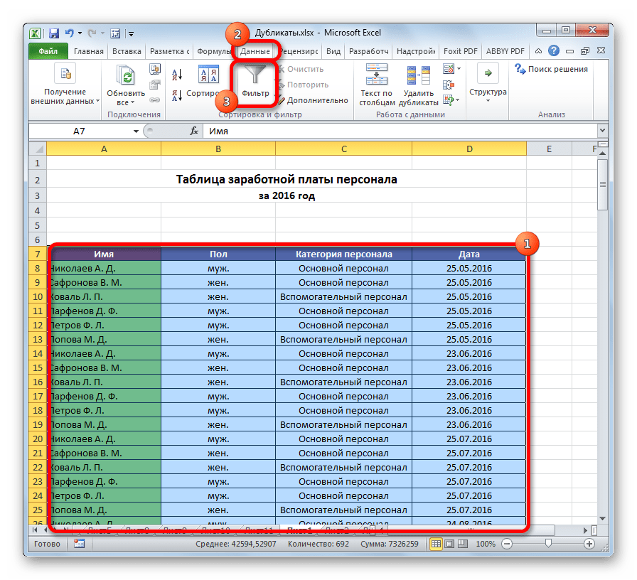
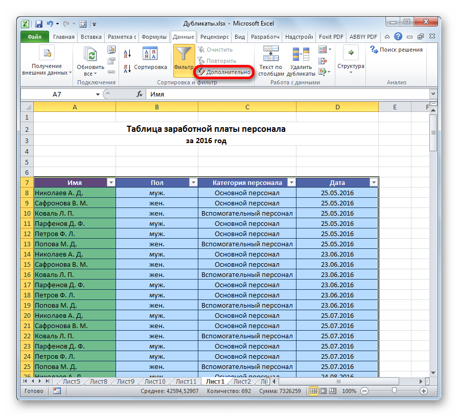
- Во вкладке “Данные” в разделе инструментов “Сортировка и фильтр” ищем кнопку “Фильтр” (иконка напоминает воронку) и кликаем на нее.
- После этого в строке с названиями столбцов таблицы появятся значки перевернутых треугольников (это значит, что фильтр включен). Чтобы перейти к расширенным настройкам, жмем кнопку “Дополнительно“, расположенную справа от кнопки “Фильтр“.
- В появившемся окне с расширенными настройками:
- как и в предыдущем способе, проверяем адрес диапазон ячеек таблицы;
- отмечаем галочкой пункт “Только уникальные записи“;
- жмем ОК.

- После этого все задвоенные данные перестанут отображаться в таблицей. Чтобы вернуться в стандартный режим, достаточно снова нажать на кнопку “Фильтр” во вкладке “Данные”.


Условное форматирование
Условное форматирование – гибкий и мощный инструмент, используемый для решения широкого спектра задач в Excel. В этом примере мы будем использовать его для выбора задвоенных строк, после чего их можно удалить любым удобным способом.
- Выделяем все ячейки нашей таблицы.
- Во вкладке “Главная” кликаем по кнопке “Условное форматирование“, которая находится в разделе инструментов “Стили“.
- Откроется перечень, в котором выбираем группу “Правила выделения ячеек“, а внутри нее – пункт “Повторяющиеся значения“.

- Окно настроек форматирования оставляем без изменений. Единственный его параметр, который можно поменять в соответствии с собственными цветовыми предпочтениями – это используемая для заливки выделяемых строк цветовая схема. По готовности нажимаем кнопку ОК.

- Теперь все повторяющиеся ячейки в таблице “подсвечены”, и с ними можно работать – редактировать содержимое или удалить строки целиком любым удобным способом.


Важно! Этом метод не настолько универсален, как описанные выше, так как выделяет все ячейки с одинаковыми значениями, а не только те, для которых совпадает вся строка целиком. Это видно на предыдущем скриншоте, когда нужные задвоения по названиям регионов были выделены, но вместе с ними отмечены и все ячейки с категориями регионов, потому что значения этих категорий повторяются.
Формула для удаления повторяющихся строк
Последний метод достаточно сложен, и им мало, кто пользуется, так как здесь предполагается использование сложной формулы, объединяющей в себе несколько простых функций. И чтобы настроить формулу для собственной таблицы с данными, нужен определенный опыт и навыки работы в Эксель.
Формула, позволяющая искать пересечения в пределах конкретного столбца в общем виде выглядит так:
Давайте посмотрим, как с ней работать на примере нашей таблицы:
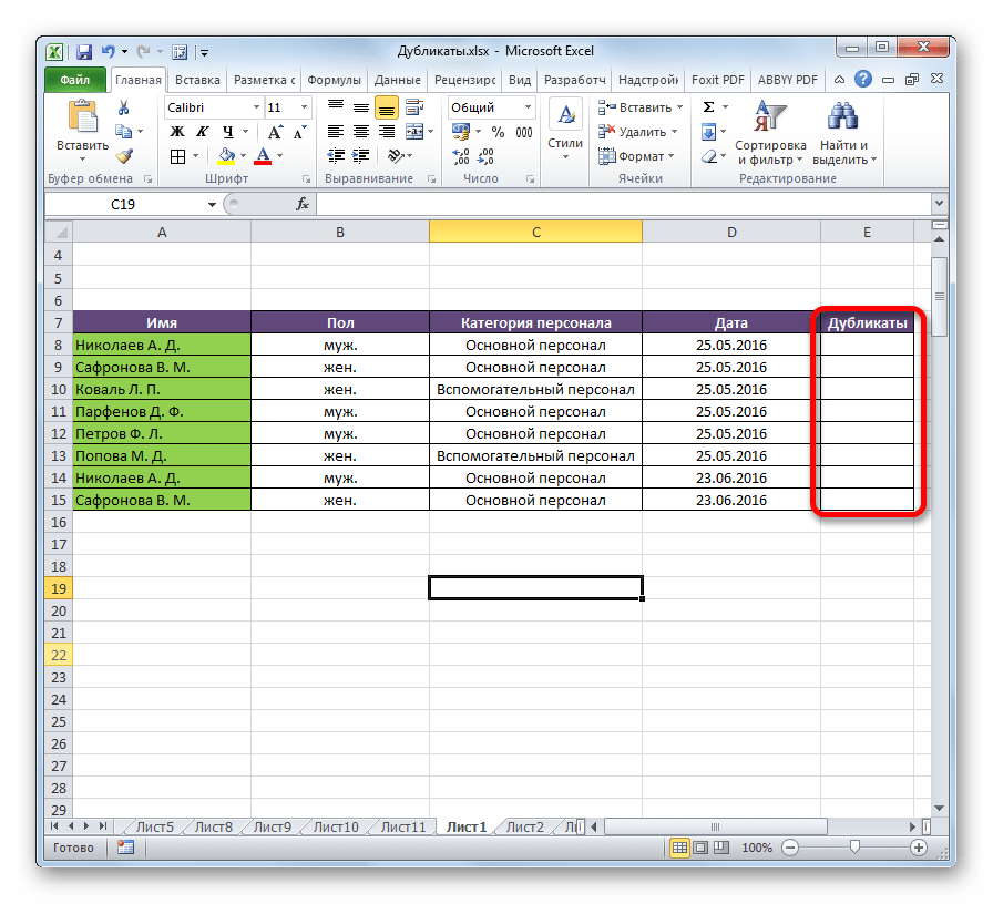
- Добавляем в конце таблицы новый столбец, специально предназначенный для отображения повторяющихся значений (дубликаты).
- В верхнюю ячейку нового столбца (не считая шапки) вводим формулу, которая для данного конкретного примера будет иметь вид ниже, и жмем Enter:
=ЕСЛИОШИБКА(ИНДЕКС(A2:A90;ПОИСКПОЗ(0;СЧЁТЕСЛИ(E1:$E$1;A2:A90)+ЕСЛИ(СЧЁТЕСЛИ(A2:A90;A2:A90)>1;0;1);0));""). - Выделяем до конца новый столбец для задвоенных данных, шапку при этом не трогаем. Далее действуем строго по инструкции:
- ставим курсор в конец строки формул (нужно убедиться, что это, действительно, конец строки, так как в некоторых случаях длинная формула не помещается в пределах одной строки);
- жмем служебную клавишу F2 на клавиатуре;
- затем нажимаем сочетание клавиш Ctrl+SHIFT+Enter.
- Эти действия позволяют корректно заполнить формулой, содержащей ссылки на массивы, все ячейки столбца. Проверяем результат.


Как уже было сказано выше, этот метод сложен и функционально ограничен, так как не предполагает удаления найденных столбцов. Поэтому, при прочих равных условиях, рекомендуется использовать один из ранее описанных методов, более логически понятных и, зачастую, более эффективных.
Как в Эксель удалить повторяющиеся строки через «Расширенный фильтр»
Первый способ удаления подкупает тем, что позволяет сохранить исходную выборку. Перечень уникальных строчек можно поместить в другой диапазон ячеек.
Как действуем:
Шаг 1. В главном меню Эксел переходим в раздел «Данные».

Шаг 2. Ищем блок «Сортировка и фильтр». В этом блоке кликаем на кнопку «Дополнительно».

Диапазон значений при этом окажется выделен автоматически.
Шаг 3. Настраиваем фильтр. Появится такое окошко.

Делаем следующее:
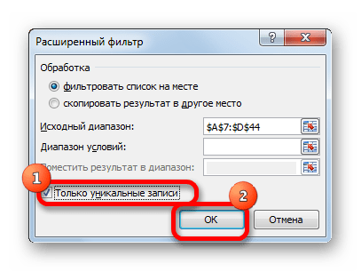
- Ставим флажок напротив «Скопировать результат в другое место» (1).
- Выбираем диапазон таблицы Excel, в который нужно поместить перечень уникальных строк (2).
- Устанавливаем галку напротив «Только уникальные записи» (3).
Должно выглядеть так:

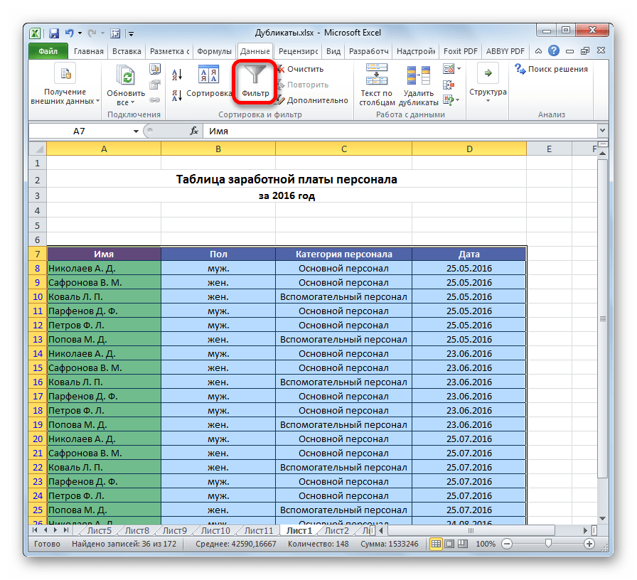
Шаг 4. Жмём «ОК» и видим, что у нас теперь 2 списка.

Второй короче первого, поскольку одна из Свет «отправилась восвояси». Строки с именем «Света» дублировались по всем параметрам.
Просто, не так ли? Правда, удаление дублей в Excel 2013 таким способом не позволяет отфильтровать строки, которые сходятся по одному или двум критериям – например, сохранить в перечне только девушек с уникальными именами. Останутся две «Лены», поскольку они разного роста. Более гибкий фильтр можно настроить, прибегнув к следующему методу.
Как убрать дубли в Excel через функцию «Удалить дубликаты»
Этот способ ещё проще. Действуем так:
Шаг 1. Переходим в раздел «Данные» в главном меню и кликаем на кнопку «Удалить дубликаты» (в блоке «Работа c данными»).

Шаг 2. Появится такое окно:

В этом окне нужно сначала поставить галку напротив «Мои данные содержат заголовки» (конечно, если заголовки у столбцов есть), следом выбрать параметры (тут внимание!), при единовременном совпадении которых строка будет удалена из перечня.
Приведу пример. Мы хотим оставить в таблице только один вариант женского пола (параметр «Пол») и ростом 159 см (параметр «Рост»). Значит, в окошке выделяем колонки «Пол» и «Рост». Жмём «ОК».

И вот что у нас получилось:

Из 159-сантиметровых девушек осталась только первая Света. Катя и вторая Света, имея аналогичный рост, оказались исключены из таблицы. Сама таблица сократилась до 8 строчек.
Поиск одинаковых значений в Excel
Выберем одну из ячеек в таблице. Рассмотрим, как в Экселе найти повторяющиеся значения, равные содержимому ячейки, и выделить их цветом.
На рисунке – списки писателей. Алгоритм действий следующий:
- Выбрать ячейку I3 с записью «С. А. Есенин».
- Поставить задачу – выделить цветом ячейки с такими же записями.
- Выделить область поисков.
- Нажать вкладку «Главная».
- Далее группа «Стили».
- Затем «Условное форматирование»;
- Нажать команду «Равно».

- Появится диалоговое окно:

- В левом поле указать ячейку с I2, в которой записано «С. А. Есенин».
- В правом поле можно выбрать цвет шрифта.
- Нажать «ОК».
В таблицах отмечены цветом ячейки, значение которых равно заданному.

Несложно понять, как в Экселе найти одинаковые значения в столбце. Просто выделить перед поиском нужную область – конкретный столбец.
Ищем в таблицах Excel все повторяющиеся значения
Отметим все неуникальные записи в выделенной области. Для этого нужно:
- Зайти в группу «Стили».
- Далее «Условное форматирование».
- Теперь в выпадающем меню выбрать «Правила выделения ячеек».
- Затем «Повторяющиеся значения».

- Появится диалоговое окно:

- Нажать «ОК».
Программа ищет повторения во всех столбцах.

Если в таблице много неуникальных записей, то информативность такого поиска сомнительна.
Удаление одинаковых значений из таблицы Excel
Способ удаления неуникальных записей:
- Зайти во вкладку «Данные».
- Выделить столбец, в котором следует искать дублирующиеся строки.
- Опция «Удалить дубликаты».

В результате получаем список, в котором каждое имя фигурирует только один раз.

Список с уникальными значениями:

Расширенный фильтр: оставляем только уникальные записи
Расширенный фильтр – это инструмент для получения упорядоченного списка с уникальными записями.
- Выбрать вкладку «Данные».
- Перейти в раздел «Сортировка и фильтр».
- Нажать команду «Дополнительно»:

- В появившемся диалоговом окне ставим флажок «Только уникальные записи».
- Нажать «OK» – уникальный список готов.
Поиск дублирующихся значений с помощью сводных таблиц
Составим список уникальных строк, не теряя данные из других столбцов и не меняя исходную таблицу. Для этого используем инструмент Сводная таблица:
Вкладка «Вставка».
Пункт «Сводная таблица».

В диалоговом окне выбрать размещение сводной таблицы на новом листе.

В открывшемся окне отмечаем столбец, в котором содержатся интересующие нас значений.

Заключение
Excel предлагает несколько инструментов для нахождения и удаления строк или ячеек с одинаковыми данными. Каждый из описанных методов специфичен и имеет свои ограничения. К универсальным варианту мы, пожалуй, отнесем использование “умной таблицы” и функции “Удалить дубликаты”. В целом, для выполнения поставленной задачи необходимо руководствоваться как особенностями структуры таблицы, так и преследуемыми целями и видением конечного результата.
Источники
- https://exceltable.com/sozdat-tablicu/udalenie-dublikatov-v-excel
- https://naprimerax.org/posts/67/udalit-dublikaty-v-excel
- https://www.nibbl.ru/office/excel-kak-udalit-dublikaty-no-ostavit-unikalnye-znacheniya.html
- https://office-guru.ru/excel/udalenie-dublikatov-strok-v-excel-139.html
- https://excelhack.ru/kak-udalit-dublikaty-v-excel/
- https://MicroExcel.ru/udalenie-dublikatov/
- https://kovalev-copyright.ru/metodologicheskie-osnovy-dlya-kopirajterov/kak-udalit-povtoryayushhiesya-stroki-v-excel.html
- https://FreeSoft.ru/blog/kak-v-excel-nayti-povtoryayushchiesya-i-odinakovye-znacheniya
Содержание
- Поиск и удаление
- Способ 1: простое удаление повторяющихся строк
- Способ 2: удаление дубликатов в «умной таблице»
- Способ 3: применение сортировки
- Способ 4: условное форматирование
- Способ 5: применение формулы
- Вопросы и ответы

При работе с таблицей или базой данных с большим количеством информации возможна ситуация, когда некоторые строки повторяются. Это ещё больше увеличивает массив данных. К тому же, при наличии дубликатов возможен некорректный подсчет результатов в формулах. Давайте разберемся, как в программе Microsoft Excel отыскать и удалить повторяющиеся строки.
Поиск и удаление
Найти и удалить значения таблицы, которые дублируются, возможно разными способами. В каждом из этих вариантов поиск и ликвидация дубликатов – это звенья одного процесса.
Способ 1: простое удаление повторяющихся строк
Проще всего удалить дубликаты – это воспользоваться специальной кнопкой на ленте, предназначенной для этих целей.
- Выделяем весь табличный диапазон. Переходим во вкладку «Данные». Жмем на кнопку «Удалить дубликаты». Она располагается на ленте в блоке инструментов «Работа с данными».
- Открывается окно удаление дубликатов. Если у вас таблица с шапкой (а в подавляющем большинстве всегда так и есть), то около параметра «Мои данные содержат заголовки» должна стоять галочка. В основном поле окна расположен список столбцов, по которым будет проводиться проверка. Строка будет считаться дублем только в случае, если данные всех столбцов, выделенных галочкой, совпадут. То есть, если вы снимете галочку с названия какого-то столбца, то тем самым расширяете вероятность признания записи повторной. После того, как все требуемые настройки произведены, жмем на кнопку «OK».
- Excel выполняет процедуру поиска и удаления дубликатов. После её завершения появляется информационное окно, в котором сообщается, сколько повторных значений было удалено и количество оставшихся уникальных записей. Чтобы закрыть данное окно, жмем кнопку «OK».

Способ 2: удаление дубликатов в «умной таблице»
Дубликаты можно удалить из диапазона ячеек, создав умную таблицу.
- Выделяем весь табличный диапазон.
- Находясь во вкладке «Главная» жмем на кнопку «Форматировать как таблицу», расположенную на ленте в блоке инструментов «Стили». В появившемся списке выбираем любой понравившийся стиль.
- Затем открывается небольшое окошко, в котором нужно подтвердить выбранный диапазон для формирования «умной таблицы». Если вы выделили все правильно, то можно подтверждать, если допустили ошибку, то в этом окне следует исправить. Важно также обратить внимание на то, чтобы около параметра «Таблица с заголовками» стояла галочка. Если её нет, то следует поставить. После того, как все настройки завершены, жмите на кнопку «OK». «Умная таблица» создана.
- Но создание «умной таблицы» — это только один шаг для решения нашей главной задачи – удаления дубликатов. Кликаем по любой ячейке табличного диапазона. При этом появляется дополнительная группа вкладок «Работа с таблицами». Находясь во вкладке «Конструктор» кликаем по кнопке «Удалить дубликаты», которая расположена на ленте в блоке инструментов «Сервис».
- После этого, открывается окно удаления дубликатов, работа с которым была подробно расписана при описании первого способа. Все дальнейшие действия производятся в точно таком же порядке.

Этот способ является наиболее универсальным и функциональным из всех описанных в данной статье.
Урок: Как сделать таблицу в Excel
Способ 3: применение сортировки
Данный способ является не совсем удалением дубликатов, так как сортировка только скрывает повторные записи в таблице.

- Выделяем таблицу. Переходим во вкладку «Данные». Жмем на кнопку «Фильтр», расположенную в блоке настроек «Сортировка и фильтр».
- Фильтр включен, о чем говорят появившиеся пиктограммы в виде перевернутых треугольников в названиях столбцов. Теперь нам нужно его настроить. Кликаем по кнопке «Дополнительно», расположенной рядом все в той же группе инструментов «Сортировка и фильтр».
- Открывается окно расширенного фильтра. Устанавливаем в нем галочку напротив параметра «Только уникальные записи». Все остальные настройки оставляем по умолчанию. После этого кликаем по кнопке «OK».
После этого, повторяющиеся записи будут скрыты. Но их показ можно в любой момент включить повторным нажатием на кнопку «Фильтр».
Урок: Расширенный фильтр в Excel
Способ 4: условное форматирование
Найти повторяющиеся ячейки можно также при помощи условного форматирования таблицы. Правда, удалять их придется другим инструментом.
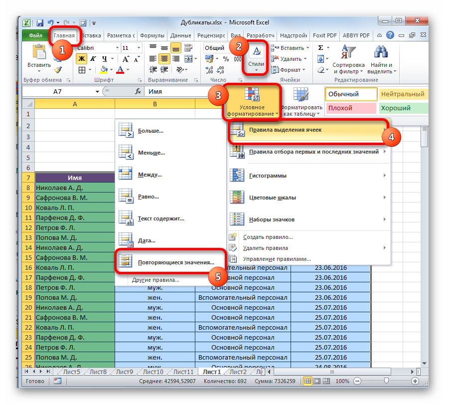
- Выделяем область таблицы. Находясь во вкладке «Главная», жмем на кнопку «Условное форматирование», расположенную в блоке настроек «Стили». В появившемся меню последовательно переходим по пунктам «Правила выделения» и «Повторяющиеся значения…».
- Открывается окно настройки форматирования. Первый параметр в нём оставляем без изменения – «Повторяющиеся». А вот в параметре выделения можно, как оставить настройки по умолчанию, так и выбрать любой подходящий для вас цвет, после этого жмем на кнопку «OK».

После этого произойдет выделение ячеек с повторяющимися значениями. Эти ячейки вы потом при желании сможете удалить вручную стандартным способом.
Внимание! Поиск дублей с применением условного форматирования производится не по строке в целом, а по каждой ячейке в частности, поэтому не для всех случаев он является подходящим.
Урок: Условное форматирование в Excel
Способ 5: применение формулы
Кроме того, найти дубликаты можно применив формулу с использованием сразу нескольких функций. С её помощью можно производить поиск дубликатов по конкретному столбцу. Общий вид данной формулы будет выглядеть следующим образом:
=ЕСЛИОШИБКА(ИНДЕКС(адрес_столбца;ПОИСКПОЗ(0;СЧЁТЕСЛИ(адрес_шапки_столбца_дубликатов: адрес_шапки_столбца_дубликатов (абсолютный); адрес_столбца;)+ЕСЛИ(СЧЁТЕСЛИ(адрес_столбца;; адрес_столбца;)>1;0;1);0));"")
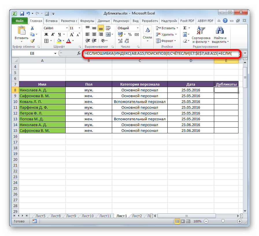
- Создаем отдельный столбец, куда будут выводиться дубликаты.
- Вводим формулу по указанному выше шаблону в первую свободную ячейку нового столбца. В нашем конкретном случае формула будет иметь следующий вид:
=ЕСЛИОШИБКА(ИНДЕКС(A8:A15;ПОИСКПОЗ(0;СЧЁТЕСЛИ(E7:$E$7;A8:A15)+ЕСЛИ(СЧЁТЕСЛИ(A8:A15;A8:A15)>1;0;1);0));"") - Выделяем весь столбец для дубликатов, кроме шапки. Устанавливаем курсор в конец строки формул. Нажимаем на клавиатуре кнопку F2. Затем набираем комбинацию клавиш Ctrl+Shift+Enter. Это обусловлено особенностями применения формул к массивам.
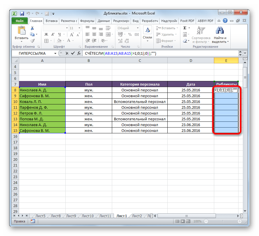
После этих действий в столбце «Дубликаты» отобразятся повторяющиеся значения.
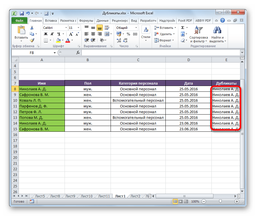
Но, данный способ все-таки слишком сложен для большинства пользователей. К тому же, он предполагает только поиск дублей, но не их удаление. Поэтому рекомендуется применять более простые и функциональные решения, описанные ранее.
Как видим, в Экселе есть множество инструментов предназначенных для поиска и удаления дублей. У каждого из них есть свои особенности. Например, условное форматирование предполагает поиск дублей только по каждой ячейке в отдельности. К тому же, не все инструменты могут не только искать, но и удалять повторяющиеся значения. Наиболее универсальный вариант – это создание «умной таблицы». При использовании данного способа можно максимально точно и удобно настроить поиск дубликатов. К тому же, их удаление происходит моментально.
Еще статьи по данной теме:
Помогла ли Вам статья?
This example teaches you how to remove duplicates in Excel.
1. Click any single cell inside the data set.
2. On the Data tab, in the Data Tools group, click Remove Duplicates.

The following dialog box appears.
3. Leave all check boxes checked and click OK.

Result. Excel removes all identical rows (blue) except for the first identical row found (yellow).


To remove rows with the same values in certain columns, execute the following steps.
4. For example, remove rows with the same Last Name and Country.
5. Check Last Name and Country and click OK.

Result. Excel removes all rows with the same Last Name and Country (blue) except for the first instances found (yellow).


Let’s take a look at one more cool Excel feature that removes duplicates. You can use the Advanced Filter to extract unique rows (or unique values in a column).
6. On the Data tab, in the Sort & Filter group, click Advanced.

The Advanced Filter dialog box appears.
7. Click Copy to another location.
8. Click in the List range box and select the range A1:A17 (see images below).
9. Click in the Copy to box and select cell F1 (see images below).
10. Check Unique records only.

11. Click OK.
Result. Excel removes all duplicate last names and sends the result to column F.

Note: at step 8, instead of selecting the range A1:A17, select the range A1:D17 to extract unique rows.
12. Finally, you can use conditional formatting in Excel to highlight duplicate values.

13. Or use conditional formatting in Excel to highlight duplicate rows.

Tip: visit our page about finding duplicates to learn more about these tricks.
How to Remove Duplicates in Excel (and Find Them)
In an Excel spreadsheet, you’d often have to collate data from multiple sources. Sometimes from external sources (like webpages) too 🖨
And this might result in duplicates in your Excel sheet. So how can you remove them? By scanning your worksheet for dupes manually?
Nah! That’s not going to work if you have a large dataset. Let’s think of a smarter solution 🧠
To find and remove duplicate values in Excel, you can use the Remove Duplicate tool of Excel (and some other easy ways too). To learn how, dive straight into the guide below.
Practice along with the guide by downloading our sample workbook here 📩
How to remove duplicates in excel
We will look into multiple methods of removing duplicates in Excel. Which one’s the best? I leave that to you 😅
So, here’s the list of names that have many instances of duplication.

We need to remove the duplicate values from this list.
Here are different methods that can help you do this✂
Advanced Filter
To remove duplicates values from your data using the advanced filters:
- Select the data that needs to be filtered.

- Go to the Data Tab > Advanced Filters.

This opens up the Advanced Filter dialog box as follows 👀

The list range is already selected (that’s because we selected the data to be filtered before launching the advanced filter) 👌
Pro Tip!
Under the box Action:

- Select Filter the list, in place if you want the original dataset to be de-duped.
- Select copy to another location if you don’t want to disturb the original data. This way Excel will ask you for a location (a cell range basically) where you want to create a copy of the source data. Duplicates will then be deleted from this copied set of data and your original data will remain the same.
- Check the option for Unique Records only. This tells Excel to delete any dupes from the dataset.

- Click Okay.
Here comes the data which no longer has duplicates 🤩

Note that we had selected the option to Filter in place so our original dataset has changed.
Remove Duplicates
Do you know Excel has an in-built feature for removing duplicates? We will explore that now 🔎
So with the same list of names, here we go:
- Select the column header for the column that contains the duplicate values (List of Names in our example).

- Go to the Data Tab > Remove Duplicates.

- Select the column from where the duplicates are to be removed. Note that it is already selected in our case.
- Check the box for “My data has headers” as highlighted below.

- Click Okay.
Excel brings you a dialog box that tells how many duplicate values have been found and removed. And how many unique values are retained. This way you can remove duplicates from each column of your dataset 🚀

Here is the deduped list. Excel has found and removed all instances of duplication 💪

UNIQUE function
Another way how you can extract unique (or other than duplicate values) from a dataset is by using the UNIQUE function.
The UNIQUE function extracts a list of unique values from a given set of values 📝
Must know that the UNIQUE function is a dynamic array function. It returns an array of unique values 📌
And as it is a dynamic array function, it is only available in the dynamic versions of Excel. Starting from Excel 2021 to Microsoft 365 only. The older (non-dynamic versions) of Excel do not support dynamic array functions.
So to extract a list of unique names from our dataset:
- Begin writing the UNIQUE function as follows ✍
= UNIQUE

- Specify the range that needs to be filtered.
= UNIQUE (A2:A8)

We want to remove dupes from the list of names i.e. Cell A2 to Cell A8. So we are creating a reference to these cells.
- Hit Enter, and there are your filtered values.

Pro Tip!
Instead of an array of unique values, did the UNIQUE function return the #SPILL error 🥴
That’s because your spill range is not empty (some cells might already have values). The spill range is the cell range (to the bottom or right of the active cell) where the UNIQUE function will populate the array of unique values.
How to find duplicates in excel
You’d enjoy the process of finding duplicates in Excel. Make sure you’re there with us till the end of it 🚴♀️
Continuing with the same list of names from our previous example.

This time we only need to find out the duplicate values from this list, so here we go.
- Select the data (from where you want to find the duplicates).

- Go to the Home Tab > Conditional Formatting.

- From the drop-down menu that appears, select Highlight Cell Rules > Duplicate values 🎨

This way the conditional formatting tool of Excel will highlight duplicates from the selected dataset.
Like in the image below.

We have all the duplicate data highlighted from our dataset above.
However, all the values are still mixed. Do you want to separate the duplicate values?
Do it through the steps below 👇
- Select the header for the subject column (List of Names in our example).
- Go to the Data tab > Filter.

Once the filters are applied, you’d see the filter icon (drop-down menu icon) inside the selected column header.
- Click on that drop-down menu icon 🔽
- From the context menu that opens up, select Sort by Color > Red.

And we have the highlighted values (duplicate values) filtered only.

You now may choose to cut/paste them, delete them or treat them in any way you like 🙈
That’s it – Now what?
The above article is a complete guide on how to find and remove duplicates in Excel. Like reading it?
If you did, you’d be amazed to know how versatile Microsoft Excel is. And the best part of Excel is that it has a huge (and that’s an emphasized huge) library of functions 📚
Each function of Excel is super smart and useful when used the right way. To master Excel functions, you must have a good grip on some core functions of Excel.
These include the VLOOKUP, SUMIF, and IF functions. To learn them, enroll in my 30-minute free email course now. It covers these (and many more) Excel functions, features, and tools.
Frequently asked questions
To delete duplicates from any dataset in Excel.
- Select the column header for the column that contains the duplicate values.
- Go to the Data Tab > Remove Duplicates.
- Under the Remove Duplicate dialog box, select the subject column.
- Check the box for “My data has headers” if the column has any.
- Click “Okay”.
To quickly delete duplicates, use the in-built tool for duplicate removal in Excel as below:
- Select the column header for the column that contains the duplicate values.
- Go to the Data Tab > Remove Duplicates.
- Under the Remove Duplicate dialog box, select the subject column.
Check the box for “My data has headers” if the column has any and click “OK”.
Kasper Langmann2023-01-21T18:45:48+00:00
Page load link