Excel and or nothing - Word и Excel - помощь в работе с программами

The IF function allows you to make a logical comparison between a value and what you expect by testing for a condition and returning a result if that condition is True or False.

=IF(Something is True, then do something, otherwise do something else)

But what if you need to test multiple conditions, where let’s say all conditions need to be True or False (AND), or only one condition needs to be True or False (OR), or if you want to check if a condition does NOT meet your criteria? All 3 functions can be used on their own, but it’s much more common to see them paired with IF functions.

Use the IF function along with AND, OR and NOT to perform multiple evaluations if conditions are True or False.

Syntax

IF(AND()) — IF(AND(logical1, [logical2], …), value_if_true, [value_if_false]))
IF(OR()) — IF(OR(logical1, [logical2], …), value_if_true, [value_if_false]))
IF(NOT()) — IF(NOT(logical1), value_if_true, [value_if_false]))


Argument name	Description
logical_test (required)	The condition you want to test.
value_if_true (required)	The value that you want returned if the result of logical_test is TRUE.

value_if_false (optional)	The value that you want returned if the result of logical_test is FALSE.

Here are overviews of how to structure AND, OR and NOT functions individually. When you combine each one of them with an IF statement, they read like this:

AND – =IF(AND(Something is True, Something else is True), Value if True, Value if False)
OR – =IF(OR(Something is True, Something else is True), Value if True, Value if False)
NOT – =IF(NOT(Something is True), Value if True, Value if False)

Examples

Following are examples of some common nested IF(AND()), IF(OR()) and IF(NOT()) statements. The AND and OR functions can support up to 255 individual conditions, but it’s not good practice to use more than a few because complex, nested formulas can get very difficult to build, test and maintain. The NOT function only takes one condition.

Here are the formulas spelled out according to their logic:

Formula	Description
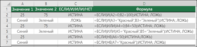
=IF(AND(A2>0,B2<100),TRUE, FALSE)	IF A2 (25) is greater than 0, AND B2 (75) is less than 100, then return TRUE, otherwise return FALSE. In this case both conditions are true, so TRUE is returned.
=IF(AND(A3=»Red»,B3=»Green»),TRUE,FALSE)	If A3 (“Blue”) = “Red”, AND B3 (“Green”) equals “Green” then return TRUE, otherwise return FALSE. In this case only the first condition is true, so FALSE is returned.
=IF(OR(A4>0,B4<50),TRUE, FALSE)	IF A4 (25) is greater than 0, OR B4 (75) is less than 50, then return TRUE, otherwise return FALSE. In this case, only the first condition is TRUE, but since OR only requires one argument to be true the formula returns TRUE.
=IF(OR(A5=»Red»,B5=»Green»),TRUE,FALSE)	IF A5 (“Blue”) equals “Red”, OR B5 (“Green”) equals “Green” then return TRUE, otherwise return FALSE. In this case, the second argument is True, so the formula returns TRUE.
=IF(NOT(A6>50),TRUE,FALSE)	IF A6 (25) is NOT greater than 50, then return TRUE, otherwise return FALSE. In this case 25 is not greater than 50, so the formula returns TRUE.
=IF(NOT(A7=»Red»),TRUE,FALSE)	IF A7 (“Blue”) is NOT equal to “Red”, then return TRUE, otherwise return FALSE.

Note that all of the examples have a closing parenthesis after their respective conditions are entered. The remaining True/False arguments are then left as part of the outer IF statement. You can also substitute Text or Numeric values for the TRUE/FALSE values to be returned in the examples.

Here are some examples of using AND, OR and NOT to evaluate dates.

Here are the formulas spelled out according to their logic:

Formula	Description
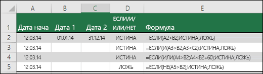
=IF(A2>B2,TRUE,FALSE)	IF A2 is greater than B2, return TRUE, otherwise return FALSE. 03/12/14 is greater than 01/01/14, so the formula returns TRUE.
=IF(AND(A3>B2,A3<C2),TRUE,FALSE)	IF A3 is greater than B2 AND A3 is less than C2, return TRUE, otherwise return FALSE. In this case both arguments are true, so the formula returns TRUE.
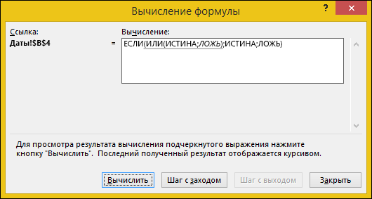
=IF(OR(A4>B2,A4<B2+60),TRUE,FALSE)	IF A4 is greater than B2 OR A4 is less than B2 + 60, return TRUE, otherwise return FALSE. In this case the first argument is true, but the second is false. Since OR only needs one of the arguments to be true, the formula returns TRUE. If you use the Evaluate Formula Wizard from the Formula tab you’ll see how Excel evaluates the formula.
=IF(NOT(A5>B2),TRUE,FALSE)	IF A5 is not greater than B2, then return TRUE, otherwise return FALSE. In this case, A5 is greater than B2, so the formula returns FALSE.

Using AND, OR and NOT with Conditional Formatting

You can also use AND, OR and NOT to set Conditional Formatting criteria with the formula option. When you do this you can omit the IF function and use AND, OR and NOT on their own.

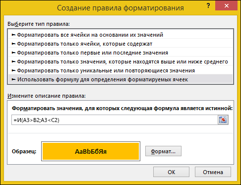
From the Home tab, click Conditional Formatting > New Rule. Next, select the “Use a formula to determine which cells to format” option, enter your formula and apply the format of your choice.

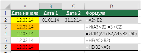
Using the earlier Dates example, here is what the formulas would be.

Formula	Description
=A2>B2	If A2 is greater than B2, format the cell, otherwise do nothing.
=AND(A3>B2,A3<C2)	If A3 is greater than B2 AND A3 is less than C2, format the cell, otherwise do nothing.
=OR(A4>B2,A4<B2+60)	If A4 is greater than B2 OR A4 is less than B2 plus 60 (days), then format the cell, otherwise do nothing.
=NOT(A5>B2)	If A5 is NOT greater than B2, format the cell, otherwise do nothing. In this case A5 is greater than B2, so the result will return FALSE. If you were to change the formula to =NOT(B2>A5) it would return TRUE and the cell would be formatted.

Note: A common error is to enter your formula into Conditional Formatting without the equals sign (=). If you do this you’ll see that the Conditional Formatting dialog will add the equals sign and quotes to the formula — =»OR(A4>B2,A4<B2+60)», so you’ll need to remove the quotes before the formula will respond properly.

Need more help?

Use AND and OR to test a combination of conditions

When you need to find data that meets more than one condition, such as units sold between April and January, or units sold by Nancy, you can use the AND and OR functions together. Here’s an example:

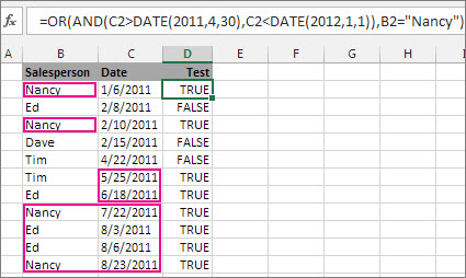
This formula nests the AND function inside the OR function to search for units sold between April 1, 2011 and January 1, 2012, or any units sold by Nancy. You can see it returns True for units sold by Nancy, and also for units sold by Tim and Ed during the dates specified in the formula.

Here’s the formula in a form you can copy and paste. If you want to play with it in a sample workbook, see the end of this article.

Use AND and OR with IF

You can also use AND and OR with the IF function.

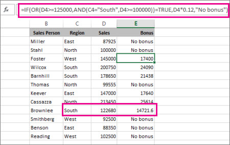
In this example, people don’t earn bonuses until they sell at least $125,000 worth of goods, unless they work in the southern region where the market is smaller. In that case, they qualify for a bonus after $100,000 in sales.

Let’s look a bit deeper. The IF function requires three pieces of data (arguments) to run properly. The first is a logical test, the second is the value you want to see if the test returns True, and the third is the value you want to see if the test returns False. In this example, the OR function and everything nested in it provides the logical test. You can read it as: Look for values greater than or equal to 125,000, unless the value in column C is «South», then look for a value greater than 100,000, and every time both conditions are true, multiply the value by 0.12, the commission amount. Otherwise, display the words «No bonus.»

Sample data

If you want to work with the examples in this article, copy the following table into cell A1 in your own spreadsheet. Be sure to select the whole table, including the heading row.

Источник

Использование ЕСЛИ с функциями И, ИЛИ и НЕ

Функция ЕСЛИ позволяет выполнять логические сравнения значений и ожидаемых результатов. Она проверяет условие и в зависимости от его истинности возвращает результат.

=ЕСЛИ(это истинно, то сделать это, в противном случае сделать что-то еще)

Но что делать, если необходимо проверить несколько условий, где, допустим, все условия должны иметь значение ИСТИНА или ЛОЖЬ ( И), только одно условие должно иметь такое значение ( ИЛИ) или вы хотите убедиться, что данные НЕ соответствуют условию? Эти три функции можно использовать самостоятельно, но они намного чаще встречаются в сочетании с функцией ЕСЛИ.

Используйте функцию ЕСЛИ вместе с функциями И, ИЛИ и НЕ, чтобы оценивать несколько условий.

ЕСЛИ(И()): ЕСЛИ(И(лог_выражение1; [лог_выражение2]; …), значение_если_истина; [значение_если_ложь]))

ЕСЛИ(ИЛИ()): ЕСЛИ(ИЛИ(лог_выражение1; [лог_выражение2]; …), значение_если_истина; [значение_если_ложь]))

ЕСЛИ(НЕ()): ЕСЛИ(НЕ(лог_выражение1), значение_если_истина; [значение_если_ложь]))

Условие, которое нужно проверить.

Значение, которое должно возвращаться, если лог_выражение имеет значение ИСТИНА.

Значение, которое должно возвращаться, если лог_выражение имеет значение ЛОЖЬ.

Общие сведения об использовании этих функций по отдельности см. в следующих статьях: И, ИЛИ, НЕ. При сочетании с оператором ЕСЛИ они расшифровываются следующим образом:

И: =ЕСЛИ(И(условие; другое условие); значение, если ИСТИНА; значение, если ЛОЖЬ)

ИЛИ: =ЕСЛИ(ИЛИ(условие; другое условие); значение, если ИСТИНА; значение, если ЛОЖЬ)

НЕ: =ЕСЛИ(НЕ(условие); значение, если ИСТИНА; значение, если ЛОЖЬ)

Примеры

Ниже приведены примеры распространенных случаев использования вложенных операторов ЕСЛИ(И()), ЕСЛИ(ИЛИ()) и ЕСЛИ(НЕ()). Функции И и ИЛИ поддерживают до 255 отдельных условий, но рекомендуется использовать только несколько условий, так как формулы с большой степенью вложенности сложно создавать, тестировать и изменять. У функции НЕ может быть только одно условие.

Ниже приведены формулы с расшифровкой их логики.

=ЕСЛИ(И(A2>0;B2 0;B4 50);ИСТИНА;ЛОЖЬ)

Если A6 (25) НЕ больше 50, возвращается значение ИСТИНА, в противном случае возвращается значение ЛОЖЬ. В этом случае значение не больше чем 50, поэтому формула возвращает значение ИСТИНА.

Если значение A7 («синий») НЕ равно «красный», возвращается значение ИСТИНА, в противном случае возвращается значение ЛОЖЬ.

Обратите внимание, что во всех примерах есть закрывающая скобка после условий. Аргументы ИСТИНА и ЛОЖЬ относятся ко внешнему оператору ЕСЛИ. Кроме того, вы можете использовать текстовые или числовые значения вместо значений ИСТИНА и ЛОЖЬ, которые возвращаются в примерах.

Вот несколько примеров использования операторов И, ИЛИ и НЕ для оценки дат.

Ниже приведены формулы с расшифровкой их логики.

Если A2 больше B2, возвращается значение ИСТИНА, в противном случае возвращается значение ЛОЖЬ. В этом случае 12.03.14 больше чем 01.01.14, поэтому формула возвращает значение ИСТИНА.

=ЕСЛИ(И(A3>B2;A3 B2;A4 B2);ИСТИНА;ЛОЖЬ)

Если A5 не больше B2, возвращается значение ИСТИНА, в противном случае возвращается значение ЛОЖЬ. В этом случае A5 больше B2, поэтому формула возвращает значение ЛОЖЬ.

Использование операторов И, ИЛИ и НЕ с условным форматированием

Вы также можете использовать операторы И, ИЛИ и НЕ в формулах условного форматирования. При этом вы можете опустить функцию ЕСЛИ.

На вкладке Главная выберите Условное форматирование > Создать правило. Затем выберите параметр Использовать формулу для определения форматируемых ячеек, введите формулу и примените формат.

«Изменить правило» с параметром «Формула»» loading=»lazy»>

Вот как будут выглядеть формулы для примеров с датами:

Если A2 больше B2, отформатировать ячейку, в противном случае не выполнять никаких действий.

=И(A3>B2;A3 B2;A4 B2)

Если A5 НЕ больше B2, отформатировать ячейку, в противном случае не выполнять никаких действий. В этом случае A5 больше B2, поэтому формула возвращает значение ЛОЖЬ. Если изменить формулу на =НЕ(B2>A5), она вернет значение ИСТИНА, а ячейка будет отформатирована.

Примечание: Распространенной ошибкой является ввод формулы в условное форматирование без знака равенства (=). В этом случае вы увидите, что диалоговое окно Условное форматирование добавит знак равенства и кавычки в формулу — =»OR(A4>B2,A4

Дополнительные сведения

См. также

Вы всегда можете задать вопрос специалисту Excel Tech Community или попросить помощи в сообществе Answers community.

Источник

Using IF with AND, OR and NOT functions

The IF function allows you to make a logical comparison between a value and what you expect by testing for a condition and returning a result if that condition is True or False.

=IF(Something is True, then do something, otherwise do something else)

But what if you need to test multiple conditions, where let’s say all conditions need to be True or False ( AND), or only one condition needs to be True or False ( OR), or if you want to check if a condition does NOT meet your criteria? All 3 functions can be used on their own, but it’s much more common to see them paired with IF functions.

Use the IF function along with AND, OR and NOT to perform multiple evaluations if conditions are True or False.

IF(AND()) — IF(AND(logical1, [logical2], . ), value_if_true, [value_if_false]))

IF(OR()) — IF(OR(logical1, [logical2], . ), value_if_true, [value_if_false]))

IF(NOT()) — IF(NOT(logical1), value_if_true, [value_if_false]))

The condition you want to test.

The value that you want returned if the result of logical_test is TRUE.

The value that you want returned if the result of logical_test is FALSE.

Here are overviews of how to structure AND, OR and NOT functions individually. When you combine each one of them with an IF statement, they read like this:

AND – =IF(AND(Something is True, Something else is True), Value if True, Value if False)

OR – =IF(OR(Something is True, Something else is True), Value if True, Value if False)

NOT – =IF(NOT(Something is True), Value if True, Value if False)

Examples

Here are the formulas spelled out according to their logic:

=IF(AND(A2>0,B2 0,B4 50),TRUE,FALSE)

IF A6 (25) is NOT greater than 50, then return TRUE, otherwise return FALSE. In this case 25 is not greater than 50, so the formula returns TRUE.

IF A7 (“Blue”) is NOT equal to “Red”, then return TRUE, otherwise return FALSE.

Here are some examples of using AND, OR and NOT to evaluate dates.

Here are the formulas spelled out according to their logic:

IF A2 is greater than B2, return TRUE, otherwise return FALSE. 03/12/14 is greater than 01/01/14, so the formula returns TRUE.

=IF(AND(A3>B2,A3 B2,A4 B2),TRUE,FALSE)

IF A5 is not greater than B2, then return TRUE, otherwise return FALSE. In this case, A5 is greater than B2, so the formula returns FALSE.

Using AND, OR and NOT with Conditional Formatting

You can also use AND, OR and NOT to set Conditional Formatting criteria with the formula option. When you do this you can omit the IF function and use AND, OR and NOT on their own.

From the Home tab, click Conditional Formatting > New Rule. Next, select the “ Use a formula to determine which cells to format” option, enter your formula and apply the format of your choice.

Edit Rule dialog showing the Formula method» loading=»lazy»>

Using the earlier Dates example, here is what the formulas would be.

If A2 is greater than B2, format the cell, otherwise do nothing.

=AND(A3>B2,A3 B2,A4 B2)

If A5 is NOT greater than B2, format the cell, otherwise do nothing. In this case A5 is greater than B2, so the result will return FALSE. If you were to change the formula to =NOT(B2>A5) it would return TRUE and the cell would be formatted.

Note: A common error is to enter your formula into Conditional Formatting without the equals sign (=). If you do this you’ll see that the Conditional Formatting dialog will add the equals sign and quotes to the formula — =»OR(A4>B2,A4

Need more help?

Using IF with AND, OR and NOT functions

The IF function allows you to make a logical comparison between a value and what you expect by testing for a condition and returning a result if that condition is True or False.

=IF(Something is True, then do something, otherwise do something else)

Use the IF function along with AND, OR and NOT to perform multiple evaluations if conditions are True or False.

IF(AND()) — IF(AND(logical1, [logical2], . ), value_if_true, [value_if_false]))

IF(OR()) — IF(OR(logical1, [logical2], . ), value_if_true, [value_if_false]))

IF(NOT()) — IF(NOT(logical1), value_if_true, [value_if_false]))

The condition you want to test.

The value that you want returned if the result of logical_test is TRUE.

The value that you want returned if the result of logical_test is FALSE.

Here are overviews of how to structure AND, OR and NOT functions individually. When you combine each one of them with an IF statement, they read like this:

AND – =IF(AND(Something is True, Something else is True), Value if True, Value if False)

OR – =IF(OR(Something is True, Something else is True), Value if True, Value if False)

NOT – =IF(NOT(Something is True), Value if True, Value if False)

Examples

Here are the formulas spelled out according to their logic:

=IF(AND(A2>0,B2 0,B4 50),TRUE,FALSE)

IF A6 (25) is NOT greater than 50, then return TRUE, otherwise return FALSE. In this case 25 is not greater than 50, so the formula returns TRUE.

IF A7 (“Blue”) is NOT equal to “Red”, then return TRUE, otherwise return FALSE.

Here are some examples of using AND, OR and NOT to evaluate dates.

Here are the formulas spelled out according to their logic:

IF A2 is greater than B2, return TRUE, otherwise return FALSE. 03/12/14 is greater than 01/01/14, so the formula returns TRUE.

=IF(AND(A3>B2,A3 B2,A4 B2),TRUE,FALSE)

IF A5 is not greater than B2, then return TRUE, otherwise return FALSE. In this case, A5 is greater than B2, so the formula returns FALSE.

Using AND, OR and NOT with Conditional Formatting

You can also use AND, OR and NOT to set Conditional Formatting criteria with the formula option. When you do this you can omit the IF function and use AND, OR and NOT on their own.

From the Home tab, click Conditional Formatting > New Rule. Next, select the “ Use a formula to determine which cells to format” option, enter your formula and apply the format of your choice.

Edit Rule dialog showing the Formula method» loading=»lazy»>

Using the earlier Dates example, here is what the formulas would be.

If A2 is greater than B2, format the cell, otherwise do nothing.

=AND(A3>B2,A3 B2,A4 B2)

Need more help?

Как использовать функцию IF

Функция IF — это основная логическая функция в Excel, и поэтому она должна быть понятна первой. Он появится много раз на протяжении всей этой статьи.

Давайте посмотрим на структуру функции IF, а затем посмотрим несколько примеров ее использования.

Функция IF принимает 3 бита информации:

  = IF (логический_тест, [value_if_true], [value_if_false])

логический_тест: это условие для функции для проверки.
value_if_true: действие, которое выполняется, если условие выполнено или является истинным.
value_if_false: действие, которое нужно выполнить, если условие не выполнено или имеет значение false.

Операторы сравнения для использования с логическими функциями

При выполнении логического теста со значениями ячеек вы должны быть знакомы с операторами сравнения. Вы можете увидеть их в таблице ниже.

Теперь давайте посмотрим на некоторые примеры в действии.

Пример функции IF 1: текстовые значения

В этом примере мы хотим проверить, равна ли ячейка определенной фразе. Функция IF не учитывает регистр, поэтому не учитывает прописные и строчные буквы.

Следующая формула используется в столбце C для отображения «Нет», если столбец B содержит текст «Завершено» и «Да», если он содержит что-либо еще.

  = ЕСЛИ (B2 = "Завершено", "Нет", "Да")

Хотя функция IF не чувствительна к регистру, текст должен точно соответствовать.

Пример функции IF 2: Числовые значения

Функция IF также отлично подходит для сравнения числовых значений.

В приведенной ниже формуле мы проверяем, содержит ли ячейка B2 число, большее или равное 75. Если это так, то мы отображаем слово «Pass», а если не слово «Fail».

  = ЕСЛИ (В2> = 75, "Проход", "Сбой")

Функция IF — это намного больше, чем просто отображение разного текста в результате теста. Мы также можем использовать его для запуска различных расчетов.

В этом примере мы хотим предоставить скидку 10%, если клиент тратит определенную сумму денег. Мы будем использовать £ 3000 в качестве примера.

  = ЕСЛИ (В2> = 3000, В2 * 90%, В2)

Часть формулы B2 * 90% позволяет вычесть 10% из значения в ячейке B2. Есть много способов сделать это.

Важно то, что вы можете использовать любую формулу в разделах value_if_true или value_if_false . И запускать различные формулы, зависящие от значений других ячеек, — очень мощный навык.

Пример функции IF 3: значения даты

В этом третьем примере мы используем функцию IF для отслеживания списка сроков исполнения. Мы хотим отобразить слово «Просрочено», если дата в столбце B уже в прошлом. Но если дата наступит в будущем, рассчитайте количество дней до даты исполнения.

Приведенная ниже формула используется в столбце C. Мы проверяем, меньше ли срок оплаты в ячейке B2, чем сегодняшний день (функция TODAY возвращает сегодняшнюю дату с часов компьютера).

  = ЕСЛИ (В2 <СЕГОДНЯ (), "Просроченные", В2-СЕГОДНЯ ())

Что такое вложенные формулы IF?

Возможно, вы слышали о термине «вложенные IF» раньше. Это означает, что мы можем написать функцию IF внутри другой функции IF. Мы можем захотеть сделать это, если нам нужно выполнить более двух действий.

Одна функция IF способна выполнять два действия ( value_if_true и value_if_false ). Но если мы вставим (или вложим) другую функцию IF в раздел value_if_false , то мы можем выполнить другое действие.

Возьмите этот пример, где мы хотим отобразить слово «Отлично», если значение в ячейке B2 больше или равно 90, отобразить «Хорошо», если значение больше или равно 75, и отобразить «Плохо», если что-либо еще ,

  = ЕСЛИ (В2> = 90, "Отлично", ЕСЛИ (В2> = 75, "Хорошо", "Плохо"))

Теперь мы расширили нашу формулу за пределы того, что может сделать только одна функция IF. И вы можете вложить больше функций IF, если это необходимо.

Обратите внимание на две закрывающие скобки в конце формулы — по одной для каждой функции IF.

Существуют альтернативные формулы, которые могут быть чище, чем этот вложенный подход IF. Одной из очень полезных альтернатив является функция SWITCH в Excel .

Логические функции AND и OR

Функции AND и OR используются, когда вы хотите выполнить более одного сравнения в своей формуле. Одна только функция IF может обрабатывать только одно условие или сравнение.

Возьмите пример, где мы дисконтируем значение на 10% в зависимости от суммы, которую тратит клиент, и сколько лет они были клиентом.

Сами функции AND и OR возвращают значение TRUE или FALSE.

Функция AND возвращает TRUE, только если выполняется каждое условие, а в противном случае возвращает FALSE. Функция OR возвращает TRUE, если выполняется одно или все условия, и возвращает FALSE, только если условия не выполняются.

Эти функции могут тестировать до 255 условий, поэтому они не ограничены только двумя условиями, как показано здесь.

Ниже приведена структура функций И и ИЛИ. Они написаны одинаково. Просто замените имя И на ИЛИ. Это просто их логика, которая отличается.

  = И (логический1, [логический2] ...)

Давайте посмотрим на пример того, как они оба оценивают два условия.

Пример функции AND

Функция AND используется ниже, чтобы проверить, потратил ли клиент не менее 3000 фунтов стерлингов и был ли он клиентом не менее трех лет.

  = И (В2> = 3000, С2> = 3)

Вы можете видеть, что он возвращает FALSE для Мэтта и Терри, потому что, хотя они оба соответствуют одному из критериев, они должны соответствовать обеим функциям AND.

Пример функции OR

Функция ИЛИ используется ниже, чтобы проверить, потратил ли клиент не менее 3000 фунтов стерлингов или был клиентом не менее трех лет.

  = ИЛИ (В2> = 3000, С2> = 3)

В этом примере формула возвращает TRUE для Matt и Terry. Только Джули и Джиллиан не выполняют оба условия и возвращают значение FALSE.

Использование AND и OR с функцией IF

Поскольку функции И и ИЛИ возвращают значение ИСТИНА или ЛОЖЬ, когда используются по отдельности, они редко используются сами по себе.

Вместо этого вы обычно будете использовать их с функцией IF или внутри функции Excel, такой как условное форматирование или проверка данных, чтобы выполнить какое-либо ретроспективное действие, если формула имеет значение TRUE.

В приведенной ниже формуле функция AND вложена в логический тест функции IF. Если функция AND возвращает TRUE, тогда скидка 10% от суммы в столбце B; в противном случае скидка не предоставляется, а значение в столбце B повторяется в столбце D.

  = ЕСЛИ (И (В2> = 3000, С2> = 3), В2 * 90%, В2)

Функция XOR

В дополнение к функции ИЛИ, есть также эксклюзивная функция ИЛИ. Это называется функцией XOR. Функция XOR была представлена в версии Excel 2013.

Эта функция может потребовать некоторых усилий, чтобы понять, поэтому практический пример показан.

Структура функции XOR такая же, как у функции OR.

  = XOR (логический1, [логический2] ...)

При оценке только двух условий функция XOR возвращает:

ИСТИНА, если любое условие оценивается как ИСТИНА.
FALSE, если оба условия TRUE или ни одно из условий TRUE.

Это отличается от функции ИЛИ, потому что она вернула бы ИСТИНА, если оба условия были ИСТИНА.

Эта функция становится немного более запутанной, когда добавляется больше условий. Затем функция XOR возвращает:

TRUE, если нечетное число условий возвращает TRUE.
ЛОЖЬ, если четное число условий приводит к ИСТИНА, или если все условия ЛОЖЬ.

Давайте посмотрим на простой пример функции XOR.

В этом примере продажи делятся на две половины года. Если продавец продает 3000 и более фунтов стерлингов в обеих половинах, ему назначается Золотой стандарт. Это достигается с помощью функции AND с IF, как ранее в этой статье.

Но если они продают 3000 фунтов или более в любой половине, мы хотим присвоить им Серебряный статус. Если они не продают 3000 и более фунтов стерлингов в обоих случаях, то ничего.

Функция XOR идеально подходит для этой логики. Приведенная ниже формула вводится в столбец E и показывает функцию XOR с IF для отображения «Да» или «Нет», только если выполняется любое из условий.

  = IF (XOR (В2> = 3000, С2> = 3000), "Да", "Нет")

Функция НЕ

Последняя логическая функция для обсуждения в этой статье — это функция NOT, и мы оставим самую простую последнюю. Хотя иногда поначалу бывает трудно увидеть использование этой функции в реальном мире.

Функция NOT меняет значение своего аргумента. Так что, если логическое значение ИСТИНА, тогда оно возвращает ЛОЖЬ. И если логическое значение ЛОЖЬ, оно вернет ИСТИНА.

Это будет легче объяснить на некоторых примерах.

Структура функции НЕ имеет вид;

  = НЕ (логическое)

НЕ Функциональный Пример 1

В этом примере представьте, что у нас есть головной офис в Лондоне, а затем много других региональных сайтов. Мы хотим отобразить слово «Да», если на сайте есть что-то, кроме Лондона, и «Нет», если это Лондон.

Функция NOT была вложена в логический тест функции IF ниже, чтобы сторнировать ИСТИННЫЙ результат.

  = ЕСЛИ (НЕ (B2 = "London"), "Да", "Нет")

Это также может быть достигнуто с помощью логического оператора NOT <>. Ниже приведен пример.

  = ЕСЛИ (В2 <> "Лондон", "Да", "Нет")

НЕ Функциональный Пример 2

Функция NOT полезна при работе с информационными функциями в Excel. Это группа функций в Excel, которые что-то проверяют и возвращают TRUE, если проверка прошла успешно, и FALSE, если это не так.

Например, функция ISTEXT проверит, содержит ли ячейка текст, и вернет TRUE, если она есть, и FALSE, если нет. Функция NOT полезна, потому что она может отменить результат этих функций.

В приведенном ниже примере мы хотим заплатить продавцу 5% от суммы, которую он продает. Но если они ничего не перепродали, в ячейке есть слово «Нет», и это приведет к ошибке в формуле.

Функция ISTEXT используется для проверки наличия текста. Это возвращает TRUE, если текст есть, поэтому функция NOT переворачивает это на FALSE. И если ИФ выполняет свой расчет.

  = ЕСЛИ (НЕ (ISTEXT (В2)), В2 * 5%, 0)

Овладение логическими функциями даст вам большое преимущество как пользователю Excel. Очень полезно иметь возможность проверять и сравнивать значения в ячейках и выполнять различные действия на основе этих результатов.

В этой статье рассматриваются лучшие логические функции, используемые сегодня. В последних версиях Excel появилось больше функций, добавленных в эту библиотеку, таких как функция XOR, упомянутая в этой статье. Будьте в курсе этих новых дополнений, вы будете впереди толпы.

Источник

Excel IF AND OR functions on their own aren’t very exciting, but mix them up with the IF Statement and you’ve got yourself a formula that’s much more powerful.

In this tutorial we’re going to take a look at the basics of the AND and OR functions and then put them to work with an IF Statement. If you aren’t familiar with IF Statements, click here to read that tutorial first.

IF Formula Builder

Our IF Formula Builder does the hard work of creating IF formulas.

You just need to enter a few pieces of information, and the workbook creates the formula for you.

AND Function

The AND function belongs to the logic family of formulas, along with IF, OR and a few others. It’s useful when you have multiple conditions that must be met.

In Excel language on its own the AND formula reads like this:

=AND(logical1,[logical2]....)

Now to translate into English:

=AND(is condition 1 true, AND condition 2 true (add more conditions if you want)

OR Function

The OR function is useful when you are happy if one, OR another condition is met.

In Excel language on its own the OR formula reads like this:

=OR(logical1,[logical2]....)

Now to translate into English:

=OR(is condition 1 true, OR condition 2 true (add more conditions if you want)

See, I did say they weren’t very exciting, but let’s mix them up with IF and put AND and OR to work.

IF AND Formula

First let’s set the scene of our challenge for the IF, AND formula:

In our spreadsheet below we want to calculate a bonus to pay the children’s TV personalities listed. The rules, as devised by my 4 year old son, are:

1) If the TV personality is Popular AND

2) If they earn less than $100k per year they get a 10% bonus (my 4 year old will write them an IOU, he’s good for it though).

In cell D2 we will enter our IF AND formula as follows:

In English first

=IF(Spider Man is Popular, AND he earns <$100k),  calculate his salary x 10%, if not put "Nil" in the cell)

Now in Excel’s language:

=IF(AND(B2="Yes",C2<100),C2x$H$1,"Nil")

You’ll notice that the two conditions are typed in first, and then the outcomes are entered. You can have more than two conditions; in fact you can have up to 30 by simply separating each condition with a comma (see warning below about going overboard with this though).

IF OR Formula

Again let’s set the scene of our challenge for the IF, OR formula:

The revised rules, as devised by my 4 year old son, are:

1) If the TV personality is Popular OR

2) If they earn less than $100k per year they get a 10% bonus.

In cell D2 we will enter our IF OR formula as follows:

In English first

=IF(Spider Man is Popular, OR he earns <$100k), calculate his salary x 10%, if not put “Nil” in the cell)

Now in Excel’s language:

=IF(OR(B2="Yes",C2<100),C2x$H$1,"Nil")

Notice how a subtle change from the AND function to the OR function has a significant impact on the bonus figure.

Just like the AND function, you can have up to 30 OR conditions nested in the one formula, again just separate each condition with a comma.

Try other operators

You can set your conditions to test for specific text, as I have done in this example with B2=»Yes», just put the text you want to check between inverted comas “ ”.

Alternatively you can test for a number and because the AND and OR functions belong to the logic family, you can employ different tests other than the less than (<) operator used in the examples above.

Other operators you could use are:

= Equal to
> Greater Than
<= Less than or equal to
>= Greater than or equal to
<> Less than or greater than

Warning: Don’t go overboard with nesting IF, AND, and OR’s, as it will be painful to decipher if you or someone else ever needs to update the formula in months or years to come.

Note: These formulas work in all versions of Excel, however versions pre Excel 2007 are limited to 7 nested IF’s.

Download the Workbook

Enter your email address below to download the sample workbook.

By submitting your email address you agree that we can email you our Excel newsletter.

Excel IF AND OR Practice Questions

IF AND Formula Practice

In the embedded Excel workbook below insert a formula (in the grey cells in column E), that returns the text ‘Yes’, when a product SKU should be reordered, based on the following criteria:

If Stock on hand is less than 20,000 AND
Demand level is ‘High’

If the above conditions are met, return ‘Yes’, otherwise, return ‘No’.

Tips for working with the embedded workbook:

Use arrow keys to move around the worksheet when you can’t click on the cells with your mouse
Use shortcut keys CTRL+C to copy and CTRL+V to paste
Don’t forget to absolute cell references where applicable
Do not enter anything in column F
Double click to edit a cell
Refresh the page to reset the embedded workbook

IF OR Formula Practice

In the embedded Excel workbook below insert a formula (in the grey cells in column E) that calculates the bonus due for each salesperson. A $500 bonus is paid if a salesperson meets either target in cells C24 and C25, otherwise they earn $0 bonus.

Want More Excel Formulas

Why not visit our list of Excel formulas. You’ll find a huge range all explained in plain English, plus PivotTables and other Excel tools and tricks. Enjoy 🙂

Источник

Logical functions are some of the most popular and useful in Excel. They can test values in other cells and perform actions dependent upon the result of the test. This helps us to automate tasks in our spreadsheets.

How to Use the IF Function

The IF function is the main logical function in Excel and is, therefore, the one to understand first. It will appear numerous times throughout this article.

Let’s have a look at the structure of the IF function, and then see some examples of its use.

The IF function accepts 3 bits of information:

=IF(logical_test, [value_if_true], [value_if_false])

logical_test: This is the condition for the function to check.
value_if_true: The action to perform if the condition is met, or is true.
value_if_false: The action to perform if the condition is not met, or is false.

Comparison Operators to Use with Logical Functions

When performing the logical test with cell values, you need to be familiar with the comparison operators. You can see a breakdown of these in the table below.

Now let’s look at some examples of it in action.

IF Function Example 1: Text Values

In this example, we want to test if a cell is equal to a specific phrase. The IF function is not case-sensitive so does not take upper and lower case letters into account.

The following formula is used in column C to display “No” if column B contains the text “Completed” and “Yes” if it contains anything else.

=IF(B2="Completed","No","Yes")

Although the IF function is not case sensitive, the text must be an exact match.

IF Function Example 2: Numeric Values

The IF function is also great for comparing numeric values.

In the formula below we test if cell B2 contains a number greater than or equal to 75. If it does, then we display the word “Pass,” and if not the word “Fail.”

=IF(B2>=75,"Pass","Fail")

The IF function is a lot more than just displaying different text on the result of a test. We can also use it to run different calculations.

In this example, we want to give a 10% discount if the customer spends a certain amount of money. We will use £3,000 as an example.

=IF(B2>=3000,B2*90%,B2)

The B2*90% part of the formula is a way that you can subtract 10% from the value in cell B2. There are many ways of doing this.

What’s important is that you can use any formula in the value_if_true or value_if_false sections. And running different formulas dependent upon the values of other cells is a very powerful skill to have.

IF Function Example 3: Date Values

In this third example, we use the IF function to track a list of due dates. We want to display the word “Overdue” if the date in column B is in the past. But if the date is in the future, calculate the number of days until the due date.

The formula below is used in column C. We check if the due date in cell B2 is less than today’s date (The TODAY function returns today’s date from the computer’s clock).

=IF(B2<TODAY(),"Overdue",B2-TODAY())

What are Nested IF Formulas?

You may have heard of the term nested IFs before. This means that we can write an IF function within another IF function. We may want to do this if we have more than two actions to perform.

One IF function is capable of performing two actions (the value_if_true and value_if_false ). But if we embed (or nest) another IF function in the value_if_false section, then we can perform another action.

Take this example where we want to display the word “Excellent” if the value in cell B2 is greater than or equal to 90, display “Good” if the value is greater than or equal to 75, and display “Poor” if anything else.

=IF(B2>=90,"Excellent",IF(B2>=75,"Good","Poor"))

We have now extended our formula to beyond what just one IF function can do. And you can nest more IF functions if necessary.

Notice the two closing brackets on the end of the formula—one for each IF function.

There are alternative formulas that can be cleaner than this nested IF approach. One very useful alternative is the SWITCH function in Excel.

The AND and OR functions are used when you want to perform more than one comparison in your formula. The IF function alone can only handle one condition, or comparison.

Take an example where we discount a value by 10% dependent upon the amount a customer spends and how many years they have been a customer.

On their own, the AND and OR functions will return the value of TRUE or FALSE.

The AND function returns TRUE only if every condition is met, and otherwise returns FALSE. The OR function returns TRUE if one or all of the conditions are met, and returns FALSE only if no conditions are met.

These functions can test up to 255 conditions, so are certainly not limited to just two conditions like is demonstrated here.

Below is the structure of the AND and OR functions. They are written the same. Just substitute the name AND for OR. It is just their logic which is different.

=AND(logical1, [logical2] ...)

Let’s see an example of both of them evaluating two conditions.

AND Function example

The AND function is used below to test if the customer spends at least £3,000 and has been a customer for at least three years.

=AND(B2>=3000,C2>=3)

You can see that it returns FALSE for Matt and Terry because although they both meet one of the criteria, they need to meet both with the AND function.

OR Function Example

The OR function is used below to test if the customer spends at least £3,000 or has been a customer for at least three years.

=OR(B2>=3000,C2>=3)

In this example, the formula returns TRUE for Matt and Terry. Only Julie and Gillian fail both conditions and return the value of FALSE.

Using AND and OR with the IF Function

Because the AND and OR functions return the value of TRUE or FALSE when used alone, it’s rare to use them by themselves.

Instead, you’ll typically use them with the IF function, or within an Excel feature such as Conditional Formatting or Data Validation to perform some retrospective action if the formula evaluates to TRUE.

In the formula below, the AND function is nested inside the IF function’s logical test. If the AND function returns TRUE then 10% is discounted from the amount in column B; otherwise, no discount is given and the value in column B is repeated in column D.

=IF(AND(B2>=3000,C2>=3),B2*90%,B2)

The XOR Function

In addition to the OR function, there is also an exclusive OR function. This is called the XOR function. The XOR function was introduced with the Excel 2013 version.

This function can take some effort to understand, so a practical example is shown.

The structure of the XOR function is the same as the OR function.

=XOR(logical1, [logical2] ...)

When evaluating just two conditions the XOR function returns:

TRUE if either condition evaluates to TRUE.
FALSE if both conditions are TRUE, or neither condition is TRUE.

This differs from the OR function because that would return TRUE if both conditions were TRUE.

This function gets a little more confusing when more conditions are added. Then the XOR function returns:

TRUE if an odd number of conditions return TRUE.
FALSE if an even number of conditions result in TRUE, or if all conditions are FALSE.

Let’s look at a simple example of the XOR function.

In this example, sales are split over two halves of the year. If a salesperson sells £3,000 or more in both halves then they are assigned Gold standard. This is achieved with an AND function with IF like earlier in the article.

But if they sell £3,000 or more in either half then we want to assign them Silver status. If they don’t sell £3,000 or more in both then nothing.

The XOR function is perfect for this logic. The formula below is entered into column E and shows the XOR function with IF to display “Yes” or “No” only if either condition is met.

=IF(XOR(B2>=3000,C2>=3000),"Yes","No")

The NOT Function

The final logical function to discuss in this article is the NOT function, and we have left the simplest for last. Although sometimes it can be hard to see the ‘real world’ uses of the function at first.

The NOT function reverses the value of its argument. So if the logical value is TRUE, then it returns FALSE. And if the logical value is FALSE, it will return TRUE.

This will be easier to explain with some examples.

The structure of the NOT function is;

=NOT(logical)

NOT Function Example 1

In this example, imagine we have a head office in London and then many other regional sites. We want to display the word “Yes” if the site is anything except London, and “No” if it is London.

The NOT function has been nested in the logical test of the IF function below to reverse the TRUE result.

=IF(NOT(B2="London"),"Yes","No")

This can also be achieved by using the NOT logical operator of <>. Below is an example.

=IF(B2<>"London","Yes","No")

NOT Function Example 2

The NOT function is useful when working with information functions in Excel. These are a group of functions in Excel that check something, and return TRUE if the check is a success, and FALSE if it is not.

For example, the ISTEXT function will check if a cell contains text and return TRUE if it does and FALSE if it does not. The NOT function is helpful because it can reverse the result of these functions.

In the example below, we want to pay a salesperson 5% of the amount they upsell. But if they did not upsell anything, the word “None” is in the cell and this will produce an error in the formula.

The ISTEXT function is used to check for the presence of text. This returns TRUE if there is text, so the NOT function reverses this to FALSE. And the IF performs its calculation.

=IF(NOT(ISTEXT(B2)),B2*5%,0)

Mastering logical functions will give you a big advantage as an Excel user. To be able to test and compare values in cells and perform different actions based on those results is very useful.

This article has covered the best logical functions used today. Recent versions of Excel have seen the introduction of more functions added to this library, such as the XOR function mentioned in this article. Keeping up to date with these new additions will keep you ahead of the crowd.

What is a Logical Function?

It is a feature that allows us to introduce decision-making when executing formulas and functions. Functions are used to;

Check if a condition is true or false
Combine multiple conditions together

What is a condition and why does it matter?

A condition is an expression that either evaluates to true or false. The expression could be a function that determines if the value entered in a cell is of numeric or text data type, if a value is greater than, equal to or less than a specified value, etc.

IF Function example

We will work with the home supplies budget from this tutorial. We will use the IF function to determine if an item is expensive or not. We will assume that items with a value greater than 6,000 are expensive. Those that are less than 6,000 are less expensive. The following image shows us the dataset that we will work with.

Put the cursor focus in cell F4
Enter the following formula that uses the IF function

=IF(E4<6000,”Yes”,”No”)

HERE,

“=IF(…)” calls the IF functions
“E4<6000” is the condition that the IF function evaluates. It checks the value of cell address E4 (subtotal) is less than 6,000
“Yes” this is the value that the function will display if the value of E4 is less than 6,000
“No” this is the value that the function will display if the value of E4 is greater than 6,000

When you are done press the enter key

You will get the following results

Excel Logic functions explained

The following table shows all of the logical functions in Excel

S/N	FUNCTION	CATEGORY	DESCRIPTION	USAGE
01	AND	Logical	Checks multiple conditions and returns true if they all the conditions evaluate to true.	=AND(1 > 0,ISNUMBER(1)) The above function returns TRUE because both Condition is True.
02	FALSE	Logical	Returns the logical value FALSE. It is used to compare the results of a condition or function that either returns true or false	FALSE()
03	IF	Logical	Verifies whether a condition is met or not. If the condition is met, it returns true. If the condition is not met, it returns false. =IF(logical_test,[value_if_true],[value_if_false])	=IF(ISNUMBER(22),”Yes”, “No”) 22 is Number so that it return Yes.
04	IFERROR	Logical	Returns the expression value if no error occurs. If an error occurs, it returns the error value	=IFERROR(5/0,”Divide by zero error”)
05	IFNA	Logical	Returns value if #N/A error does not occur. If #N/A error occurs, it returns NA value. #N/A error means a value if not available to a formula or function.	=IFNA(D6*E6,0) N.B the above formula returns zero if both or either D6 or E6 is/are empty
06	NOT	Logical	Returns true if the condition is false and returns false if condition is true	=NOT(ISTEXT(0)) N.B. the above function returns true. This is because ISTEXT(0) returns false and NOT function converts false to TRUE
07	OR	Logical	Used when evaluating multiple conditions. Returns true if any or all of the conditions are true. Returns false if all of the conditions are false	=OR(D8=”admin”,E8=”cashier”) N.B. the above function returns true if either or both D8 and E8 admin or cashier
08	TRUE	Logical	Returns the logical value TRUE. It is used to compare the results of a condition or function that either returns true or false	TRUE()

A nested IF function is an IF function within another IF function. Nested if statements come in handy when we have to work with more than two conditions. Let’s say we want to develop a simple program that checks the day of the week. If the day is Saturday we want to display “party well”, if it’s Sunday we want to display “time to rest”, and if it’s any day from Monday to Friday we want to display, remember to complete your to do list.

A nested if function can help us to implement the above example. The following flowchart shows how the nested IF function will be implemented.

The formula for the above flowchart is as follows

=IF(B1=”Sunday”,”time to rest”,IF(B1=”Saturday”,”party well”,”to do list”))

HERE,

“=IF(….)” is the main if function
“=IF(…,IF(….))” the second IF function is the nested one. It provides further evaluation if the main IF function returned false.

Practical example

Create a new workbook and enter the data as shown below

Enter the following formula

=IF(B1=”Sunday”,”time to rest”,IF(B1=”Saturday”,”party well”,”to do list”))

Enter Saturday in cell address B1
You will get the following results

Download the Excel file used in Tutorial

Summary

Logical functions are used to introduce decision-making when evaluating formulas and functions in Excel.

Источник

На чтение 9 мин. Просмотров 824 Опубликовано 21.06.2019

Логические функции являются одними из самых популярных и полезных в Excel. Они могут проверять значения в других ячейках и выполнять действия, зависящие от результата теста. Это помогает нам автоматизировать задачи в наших таблицах.

Содержание

Как использовать функцию IF
Операторы сравнения для использования с логическими функциями
Пример функции IF 1: текстовые значения
Пример функции IF 2: Числовые значения
Пример функции IF 3: значения даты
Что такое вложенные формулы IF?
Логические функции AND и OR
Пример функции AND
Пример функции OR
Использование AND и OR с функцией IF
Функция XOR
Функция НЕ
НЕ Функциональный Пример 1
НЕ Функциональный Пример 2

Как использовать функцию IF

Функция IF – это основная логическая функция в Excel, и поэтому она должна быть понятна первой. Он появится много раз на протяжении всей этой статьи.

Давайте посмотрим на структуру функции IF, а затем посмотрим на некоторые примеры ее использования.

Функция IF принимает 3 бита информации:

 = IF (логический_тест, [value_if_true], [value_if_false])

логический_тест . Это условие для проверки функции.
value_if_true: действие, которое нужно выполнить, если условие выполнено или является истинным.
value_if_false: действие, которое нужно выполнить, если условие не выполнено или имеет значение false.

Операторы сравнения для использования с логическими функциями

Теперь давайте посмотрим на некоторые примеры в действии.

Пример функции IF 1: текстовые значения

<До> = IF (B2 = “Завершено”, “Нет”, “Да”)

Хотя функция IF не чувствительна к регистру, текст должен точно соответствовать.

Пример функции IF 2: Числовые значения

Функция IF также отлично подходит для сравнения числовых значений.

 = ЕСЛИ (В2> = 75, "Проход", "Сбой")

Функция IF – это намного больше, чем просто отображение разного текста в результате теста. Мы также можем использовать его для запуска различных расчетов.

 = ЕСЛИ (В2> = 3000, В2 * 90%, В2)

Часть формулы B2 * 90% позволяет вычесть 10% из значения в ячейке B2. Есть много способов сделать это.

Важно то, что вы можете использовать любую формулу в разделах value_if_true или value_if_false . И запускать различные формулы, зависящие от значений других ячеек, – очень мощный навык.

Пример функции IF 3: значения даты

Приведенная ниже формула используется в столбце C. Мы проверяем, меньше ли дата оплаты в ячейке B2, чем сегодняшняя дата (функция TODAY возвращает сегодняшнюю дату с часов компьютера).

 = ЕСЛИ (В2 <СЕГОДНЯ (), "Просроченные", В2-СЕГОДНЯ ())

Что такое вложенные формулы IF?

Одна функция IF способна выполнить два действия ( value_if_true и value_if_false ). Но если мы вставим (или вложим) другую функцию IF в раздел value_if_false , то мы можем выполнить другое действие.

<До> = IF (В2> = 90, «Отлично», ЕСЛИ (В2> = 75, «Хорошо», «Плохо»))

Обратите внимание на две закрывающие скобки в конце формулы – по одной для каждой функции IF.

Логические функции AND и OR

Функции AND и OR используются, когда вы хотите выполнить более одного сравнения в своей формуле.Одна только функция IF может обрабатывать только одно условие или сравнение.

Возьмем пример, где мы дисконтируем значение на 10% в зависимости от суммы, которую клиент тратит и на то, сколько лет он был клиентом.

Сами функции AND и OR возвращают значение TRUE или FALSE.

 = AND (логический1, [логический2] ...)

Давайте посмотрим на пример того, как они оба оценивают два условия.

Пример функции AND

 = И (В2> = 3000, С2> = 3)

Пример функции OR

 = ИЛИ (В2> = 3000, С2> = 3)

Использование AND и OR с функцией IF

 = ЕСЛИ (И (В2> = 3000, С2> = 3), В2 * 90%, В2)

Функция XOR

Эта функция может потребовать некоторых усилий, чтобы понять, поэтому практический пример показан.

Структура функции XOR такая же, как у функции OR.

 = XOR (логический1, [логический2] ...)

При оценке только двух условий функция XOR возвращает:

ИСТИНА, если любое условие оценивается как ИСТИНА.
FALSE, если оба условия TRUE или ни одно из условий TRUE.

Это отличается от функции ИЛИ, потому что она вернула бы ИСТИНА, если оба условия были ИСТИНА.

ИСТИНА, если нечетное число условий возвращает ИСТИНА.
FALSE, если число четных условий приводит к TRUE, или если все условия имеют значение FALSE.

Давайте посмотрим на простой пример функции XOR.

 = IF (XOR (В2> = 3000, С2> = 3000), "Да", "Нет")

Функция НЕ

Последняя логическая функция для обсуждения в этой статье – это функция NOT, и мы оставим самую простую последнюю. Хотя иногда поначалу бывает трудно увидеть, как функция использует «реальный мир».

Это будет легче объяснить на некоторых примерах.

Структура функции НЕ имеет вид;

 = НЕ (логическое)

НЕ Функциональный Пример 1

В этом примере представьте, что у нас есть головной офис в Лондоне, а затем много других региональных сайтов.Мы хотим отобразить слово «Да», если на сайте есть что-то, кроме Лондона, и «Нет», если это Лондон.

Функция NOT была вложена в логический тест функции IF ниже, чтобы сторнировать ИСТИННЫЙ результат.

<До> = IF (NOT (B2 = “London”), “Да”, “Нет”)

Это также может быть достигнуто с помощью логического оператора NOT. Ниже приведен пример.

<До> = ЕСЛИ (В2 “Лондон”, “Да”, “Нет”)

НЕ Функциональный Пример 2

 = ЕСЛИ (НЕ (ISTEXT (В2)), В2 * 5%, 0)

Источник

Examples

Using AND, OR and NOT with Conditional Formatting

Need more help?

See also

Use AND and OR to test a combination of conditions

Use AND and OR with IF

Sample data

Использование ЕСЛИ с функциями И, ИЛИ и НЕ

Примеры

Использование операторов И, ИЛИ и НЕ с условным форматированием

Дополнительные сведения

См. также

Using IF with AND, OR and NOT functions

Examples

Using AND, OR and NOT with Conditional Formatting

Need more help?

See also

Using IF with AND, OR and NOT functions

Examples

Using AND, OR and NOT with Conditional Formatting

Need more help?

See also

Как использовать функцию IF

Операторы сравнения для использования с логическими функциями

Пример функции IF 1: текстовые значения

Пример функции IF 2: Числовые значения

Пример функции IF 3: значения даты

Что такое вложенные формулы IF?

Логические функции AND и OR

Пример функции AND

Пример функции OR

Использование AND и OR с функцией IF

Функция XOR

Функция НЕ

НЕ Функциональный Пример 1

НЕ Функциональный Пример 2

IF Formula Builder

AND Function

OR Function

IF AND Formula

IF OR Formula

Download the Workbook

Excel IF AND OR Practice Questions

IF AND Formula Practice

IF OR Formula Practice

Want More Excel Formulas

How to Use the IF Function

Comparison Operators to Use with Logical Functions

IF Function Example 1: Text Values

IF Function Example 2: Numeric Values

IF Function Example 3: Date Values

What are Nested IF Formulas?

AND Function example

OR Function Example

Using AND and OR with the IF Function

The XOR Function

The NOT Function

NOT Function Example 1

NOT Function Example 2

What is a Logical Function?

IF Function example

Excel Logic functions explained

Practical example

Summary

Как использовать функцию IF

Операторы сравнения для использования с логическими функциями

Пример функции IF 1: текстовые значения

Пример функции IF 2: Числовые значения

Пример функции IF 3: значения даты

Что такое вложенные формулы IF?

Логические функции AND и OR

Пример функции AND

Пример функции OR

Использование AND и OR с функцией IF

Функция XOR

Функция НЕ

НЕ Функциональный Пример 1

НЕ Функциональный Пример 2