Excel and merge columns - Word и Excel - помощь в работе с программами

Merge and unmerge cells

You can’t split an individual cell, but you can make it appear as if a cell has been split by merging the cells above it.

Merge cells

Select the cells to merge.
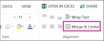
Select Merge & Center.

Important: When you merge multiple cells, the contents of only one cell (the upper-left cell for left-to-right languages, or the upper-right cell for right-to-left languages) appear in the merged cell. The contents of the other cells that you merge are deleted.

Unmerge cells

Select the Merge & Center down arrow.
Select Unmerge Cells.

Important:

You cannot split an unmerged cell. If you are looking for information about how to split the contents of an unmerged cell across multiple cells, see Distribute the contents of a cell into adjacent columns.
After merging cells, you can split a merged cell into separate cells again. If you don’t remember where you have merged cells, you can use the Find command to quickly locate merged cells.

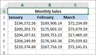
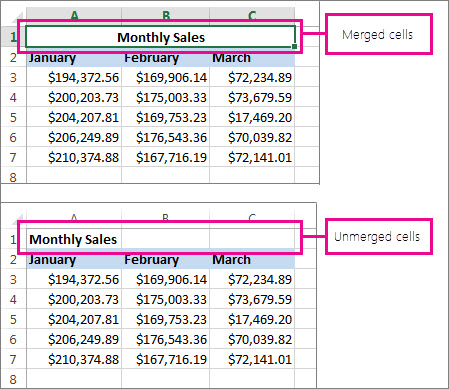
Merging combines two or more cells to create a new, larger cell. This is a great way to create a label that spans several columns.

In the example here, cells A1, B1, and C1 were merged to create the label “Monthly Sales” to describe the information in rows 2 through 7.

Merge cells

Merge two or more cells by following these steps:

Select two or more adjacent cells you want to merge.

Important: Ensure that the data you want to retain is in the upper-left cell, and keep in mind that all data in the other merged cells will be deleted. To retain any data from those other cells, simply copy it to another place in the worksheet—before you merge.
On the Home tab, select Merge & Center.

Tips:

If Merge & Center is disabled, ensure that you’re not editing a cell—and the cells you want to merge aren’t formatted as an Excel table. Cells formatted as a table typically display alternating shaded rows, and perhaps filter arrows on the column headings.
To merge cells without centering, click the arrow next to Merge and Center, and then click Merge Across or Merge Cells.

Unmerge cells

If you need to reverse a cell merge, click onto the merged cell and then choose Unmerge Cells item in the Merge & Center menu (see the figure above).

Split text from one cell into multiple cells

You can take the text in one or more cells, and distribute it to multiple cells. This is the opposite of concatenation, in which you combine text from two or more cells into one cell.

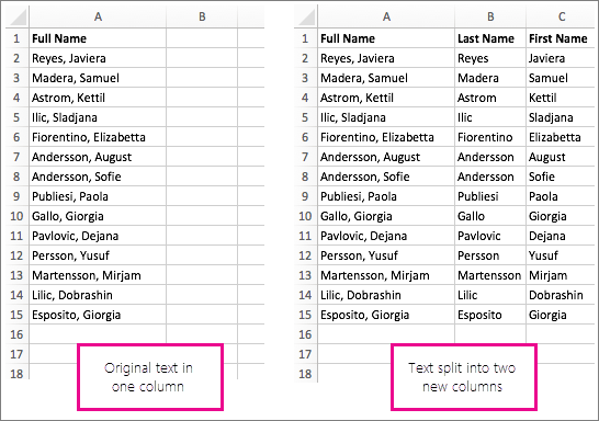
For example, you can split a column containing full names into separate First Name and Last Name columns:

Follow the steps below to split text into multiple columns:

Select the cell or column that contains the text you want to split.
Note: Select as many rows as you want, but no more than one column. Also, ensure that are sufficient empty columns to the right—so that none of your data is deleted. Simply add empty columns, if necessary.
Click Data >Text to Columns, which displays the Convert Text to Columns Wizard.
Click Delimited > Next.
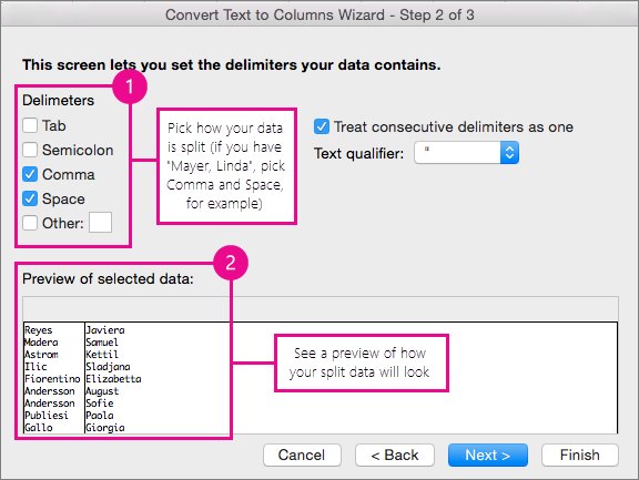
Check the Space box, and clear the rest of the boxes. Or, check both the Comma and Space boxes if that is how your text is split (such as «Reyes, Javiers», with a comma and space between the names). A preview of the data appears in the panel at the bottom of the popup window.
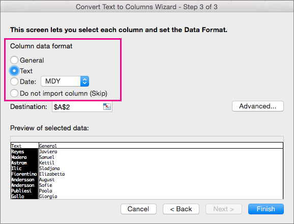
Click Next and then choose the format for your new columns. If you don’t want the default format, choose a format such as Text, then click the second column of data in the Data preview window, and click the same format again. Repeat this for all of the columns in the preview window.
Click the button to the right of the Destination box to collapse the popup window.
Anywhere in your workbook, select the cells that you want to contain the split data. For example, if you are dividing a full name into a first name column and a last name column, select the appropriate number of cells in two adjacent columns.
Click the button to expand the popup window again, and then click the Finish button.

Merging combines two or more cells to create a new, larger cell. This is a great way to create a label that spans several columns. For example, here cells A1, B1, and C1 were merged to create the label “Monthly Sales” to describe the information in rows 2 through 7.

Merge cells

Click the first cell and press Shift while you click the last cell in the range you want to merge.

Important: Make sure only one of the cells in the range has data.
Click Home > Merge & Center.

If Merge & Center is dimmed, make sure you’re not editing a cell or the cells you want to merge aren’t inside a table.

Tip: To merge cells without centering the data, click the merged cell and then click the left, center or right alignment options next to Merge & Center.

If you change your mind, you can always undo the merge by clicking the merged cell and clicking Merge & Center.

Unmerge cells

To unmerge cells immediately after merging them, press Ctrl + Z. Otherwise do this:

Click the merged cell and click Home > Merge & Center.

The data in the merged cell moves to the left cell when the cells split.

Need more help?

You can always ask an expert in the Excel Tech Community or get support in the Answers community.

Part 1# How To Merge Rows in Excel

When it comes to merging the Excel rows there are two ways that allow you to merge rows data easily.

Merge Excel rows using a formula
Combine multiple rows using the Merge Cells add-in

1. How to Merge Multiple Rows using Excel Formulas

Excel provides various formulas that help you combine data from different rows. Possibly the easiest one is the CONCATENATE function. So here checks out some examples for concatenating numerous rows into one:

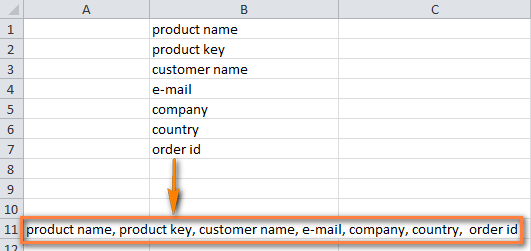
Merge rows with spaces between data: For example =CONCATENATE(B1,” “,B2,” “,B3)
Combine rows without any space between the values: For example =CONCATENATE(A1,A2,A3)
Merge rows > separate the values with comma: For Example =CONCATENATE(A1,”, “,A2,”, “,A3)

Now check how the CONCATENATE formula works on the real data.

On the sheet choose an empty cell and type the formula into it. Type the formula as per the data rows
And copy the formula across entire other cells in the row.

Now, simply you are having several data rows merged into one row.

2. How to Combine Rows in Excel using the Merge Cells Add-in

The Merge Cells add-in is used for merging various types of cells in Excel. This allows you to merges the individual cells and also combines data from entire rows or columns.

Please Note: You need to download a merge cell add-ins for third-party sites available online. Search in Google for add-ins.

Follow the given steps to combine two or more rows in your table:

Choose rows you are looking to merge > click on the Merge Cells icon.
Now the merge cells dialog window opens with a table or range selected already. And in the upper part of the window, you can see the three basic things:

- How you want to join cells – For combining rows of data > choose “column by column“.
- How to separate merged values with – an array of standard separators is available to choose from > comma, space, semicolon, and a line break. So select the separator as per your desire.
- Where you need to place the merged cells > either the top cell or bottom cell.

Now check the lower part of the Windows to check if you need any additional options:

- Clear the content of selected cells – Choose this if need data to remain in the merged cells only.
- Merge all areas in the selection – This option allows you to merge rows in two or more non-adjacent ranges.
- Skip empty cells and Wrap text – Well, these are self-explanatory.
- Lastly, Create a backup copy of the worksheet – This option is checked by default. It is just a precaution that keeps you on the safe side and prevents the risk of data loss.

Click the Merge button > to check the result – possible the merged rows of data separated by line breaks.

So, these are the two ways that allow you to merge rows in Excel without any data loss. Now, check out the ways on how to combine two columns in Excel.

Part 2# How To Merge Columns In Excel

Here check out the 3 ways to merge data from several columns into one without using VBA macro.

Merge two columns using formulas
Combine columns data via NotePad
The fastest way to join multiple columns

1. Merge Two Columns using Excel Formulas

1. Into your table > insert a new column > in the column header place the mouse pointer > right-click the mouse > select Insert from the context menu. Name the newly added columns for eg. – “Full Name”

2. In the cell D2, write the formula: =CONCATENATE(B2,” “,C2). The B2 and C2 are the addresses of First Name and Last Name. And in the formula, the quotation marks “” is the separator that will be inserted between merged names any other symbol can be used as a separator e.g. a comma.

3. Just like this, join data from several cells into one by making use of any separator of your choice.

4. Simply, copy the formula to other cells of the Full Name column. If the First name or the Last name is deleted, then the corresponding data in the Full name Column will also be gone.

5. Next, try converting the formula to a value so that you can remove the unnecessary columns from the Excel worksheet. Choose entire cells with data in the merged column (choose the first cell in “Full Name” Column > press Ctrl +Shift + Arrow Down)

6. Now copy the contents of the columns to clipboard > right click on the cell in the same column (“Full Name”) > choose “Paste Special” context menu > choose “Values” radio button > click OK.

7. Now remove “First Name” & “Last Name” columns that are not required. Click the column B header > press and hold Ctrl > click column C header.

8. After that make a right-click on any selected columns > select Delete from the context menu.

9. This is it, now you have successfully merged the names from 2 columns into one.

2. Combine columns Data via Notepad

This is another way that allows you to merge several columns. Here you don’t need any formulas. This is suitable for combining adjacent columns to make use of the same delimiter for all of them.

For Example: If looking for combining 2 columns with First Names and Last Names into one:

Choose both columns you need to merge: Click B1 > press Shift + ArrrowRight for choosing C1 > then hit Ctrl + Shift + ArrowDown for choosing entire data cells with data in two columns.

And copy data to clipboard > open Notepad > insert data from the clipboard to the Notepad

Then copy tab character to clipboard > hit Tab right in Notepad > hit Ctrl + Shift + LeftArrow > press Ctrl + X.
After that Replace Tab characters in Notepad with the separator, you require.
Hit Ctrl + H for opening the “Replace” dialog box > paste the Tab character from the clipboard in Find what field > type the separator Space, comma etc in “Replace with” field. Hit the Replace All button > to close the dialog box press Cancel

Now select the entire text in the Notepad and copy it to Clipboard.
Then switch back to Excel worksheet (press Alt + Tab) > choose B1 cell and paste text from Clipboard to your table.

And rename column B to “Full Name“ and remove the “Last name” column.

So, this is the second way that allows you to merge columns in Excel without any data loss.

3. Join Columns Using Merge Cells Add-in For Excel

This is the easiest and quickest way for combining data from numerous Excel columns into one. Just make use of the third party merge cells add-in for Excel.

And with the merge cells add-in you can merge data from many cells by using any separator you like (for example carriage return or line break). With this, you can join row by row, column by column, or merge data from the selected cell into one without any loss.

There are many third-party add-ins online sites that allow you to download the add-ins and merge the cells easily in just a few clicks.

Conclusion:

So this is all about merging rows and columns in Excel without any data loss.

Follow the given steps to combine text in rows and columns easily.

Hope the given different steps will allow you to perform the task easily in the rows and column. Here I have described different methods of merging rows and columns data in Excel without any data loss.

So make use of anyone that you find easy for you.

However if in case you come to face any issue or data loss situation in Excel then make use of the MS Excel Repair Tool. This is the best tool that allows you to repair and recover data from the corrupted, damaged Excel file.

Additionally, you can learn advanced Excel to become more productive and easily utilize Excel functions and formulas.

Priyanka is an entrepreneur & content marketing expert. She writes tech blogs and has expertise in MS Office, Excel, and other tech subjects. Her distinctive art of presenting tech information in the easy-to-understand language is very impressive. When not writing, she loves unplanned travels.

Источник

Download Article

Do you want to merge two columns in Excel without losing data? There are three easy ways to combine columns in your spreadsheet—Flash Fill, the ampersand (&) symbol, and the CONCAT function. Unlike merging cells, these options preserve your data and allow you to separate values with spaces and commas. This wikiHow guide will teach you how to combine columns in Microsoft Excel.

1
Know when to use Flash Fill. Flash Fill is the fastest way to combine the values of two columns (such as columns of separated first and last names). You’ll teach Flash Fill how to merge the data by typing the first merged cell yourself (e.g., FirstName LastName). Flash Fill will sense the pattern and fill out the rest of the column.^[1]
- The two columns you’re combining must be next to each other to use Flash Fill.
- Don’t use Flash Fill if any of the following is true for your data (use the ampersand symbol or the CONCAT function instead):
  - The columns you want to combine aren’t consecutive (e.g., combining columns A and F).
  - You want to be able to make changes to the original columns and have those change automatically update in the merged column.
2

Add a blank column next to the columns you want to combine. In this example, let’s say column A contains first names, column B contains last names, and that we want column C to contain first and last names combined. If column C isn’t blank right now, right click the C column header and select Insert from the menu.

Advertisement
3
Type the full name into the first cell in column C. For example, if A1 contains Joe and B1 contains Williams, type Joe Williams into C1.
- Flash Fill can detect all sorts of patterns. For example, if column A contains area codes and column B contains phone numbers, you could type the area code and phone number into column C.
- You can even separate the contents of the columns with words or symbols, as long as you don’t make the pattern too hard for Excel to understand. For example:
  - A1 contains the area code 212 and B1 contains 555-1212, you could type (212) 555-1212 into column C and Excel should sense the pattern.
4

Press ↵ Enter or ⏎ Return. This teaches Flash Fill the pattern.
5
Start typing the next combined name into C2. As you type, you’ll see that Excel suggest the next combination automatically.
- For example, if A2 is Maria and B2 is Martinez, Excel will suggest Maria Martinez.
6
Press ↵ Enter or ⏎ Return. This automatically combines the remaining cells from columns A and B into a single merged column C. You don’t even have to drag down a formula—the two columns are now merged into one.
- If the column does not fill, press Control + E on the keyboard to activate Flash Fill manually.
- You can safely delete the original two columns if you’d like. The new column doesn’t contain any formulas, so you won’t lose the merged data.

1
Click an empty cell near the columns you want to combine. This should be on the same row as the first row of data in the columns you’re combining.
- Using the Ampersand & is another easy way to combine two columns. You’ll create a simple formula using & symbols into the first cell, and then apply your formula to the rest of the data to merge the whole column.
2

Type an equals sign = into the blank cell. This begins the formula.
3

Click the first cell in the first column you want to join. For example, if you’re combining columns A and B, click A1. This adds the cell address to your formula.
4
Type &" ". Place a single space between the two quotation marks. This tells the formula to add a space between the contents of the two columns.^[2]
- For example, if column A contains first names and column B contains last names, the " " ensures a space between the first and last names in the new column (e.g., «Joe Williams» instead of «JoeWilliams.»
5

Type another &. This time, don’t add any quotes or spaces.
6
Click the first cell in the second column you want to merge. Now you’ll have a formula that looks something like this: =A1&" "&B1
- If you’d rather there not be a space between the words in the merged column, the formula would eliminate the » » and the second ampersand like this: =A1&B1
- You could also place a symbol, word, or phrase inside of the quotes if you want to insert something between the two joined cells.
7

Press ↵ Enter or ⏎ Return. You’ve now merged the contents of the two cells at the top of each column.
8
Click and drag the formula down the column. This merges the rest of the two columns.
- You can either click the cell and drag its bottom-right corner to the bottom of the columns, or double-click the square at the bottom-right corner of the cell to use autofill.
9
Convert the merged column into plain text. Because you used a formula to merge the two columns, the new column is just formulas, not text. If you want to delete the original columns and just keep the merged column, you’ll need to do this to avoid losing data:
- Select all the combined data you’ve created. For example, C1:C30.
- Press Control + C (PC) or Command + C (Mac) to copy it.
- Right-click the first cell in the column you just copied.
- Select Paste Special and choose Values.

1
Click an empty cell near the columns you want to combine. This should be on the same row as the first row of data in the columns you’re combining.
- CONCAT works just like using the ampersand symbol. Its advantage is that it’s easy to include in other formulas and is handy when making calculations.^[3] If you’re just joining two columns by hand, using the ampersand is much easier.
2
Type =CONCAT( into the blank cell. This begins the CONCAT formula.
- If you’re using a version of Excel from before 2019, use CONCATENATE instead of CONCAT.^[4]
3

Click the first cell in the first column you want to join. For example, if you’re combining columns A and B, click A1. This adds the cell address to your formula, which should now look something like this: =CONCAT(A1.
4
Type ," ",. Typing the first comma separates the first cell from " ", which adds a space between the two values. The second comma prepares you to select the second cell you’re merging.
- You should now have a formula that looks something like this: =CONCAT(A1," ",
5
Click the first cell in the second column you want to merge and type a closed parenthesis ). Now you’ll have a formula that looks something like this: =CONCAT(A1," ",B1).
- You could also place a symbol, word, or phrase inside of the quotes if you want to insert something between the two joined cells.
- Alternatively, if you want the merged text to appear without a space (e.g., JoeWilliams instead of Joe Williams), you could change the formula to =CONCAT(A1,B1).
6

Press ↵ Enter or ⏎ Return. This creates the formula and joins the two cells at the top of the columns.
7
Click and drag the formula down the column. This merges the rest of the two columns.
- You can either click the cell and drag its bottom-right corner to the bottom of the columns, or double-click the square at the bottom-right corner of the cell to use autofill.
8
Convert the merged column into plain text. Because you used a formula to merge the two columns, the new column is just formulas, not text. If you want to delete the original columns and just keep the merged column, you’ll need to do this to avoid losing data:
- Select all the combined data you’ve created. For example, C1:C30.
- Press Control + C (PC) or Command + C (Mac) to copy it.
- Right-click the first cell in the column you just copied.
- Select Paste Special and choose Values.

Ask a Question

200 characters left

Include your email address to get a message when this question is answered.

Submit

Thanks for submitting a tip for review!

References

About This Article

Article SummaryX

1. Add a blank column to the right of the two columns you’re merging.
2. Use Flash Fill to manually type the first combined cell and automatically fill the rest.
3. Use the & or CONCAT function to create a formula that joins any two columns.

Did this summary help you?

Thanks to all authors for creating a page that has been read 20,591 times.

Is this article up to date?

Источник

We can merge values in two or more cells in Excel. We can apply the same for columns as well. We are required to use the formula in every column cell by dragging or copy-paste the formula in each column. For example, we have a list of candidates with the first name in one column and the last name in another. The requirement here is to get the full name of all candidates in one column. We can do this by merging the column in Excel.

Excel Column Merge
- How to Merge Multiple Columns in Excel?
  - Method #1 – Using the CONCAT Function
    - Example #1
  - Method #2 – Merge the Cells by Using the “&” Symbol
    - Example #2
    - Example #3
    - Example #4
    - Example #5
- Things to Remembered
- Recommended Articles

How to Merge Multiple Columns in Excel?

We can merge the cells using two ways.

You can download this Column Merge Excel Template here – Column Merge Excel Template

Method #1 – Using the CONCAT Function

We can merge the cells using the CONCAT FunctionThe CONCATENATE function in Excel helps the user concatenate or join two or more cell values which may be in the form of characters, strings or numbers.read more. Let us see the below example.

Example #1

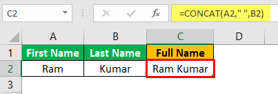
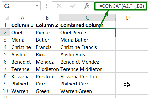
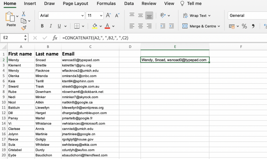
We have Ram and Kumar in the last name column in the first name column. Now, we need to merge the value in the full name column. So here we use =CONCAT(A2,” “,B2). The result will be as below.

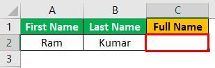
We have noticed that we have used” “between the A2 and B2. That is used to give space between the first name and last name. If we had not used” “in the function, the result would have been Ramkumar, which looks awkward.

Method #2 – Merge the Cells by Using the “&” Symbol

We can merge the cells using the “&” symbol with the CONCAT function. Let us see the example below.

Example #2

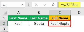
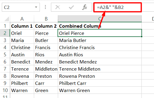
We can merge the cells by using the “&” symbol in the formula. So, let us combine the cells by using the “&” symbol. So, the formula will be =A2& “” &B2. The result will be Kapil Gupta.

Let us merge the value into two columns.

Example #3

We have a list of first and last names in two columns, A and B, below. Now, we require the full name in column C.

Follow the below steps:

We must place the cursor on C2.
Then, we must insert formula =CONCAT(A2,” ”,B2) in the C2 cell.
Next, we will copy cell C2 and paste it in the range of column C, i.e., if we have the first name and last name till the 11th row, then paste the formula till C11.

The result will be as shown below.

Example #4

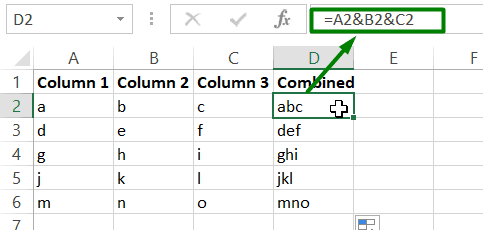
Suppose we have a list of 10 students whose first name, middle name, and last name are in columns A, B, and C, and we need the full name in column D.

Follow the below steps:

We must first place the cursor on D2.
Then, we need to put the formula =CONCAT(A2,” “,B2,” “,C2) in D2.
Then, we must copy the cell D2 and paste it in the range of column D., i.e., if we have the first name and last name till the 11th row, then paste the formula till D11.

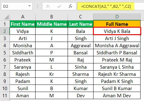
The result will look as shown in the below image.

Example #5

We have a list of first and last names in two columns, A and B, below. Next, we need to create a user ID for each person.

Note: Space is not allowed in a user ID.

Follow the below steps:

Firstly, we must place the cursor on C2.
Secondly, we should put the formula =CONCAT(A2,”.”,B2) in C2.
Lastly, we must copy cell C2 and paste it in the range of column C., i.e., suppose we have the first name and last name till the 11th row, then paste the formula till D11.

The result will look as shown in the below image. Similarly, we can merge the value using some other character, i.e. (dot (.), hyphen (-), the asterisk (*), etc.

Things to Remembered

CONCAT function works with Excel 2016 or above version. If we are working on the earlier version of Excel, we need to use the CONCATENATE function.
It is not mandatory to use any space or special character while merging the cells. We can merge the cells in excelMerging a cell in excel refers to combining two or more adjacent cells either vertically, horizontally or both ways. Merging excel cells is specifically required when a heading or title has to be centered over an area of a worksheet.read more or columns without using anything.

How to Combine Columns in Excel Sheets?

Let’s say, for example, you have two separate columns containing the first and last names of your customers. Now, you want to combine these two columns into a single column that contains the full names of the customers.

How to Combine Two Columns in Excel?

There are two methods to go about doing this. You can either use the CONCAT formula method or use the ampersand method. Both of these methods are equally easy to use and I’ll break them down one by one in the following sections.

How to Combine Two Columns in Excel with the CONCAT Function?

Click on the destination cell where you want to combine the two columns.

Enter the formula: =CONCAT(Column 1 Cell, Column 2 Cell).

Here, replace Column 1 Cell with the name of the first cell of column 1 and Column 2 cell

with the name of the first cell of column 2.

In this example, it is going to look like this: =CONCAT(A2,B2)

CONCAT Formula to Combine two columns in Excel

Enter the CONCAT formula in the third column and drag it to the end of the data range

Drag the formula to the entire cell range, as long as you need to.

How to Combine Two Columns in Excel with the Ampersand Symbol?

Click on the destination cell where you want the combined columns to appear.

Enter the formula, in this format =Column Cell 1&Column Cell 2

Here, replace Column 1 Cell with the name of the first cell of column 1 and Column 2 cell

with the name of the first cell of column 2.

In this example, it is going to look like this: =A2&B2

Enter the formula in the third column and drag till the end of the data range

Drag the formula to the data entire range.

Also Read:

Excel Conditional Formatting -the Best Guide (Bonus Video)

The Best Excel Project Management Template In 2021

How To Use Excel Countifs: The Best Guide

How to Combine Multiple Columns in Excel into One Column?

If you want to combine multiple columns in Excel into one column using the above two methods, follow these steps:

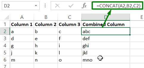
If you are using the CONCAT formula, keep adding the cell references from the extra columns inside the formula. For example, if you want to combine the column C along with columns A and B, the formula would be this: =CONCAT(A2, B2, C2)

Combine multiple columns in Excel using CONCAT

If you are using the ampersand method, keep adding the new cell references in the same format. For example, if you want to combine column C along with columns A and B, the formula would be this: =A2&B2&C2

Combine multiple columns in Excel using ampersand

How to Format Combined Columns in Excel?

While the above methods have technically combined the columns, their results are not always accurate. Let’s use the combined full names from the previous example. Let’s say that the first name and last name are not separated by a space. In this section, I’ll show you how to avoid such errors while combining columns in Excel.

How to Insert a Space Between Combined Cells of the Columns?

To insert a space between two cells of the combined columns, just add a dummy space between the cell references in the formula using the character: “ “

For example, if you are using the CONCAT function, it will look like this:

=CONCAT(A2,“ ”,B2)

Insert a space between two columns inside the CONCAT formula

Similarly, If you are using the ampersand method, your formula should look like this:

=A2&“ ”&B2

Insert a space between the two columns using the ampersand method

How to Correctly Display Dates and Currency in Combined Cells?

If the columns you combine contain any special formatting like dates, currency, or accounting, Excel will automatically strip the formatting before it combines the columns.

Excel removes special formatting of dates, currency etc before combining two columns

To avoid this, you can use the TEXT function to convert this special formatting into text before combining them together.

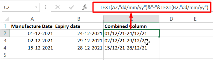
For example, if you want to combine two dates together to form a date range, use either one of the following formulas:

=TEXT(A2,”dd/mm/yy”)&”-“&TEXT(B2,”dd/mm/yy”)

How to keep the date formatting while combining columns using the ampersand method?

=CONCAT(TEXT(A2,”dd/mm/yy”),”-“,TEXT(B2,”dd/mm/yy”))

How to keep the date formatting while combining columns using the CONCAT formula?

In this example, A2 and B2 contain the original dates in proper date format.

How to Add Additional Text in Combined Cells?

Sometimes, you may need to add additional text in between or after the combined cells. To do this, follow the same technique you followed when you added spaces. Insert your custom text in between double quotes.

For example, if you want to add the phrase “was born on” in-between names and date of birth columns, you can use either one of these two formulas:

=CONCAT(A2,” expires on “,TEXT(B2,”dd/mm/yy”))

How to add additional text while combining columns using the CONCAT formula?

=TEXT(A2,”dd/mm/yy”)&”-“&TEXT(B2,”dd/mm/yy”)

How to add additional text while combining columns using the ampersand method?

How to Remove the Formula from the Combined Columns?

The combined column that you created, using the above methods is going to be dynamic. That means any change in the original values will affect the values in the combined column. To prevent this, copy the values of the combined column and paste them as values in the same column, or even a different column.

How to Merge Columns in Excel?

If you don’t want to combine the values of two columns, but want to just merge two columns into one instead, you can follow these steps:

Select the cells or columns that you want to merge.
Click on the “Merge & Centre” option on the “Home” tab.

Excel will merge the selected columns into one column.

Note: Please keep in mind that this will only keep the value from the upper-left corner cell and clear all other values.

Suggested Reads:

Excel Sumifs & Sumif Functions – The No.1 Complete Guide

Create An Excel Dashboard In 5 Minutes – The Best Guide

Dynamic Dropdown Lists In Excel – Top Data Validation Guide

Closing Thoughts

That’s all folks. In this guide, I have shown you how to combine two columns in Excel using the easiest methods. Try using these methods in a practice worksheet and let us know if you have any questions about it.

Want more high-quality guides for Excel? Check out our free Excel resources centre.

Click here to access in-depth Excel training courses and master in-demand advanced Excel skills.

Simon Sez IT has been teaching critical IT software for over ten years. For a low, monthly fee you can get access to 100+ IT training courses by seasoned professionals.

Simon Calder

Chris “Simon” Calder was working as a Project Manager in IT for one of Los Angeles’ most prestigious cultural institutions, LACMA.He taught himself to use Microsoft Project from a giant textbook and hated every moment of it. Online learning was in its infancy then, but he spotted an opportunity and made an online MS Project course — the rest, as they say, is history!

Источник

Are you having difficulty merging two or more Excel columns? Knowing how to combine multiple columns in Excel without losing data is a handy time-saver that allows you to consolidate your data and make your sheet look neater.

First and foremost, you should know that there are multiple ways you can merge data from two or more columns in Excel. Before we get started exploring these different ways, let’s start with a key step that helps the process — how to merge cells in Excel.

If you want to combine Google Sheets data, you can do that easily using Layer. Layer is a free add-on that allows you to share sheets or ranges of your main spreadsheet with different people. On top of that, you get to monitor and approve edits and changes made to the shared files before they’re merged back into your master file, giving you more control over your data.

Install the Layer Google Sheets Add-On today and Get Free Access to all the paid features, so you can start managing, automating, and scaling your processes on top of Google Sheets!

How to Combine Multiple Cells or Columns in Excel Without Losing Data?

Once you have merging cells under your belt, learning how to combine multiple Excel columns into one column becomes intuitive.

Whether you’re learning how to combine two cells in Excel, or ten, one of the main benefits of merging is that the formulae don’t change. Here are the following ways you can combine cells or merge columns within your Excel:

Use Ampersand (&) to merge two cells in Excel

If you want to know how to merge two cells in Excel, here’s the quickest and easiest way of doing so without losing any of your data.

1. Double-click the cell in which you want to put the combined data and type =
2. Click a cell you want to combine, type &, and click the other cell you wish to combine. If you want to include more cells, type &, and click on another cell you wish to merge, etc.
3. Press Enter when you have selected all the cells you want to combine

While this is useful for quickly merging data into a single cell, the merged data will not be formatted. This can make data untidy or challenging to read in some instances (e.g. full names or addresses).

If you want to add punctuation or spaces (delimiters), follow the below steps. For this example, let’s put a comma and a space between the first and last name as you would see on a registration list:

1. Double-click the cell in which you want to put the merged data and type =
2. Click a cell you want to merge
3. This time, type &”, ”& before you click the next cell you want to merge. If you want to include more cells, type &”, ”& before clicking the next cell you want to merge, etc.
4. Press Enter when you have selected all the cells you want to combine

As you can see, now your merged data comes out in a neater format, with each piece of data appropriately separated.

Use the CONCATENATE function to merge multiple columns in Excel

This method is similar to the ampersand method, and also allows you to format your merged data. First, you need to use the CONCATENATE function to merge a row of cells:

1. Insert the =CONCATENATE function as laid out in the instructions above
2. Type in the references of the cells you want to combine, separating each reference with ,», «, (e.g. B2,», «,C2,», «,D2). This will create spaces between each value.
3. Press Enter

Now that you have successfully merged your cells, you can follow these simple steps to merge multiple columns:

1. Hover your mouse over the bottom-right corner of the merged cell you just created
2. When the cursor changes into a + symbol, drag your cursor as far down the column as you want and release it

Once you release the mouse, you should see that your merged cell has become a merged column, containing all of the data from your chosen columns.

*The CONCAT function is another formula used for combining data from different cells. However, it is limited to two references and does not allow you to include delimiters.

Use the TEXTJOIN function to merge multiple columns in Excel

This method works only with Excel 365, 2021, and 2019. As you can probably tell, this function is helpful when you want to combine two or more text cells in Excel.

The following steps will show you how to use the TEXTJOIN function, once again using the comma and space combination to create your first merged cell:

1. Double-click the cell in which you want to put the combined data
2. Type =TEXTJOIN to insert the function
3. Type “, ”,TRUE, followed by the references of the cells you want to combine, separating each reference with a comma (the role of TRUE is to disregard empty cells you may have input)
4. Press Enter

In order to create the rest of your combined column, use the drag-and-drop steps listed below:

1. Hover your mouse over the bottom-right corner of the merged cell you just created
2. When the cursor changes into a + symbol, drag your cursor as far down the column as you want and release it.

Now your columns of data have successfully merged into your new column.

The Beginner’s Guide to Excel Version Control

Discover what Excel version control is, the version control features Excel has to offer, and how to use them to share, merge, and review Excel changes

Use the INDEX formula to stack multiple columns into one column in Excel

Let’s say you want to create a stack of data from your multiple columns, rather than create a single cell. You can easily do this across multiple cells and columns within your spreadsheet using the INDEX formula:

1. Select all of the cells containing your data
2. Type in a name for this group of data in the “Name Box” (box located to the left side of the formula bar). In this example, I’ve named the data “_my_data”
3. Select an empty cell in your Excel sheet where you want your stacked data to be located. Input the following INDEX formula (remember to substitute with your data name):

=INDEX(_my_data,1+INT((ROW(A1)-1)/COLUMNS(_my_data)),MOD(ROW(A1)-1+COLUMNS(_my_data),COLUMNS(_my_data))+1)

4. The first value from your data range should appear. Hover over the cell until the cursor changes into a + symbol, and drag your cursor as far down until you receive a #REF! value (this signals the end of your data set)

Other ways to combine multiple columns in Excel: Notepad and VBA script

There are two other ways you can combine multiple columns in Excel. These are often more time-consuming, and use other tools as part of the process. However, they may be more helpful for users who wish to avoid using Excel formulae.

Use Notepad to merge multiple columns in Excel

You can use Notepad to extract, format, and replace your data from multiple columns in your Excel. For this, you need to copy and paste each column from your Excel sheet into a Notepad file. Then, use the Replace function to add commas between each value. Once finished, you can copy and paste your formatted data back into your Excel.

Use VBA script to combine two or more columns in Excel

As an alternative to the INDEX function stacking method, you can use VBA script. Simply right-click and select “View code” within your Excel, and copy and paste the code in a new window. Press “F5” to run the code and create a Macro. You can then apply this to your Excel by selecting your data range and applying it to your destination column.

Want to Boost Your Team’s Productivity and Efficiency?

Transform the way your team collaborates with Confluence, a remote-friendly workspace designed to bring knowledge and collaboration together. Say goodbye to scattered information and disjointed communication, and embrace a platform that empowers your team to accomplish more, together.

Key Features and Benefits:

Centralized Knowledge: Access your team’s collective wisdom with ease.
Collaborative Workspace: Foster engagement with flexible project tools.
Seamless Communication: Connect your entire organization effortlessly.
Preserve Ideas: Capture insights without losing them in chats or notifications.
Comprehensive Platform: Manage all content in one organized location.
Open Teamwork: Empower employees to contribute, share, and grow.
Superior Integrations: Sync with tools like Slack, Jira, Trello, and more.

Limited-Time Offer: Sign up for Confluence today and claim your forever-free plan, revolutionizing your team’s collaboration experience.

Conclusion

As you can see, combining multiple columns is easy in Excel. Whether you’re combing multiple Excel files, or columns and cells, there are a variety of ways that cater to different users, depending on their technical abilities or needs.

As a result, not only can you format your Excel into a cohesive and seamless spreadsheet, but also save time and optimize your productivity when evaluating, managing, or sharing important data. Once you know how to combine multiple columns in Excel into one column, combining or merging your data can become one quick and simple task.

Источник

If you’re using Excel and have data split across multiple columns that you want to combine, you don’t need to manually do this. Instead, you can use a quick and easy formula to combine columns.

We’re going to show you how to combine two or more columns in Excel using the ampersand symbol or the CONCAT function. We’ll also offer some tips on how to format the data so that it looks exactly how you want it.

How to Combine Columns in Excel

There are two methods to combine columns in Excel: the ampersand symbol and the concatenate formula. In many cases, using the ampersand method is quicker and easier than the concatenate formula. That said, use whichever you feel most comfortable with.

1. How to Combine Excel Columns With the Ampersand Symbol

Click the cell where you want the combined data to go.
Type =
Click the first cell you want to combine.
Type &
Click the second cell you want to combine.
Press the Enter key.

For example, if you wanted to combine cells A2 and B2, the formula would be: =A2&B2

2. How to Combine Excel Columns With the CONCAT Function

Click the cell where you want the combined data to go.
Type =CONCAT(
Click the first cell you want to combine.
Type ,
Click the second cell you want to combine.
Type )
Press the Enter key.

For example, if you wanted to combine cell A2 and B2, the formula would be: =CONCAT(A2,B2)

This formula used to be CONCATENATE, rather than CONCAT. Using the former works to combine two columns in Excel, but it is depreciating, so you should use the latter to ensure compatibility with current and future Excel versions.

How to Combine More Than Two Excel Cells

You can combine as many cells as you want using either method. Simply repeat the formatting like so:

=A2&B2&C2&D2 … etc.
=CONCAT(A2,B2,C2,D2) … etc.

How to Combine the Entire Excel Column

Once you have placed the formula in one cell, you can use this to automatically populate the rest of the column. You don’t need to manually type in each cell name that you want to combine.

To do this, double-click the bottom-right corner of the filled cell. Alternatively, left-click and drag the bottom-right corner of the filled cell down the column. It’s an Excel AutoFill trick to build spreadsheets faster.

Tips on How to Format Combined Columns in Excel

Your combined Excel columns could contain text, numbers, dates, and more. As such, it isn’t always suitable to leave the cells combined without formatting them.

To help you out, here are various tips on how to format combined cells. In our examples, we’ll refer to the ampersand method, but the logic is the same for the CONCAT formula.

1. How to Put a Space Between Combined Cells

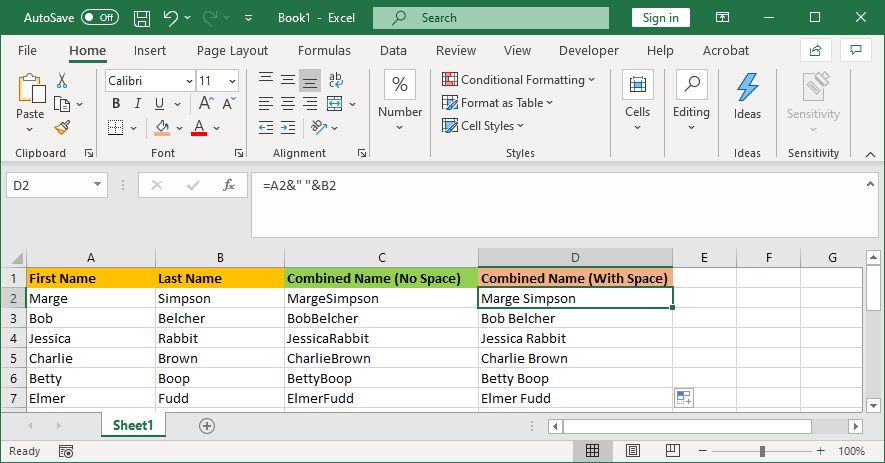
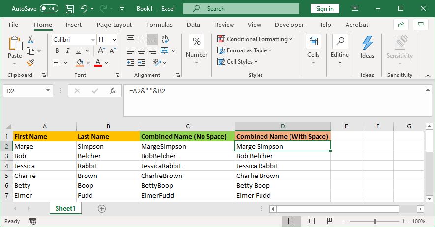
If you had a «First name» column and a «Last name» column, you would want a space between the two cells.

To do this, the formula would be: =A2&» «&B2

This formula says to add the contents of A2, then add a space, then add the contents of B2.

It doesn’t have to be a space. You can put whatever you want between the speech marks, like a comma, a dash, or any other symbol or text.

2. How to Add Additional Text Within Combined Cells

The combined cells don’t just have to contain their original text. You can add whatever additional information you want.

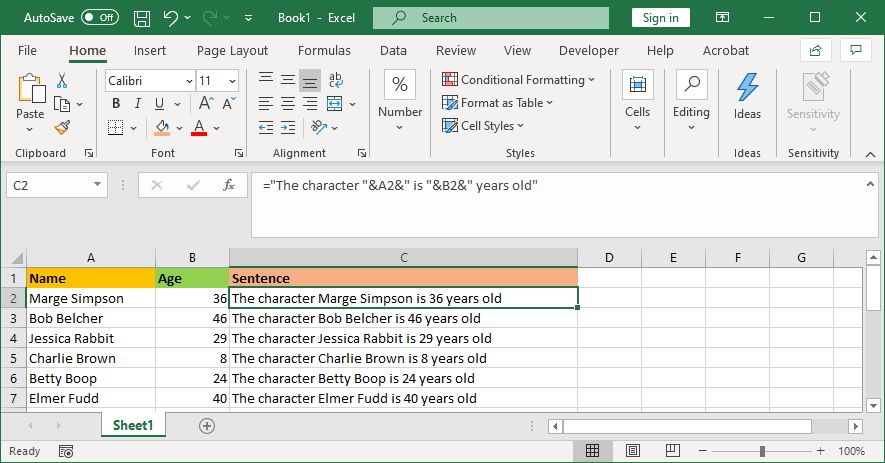
Let’s say cell A2 contains someone’s name (e.g., Marge Simpson) and cell B2 contains their age (e.g., 36). We can build this into a sentence that reads «The character Marge Simpson is 36 years old».

To do this, the formula would be: =»The character «&A2&» is «&B2&» years old»

The additional text is wrapped in speech marks and followed by an &. You don’t need to use speech marks when referencing a cell. Remember to include where the spaces should go; so «The character » with a space at the end.

3. How to Correctly Display Numbers in Combined Cells

If your original cells contain formatted numbers like dates or currency, you’ll notice that the combined cell strips the formatting.

You can solve this with the TEXT function, which you can use to define the required format.

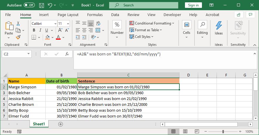
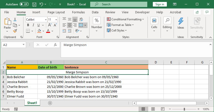
Let’s say cell A2 contains someone’s name (e.g., Marge Simpson) and cell B2 contains their date of birth (e.g., 01/02/1980).

To combine them, you might think to use this formula: =A2&» was born on «&B2

However, that’ll output: Marge Simpson was born on 29252. That’s because Excel converts the correctly formatted date of birth into a plain number.

By applying the TEXT function, you can tell Excel how you want the merged cell to be formatted. Like so: =A2&» was born on «&TEXT(B2,»dd/mm/yyyy»)

That’s slightly more complicated than the other formulas, so let’s break it down:

=A2 — merge cell A2.
&» was born on « — add the text «was born on» with a space on both sides.
&TEXT — add something with the text function.
(B2,»dd/mm/yyyy») — merge cell B2, and apply the format of dd/mm/yyyy to the contents of that field.

You can switch out the format for whatever the number requires. For example, $#,##0.00 would show currency with a thousand separator and two decimals, # ?/? would turn a decimal into a fraction, H:MM AM/PM would show the time, and so on.

You can find more examples and information on the Microsoft Office TEXT function support page.

How to Remove the Formula From Combined Columns

If you click a cell within the combined column, you’ll notice that it still contains the formula (e.g., =A2&» «&B2) rather than the plain text (e.g., Marge Simpson).

This isn’t a bad thing. It means that whenever the original cells (e.g., A2 and B2) are updated, the combined cell will automatically update to reflect those changes.

However, it does mean that if you delete the original cells or columns then it will break your combined cells. As such, you might want to remove the formula from the combined column and make it plain text.

To do this, right-click the header of the combined column to highlight it, then click Copy.

Next, right-click the header of the combined column again—this time, beneath Paste Options, select Values. Now the formula is gone, leaving you with plain text cells that you can edit directly.

How to Merge Columns in Excel

Instead of combining columns in Excel, you can also merge them. This will turn multiple horizontal cells into one cell. Merging cells only keeps the values from the upper-left cell and discards the rest.

To do this, select the cells or columns that you want to merge. In the Ribbon, on the Home tab, click the Merge & Center button (or use the dropdown arrow next to it).

For more information on this, read our article on how to merge and unmerge cells in Excel. You can also merge entire Excel sheets and files together.

Save Time When Using Excel

Now you know how to combine columns in Excel. You can save yourself lots of time—you don’t need to combine them by hand. It’s just one of the many ways that you can use formulas to speed up common tasks in Excel.

Источник

Merge cells

Unmerge cells

Merge cells

Unmerge cells

Split text from one cell into multiple cells

Merge cells

Unmerge cells

Need more help?

See Also

Need more help?

Part 1# How To Merge Rows in Excel

1. How to Merge Multiple Rows using Excel Formulas

2. How to Combine Rows in Excel using the Merge Cells Add-in

Part 2# How To Merge Columns In Excel

1. Merge Two Columns using Excel Formulas

2. Combine columns Data via Notepad

3. Join Columns Using Merge Cells Add-in For Excel

Conclusion:

References

About This Article

Is this article up to date?

Table of contents

How to Merge Multiple Columns in Excel?

Method #1 – Using the CONCAT Function

Example #1

Method #2 – Merge the Cells by Using the “&” Symbol

Example #2

Example #3

Example #4

Example #5

Things to Remembered

Recommended Articles

How to Combine Columns in Excel Sheets?

How to Combine Two Columns in Excel with the CONCAT Function?

How to Combine Two Columns in Excel with the Ampersand Symbol?

How to Combine Multiple Columns in Excel into One Column?

How to Format Combined Columns in Excel?

How to Insert a Space Between Combined Cells of the Columns?

How to Correctly Display Dates and Currency in Combined Cells?

How to Add Additional Text in Combined Cells?

How to Remove the Formula from the Combined Columns?

How to Merge Columns in Excel?

Closing Thoughts

Simon Calder

How to Combine Multiple Cells or Columns in Excel Without Losing Data?

Use Ampersand (&) to merge two cells in Excel

Use the CONCATENATE function to merge multiple columns in Excel

Use the TEXTJOIN function to merge multiple columns in Excel

The Beginner’s Guide to Excel Version Control

Use the INDEX formula to stack multiple columns into one column in Excel

Other ways to combine multiple columns in Excel: Notepad and VBA script

Use Notepad to merge multiple columns in Excel

Use VBA script to combine two or more columns in Excel

Want to Boost Your Team’s Productivity and Efficiency?

Conclusion

How to Combine Columns in Excel

1. How to Combine Excel Columns With the Ampersand Symbol

2. How to Combine Excel Columns With the CONCAT Function

How to Combine More Than Two Excel Cells

How to Combine the Entire Excel Column

Tips on How to Format Combined Columns in Excel

1. How to Put a Space Between Combined Cells

2. How to Add Additional Text Within Combined Cells

3. How to Correctly Display Numbers in Combined Cells

How to Remove the Formula From Combined Columns

How to Merge Columns in Excel

Save Time When Using Excel