Excel and inside if you - Word и Excel - помощь в работе с программами

Содержание

IF function
Simple IF examples
Common problems
Need more help?
Multiple IFs in Excel
Multiple IF Conditions in Excel
Explanation
Examples
Example #1
Example #2
Example #3
Example #4
Things to Remember
Recommended Articles
Using IF with AND, OR and NOT functions
Examples
Using AND, OR and NOT with Conditional Formatting
Need more help?
See also

IF function

The IF function is one of the most popular functions in Excel, and it allows you to make logical comparisons between a value and what you expect.

So an IF statement can have two results. The first result is if your comparison is True, the second if your comparison is False.

For example, =IF(C2=”Yes”,1,2) says IF(C2 = Yes, then return a 1, otherwise return a 2).

Use the IF function, one of the logical functions, to return one value if a condition is true and another value if it’s false.

IF(logical_test, value_if_true, [value_if_false])

The condition you want to test.

The value that you want returned if the result of logical_test is TRUE.

The value that you want returned if the result of logical_test is FALSE.

Simple IF examples

In the above example, cell D2 says: IF(C2 = Yes, then return a 1, otherwise return a 2)

In this example, the formula in cell D2 says: IF(C2 = 1, then return Yes, otherwise return No)As you see, the IF function can be used to evaluate both text and values. It can also be used to evaluate errors. You are not limited to only checking if one thing is equal to another and returning a single result, you can also use mathematical operators and perform additional calculations depending on your criteria. You can also nest multiple IF functions together in order to perform multiple comparisons.

B2,”Over Budget”,”Within Budget”)» loading=»lazy»>

=IF(C2>B2,”Over Budget”,”Within Budget”)

In the above example, the IF function in D2 is saying IF(C2 Is Greater Than B2, then return “Over Budget”, otherwise return “Within Budget”)

B2,C2-B2,»»)» loading=»lazy»>

In the above illustration, instead of returning a text result, we are going to return a mathematical calculation. So the formula in E2 is saying IF(Actual is Greater than Budgeted, then Subtract the Budgeted amount from the Actual amount, otherwise return nothing).

In this example, the formula in F7 is saying IF(E7 = “Yes”, then calculate the Total Amount in F5 * 8.25%, otherwise no Sales Tax is due so return 0)

Note: If you are going to use text in formulas, you need to wrap the text in quotes (e.g. “Text”). The only exception to that is using TRUE or FALSE, which Excel automatically understands.

Common problems

What went wrong

There was no argument for either value_if_true or value_if_False arguments. To see the right value returned, add argument text to the two arguments, or add TRUE or FALSE to the argument.

This usually means that the formula is misspelled.

Need more help?

You can always ask an expert in the Excel Tech Community or get support in the Answers community.

Источник

Multiple IFs in Excel

Multiple IF Conditions in Excel

The multiple IF conditions in Excel are IF statements contained within another IF statement. They are used to test multiple conditions simultaneously and return distinct values. The additional IF statements can be included in the “value if true” and “value if false” arguments of a standard IF formula.

For example, suppose we have a dataset of students’ scores from B1:B12. We need to grade the students according to their scores. Then, using the IF condition, we can manage the multiple conditions. In this example, we can insert the nested IF formula in cell D1 to assign a grade to a score. We can grade total score as “A,” “B,” “C,” “D,” and “F.” A score would be “F” if it is greater than or equal to 30, “D” if it is greater than 60, and “C” if it is greater than or equal to 70, and “A,” “B” if the score is less than 95. We can insert the formula in D1 with 5 separate IF functions:

Explanation

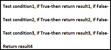
The IF formula is used when we wish to test a condition and return one value if the condition is met and another value if it is not met.

Syntax

IF (condition1, result1, IF (condition2, result2, IF (condition3, result3,………..)))

Examples

Example #1

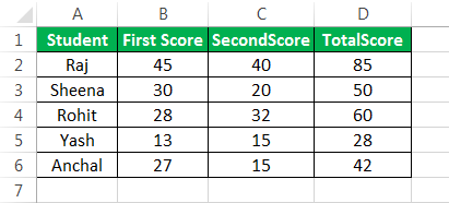
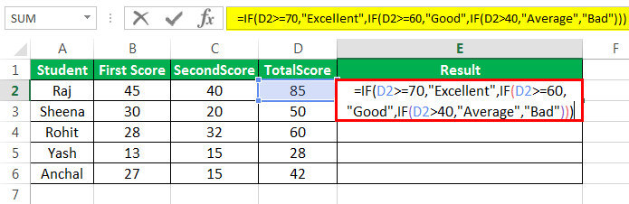
Suppose we wish to find how a student scores in an exam. There are two exam scores of a student, and we define the total score (sum of the two scores) as “Good,” “Average,” and “Bad.” A score would be “Good” if it is greater than or equal to 60, ‘Average’ if it is between 40 and 60, and ‘Bad’ if it is less than or equal to 40.

Let us say the first score is stored in column B, the second in column C.

The following formula tells Excel to return “Good,” “Average,” or “Bad”:

=IF(D2>=60,”Good”,IF(D2>40,”Average”,”Bad”))

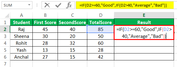
This formula returns the result as given below:

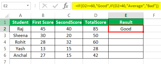
Drag the formula to get results for the rest of the cells.

We can see that one multiple IF function is sufficient in this case as we need to get only 3 results.

Example #2

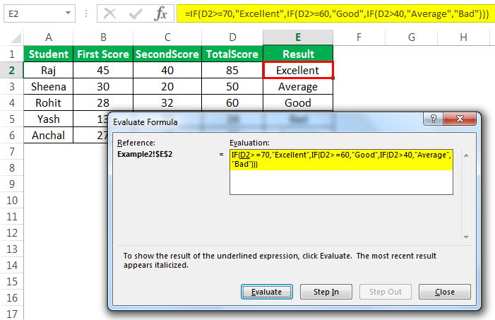
We want to test one more condition in the above examples: the total score of 70 and above is categorized as “Excellent.”

=IF(D2>=70,”Excellent”,IF(D2>=60,”Good”,IF(D2>40,”Average”,”Bad”)))

This formula returns the result as given below:

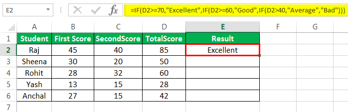
Excellent: >=70

Good: Between 60 & 69

Average: Between 41 & 59

Bad:

We can add several “IF” conditions if required similarly.

Example #3

Suppose we wish to test a few sets of different conditions. In that case, those conditions can be expressed using logical OR and AND, nesting the functions inside IF statements and then nesting the IF statements into each other.

For instance, if we have two columns containing the number of targets made by an employee in 2 quarters: Q1 and Q2. Then, we wish to calculate the performance bonus of the employee based on a higher target number.

We can make a formula with the logic:

If either Q1 or Q2 targets are greater than 70, then the employee gets a 10% bonus,

If either of them is greater than 60, then the employee receives a 7% bonus,

If either of them is greater than 50, then the employee gets a 5% bonus,

If either is greater than 40, then the employee receives a 3% bonus. Else, no bonus.

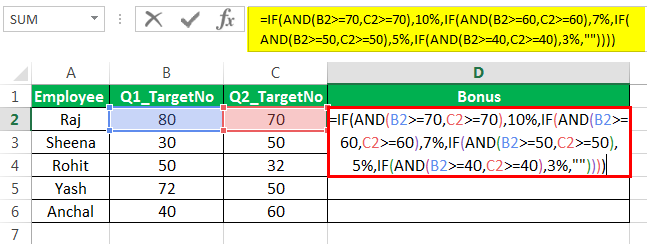
So, we first write a few OR statements like (B2>=70,C2>=70), and then nest them into logical tests of IF functions as follows:

=IF(OR(B2>=70,C2>=70),10%,IF(OR(B2>=60,C2>=60),7%, IF(OR(B2>=50,C2>=50),5%, IF(OR(B2>=40,C2>=40),3%,””))))

This formula returns the result as given below:

Next, drag the formula to get the results of the rest of the cells.

Example #4

Now, let us say we want to test one more condition in the above example:

If both Q1 and Q2 targets are greater than 70, then the employee gets a 10% bonus

if both of them are greater than 60, then the employee receives a 7% bonus

if both of them are greater than 50, then the employee gets a 5% bonus

if both of them are greater than 40, then the employee receives a 3% bonus

Else, no bonus.

So, we first write a few AND statements like (B2>=70,C2>=70), and then nest them: tests of IF functions as follows:

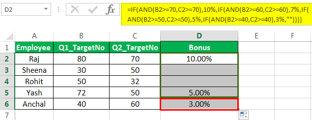
=IF(AND(B2>=70,C2>=70),10%,IF(AND(B2>=60,C2>=60),7%, IF(AND(B2>=50,C2>=50),5%, IF(AND(B2>=40,C2>=40),3%,””))))

This formula returns the result as given below:

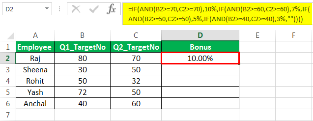
Next, drag the formula to get results for the rest of the cells.

Things to Remember

The multiple IF function evaluates the logical tests in the order they appear in a formula. So, for example, as soon as one condition evaluates to be “True,” the following conditions are not tested.

For instance, if we consider the second example discussed above, the multiple IF condition in Excel evaluates the first logical test (D2>=70) and returns “Excellent” because the condition is “True” in the below formula:

=IF(D2>=70,”Excellent”,IF(D2>=60,,”Good”,IF(D2>40,”Average”,”Bad”))

Now, if we reverse the order of IF functions in Excel as follows:

=IF(D2>40,”Average”,IF(D2>=60,,”Good”,IF(D2>=70,”Excellent”,”Bad”))

In this case, the formula tests the first condition. Since 85 is greater than or equal to 70, a result of this condition is also “True,” so the formula would return “Average” instead of “Excellent” without testing the following conditions.

Correct Order

Incorrect Order

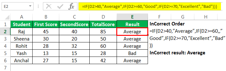
Note: Changing the order of the IF function in Excel would change the result.

Evaluate the formula logic– To see the step-by-step evaluation of multiple IF conditions, we can use the ‘Evaluate Formula’ feature in excel on the “Formula” tab in the “Formula Auditing” group. Clicking the “Evaluate” button will show all the steps in the evaluation process.

For instance, in the second example, the evaluation of the first logical testLogical TestA logical test in Excel results in an analytical output, either true or false. The equals to operator, “=,” is the most commonly used logical test.read more of multiple IF formulas will go as D2>=70; 85>=70; True; Excellent.

Balancing the parentheses: If the parentheses do not match in terms of number and order, then the multiple IF formula would not work.

If we have more than one set of parentheses, the parentheses pairs are shaded in different colors so that the opening parentheses match the closing ones.

Also, on closing the parenthesis, the matching pair is highlighted.

Numbers and Text should be treated differently: The text should always be enclosed in double quotes in the multiple IF formula.

Multiple IF’s can often become troublesome: Managing many true and false conditions and closing brackets in one statement becomes difficult. Therefore, it is always good to use other tools like IF function or VLOOKUP in case Multiple IF’sVLOOKUP In Case Multiple IF’sSometimes while working with data, when we match the data to the reference Vlookup, it finds the first value and does not look for the next value. However, for a second result, to use Vlookup with multiple criteria, we need to use other functions with it.read more are difficult to maintain in Excel.

Recommended Articles

This article is a guide to Multiple IF Conditions in Excel. We discuss using multiple IF conditions, practical examples, and a downloadable Excel template. You may also learn more about Excel from the following articles: –

Источник

Using IF with AND, OR and NOT functions

The IF function allows you to make a logical comparison between a value and what you expect by testing for a condition and returning a result if that condition is True or False.

=IF(Something is True, then do something, otherwise do something else)

But what if you need to test multiple conditions, where let’s say all conditions need to be True or False ( AND), or only one condition needs to be True or False ( OR), or if you want to check if a condition does NOT meet your criteria? All 3 functions can be used on their own, but it’s much more common to see them paired with IF functions.

Use the IF function along with AND, OR and NOT to perform multiple evaluations if conditions are True or False.

IF(AND()) — IF(AND(logical1, [logical2], . ), value_if_true, [value_if_false]))

IF(OR()) — IF(OR(logical1, [logical2], . ), value_if_true, [value_if_false]))

IF(NOT()) — IF(NOT(logical1), value_if_true, [value_if_false]))

The condition you want to test.

The value that you want returned if the result of logical_test is TRUE.

The value that you want returned if the result of logical_test is FALSE.

Here are overviews of how to structure AND, OR and NOT functions individually. When you combine each one of them with an IF statement, they read like this:

AND – =IF(AND(Something is True, Something else is True), Value if True, Value if False)

OR – =IF(OR(Something is True, Something else is True), Value if True, Value if False)

NOT – =IF(NOT(Something is True), Value if True, Value if False)

Examples

Following are examples of some common nested IF(AND()), IF(OR()) and IF(NOT()) statements. The AND and OR functions can support up to 255 individual conditions, but it’s not good practice to use more than a few because complex, nested formulas can get very difficult to build, test and maintain. The NOT function only takes one condition.

Here are the formulas spelled out according to their logic:

=IF(AND(A2>0,B2 0,B4 50),TRUE,FALSE)

IF A6 (25) is NOT greater than 50, then return TRUE, otherwise return FALSE. In this case 25 is not greater than 50, so the formula returns TRUE.

IF A7 (“Blue”) is NOT equal to “Red”, then return TRUE, otherwise return FALSE.

Note that all of the examples have a closing parenthesis after their respective conditions are entered. The remaining True/False arguments are then left as part of the outer IF statement. You can also substitute Text or Numeric values for the TRUE/FALSE values to be returned in the examples.

Here are some examples of using AND, OR and NOT to evaluate dates.

Here are the formulas spelled out according to their logic:

IF A2 is greater than B2, return TRUE, otherwise return FALSE. 03/12/14 is greater than 01/01/14, so the formula returns TRUE.

=IF(AND(A3>B2,A3 B2,A4 B2),TRUE,FALSE)

IF A5 is not greater than B2, then return TRUE, otherwise return FALSE. In this case, A5 is greater than B2, so the formula returns FALSE.

Using AND, OR and NOT with Conditional Formatting

You can also use AND, OR and NOT to set Conditional Formatting criteria with the formula option. When you do this you can omit the IF function and use AND, OR and NOT on their own.

From the Home tab, click Conditional Formatting > New Rule. Next, select the “ Use a formula to determine which cells to format” option, enter your formula and apply the format of your choice.

Edit Rule dialog showing the Formula method» loading=»lazy»>

Using the earlier Dates example, here is what the formulas would be.

If A2 is greater than B2, format the cell, otherwise do nothing.

=AND(A3>B2,A3 B2,A4 B2)

If A5 is NOT greater than B2, format the cell, otherwise do nothing. In this case A5 is greater than B2, so the result will return FALSE. If you were to change the formula to =NOT(B2>A5) it would return TRUE and the cell would be formatted.

Note: A common error is to enter your formula into Conditional Formatting without the equals sign (=). If you do this you’ll see that the Conditional Formatting dialog will add the equals sign and quotes to the formula — =»OR(A4>B2,A4

Need more help?

See also

You can always ask an expert in the Excel Tech Community or get support in the Answers community.

Источник

Источник

The IF function allows you to make a logical comparison between a value and what you expect by testing for a condition and returning a result if True or False.

=IF(Something is True, then do something, otherwise do something else)

So an IF statement can have two results. The first result is if your comparison is True, the second if your comparison is False.

IF statements are incredibly robust, and form the basis of many spreadsheet models, but they are also the root cause of many spreadsheet issues. Ideally, an IF statement should apply to minimal conditions, such as Male/Female, Yes/No/Maybe, to name a few, but sometimes you might need to evaluate more complex scenarios that require nesting* more than 3 IF functions together.

* “Nesting” refers to the practice of joining multiple functions together in one formula.

Use the IF function, one of the logical functions, to return one value if a condition is true and another value if it’s false.

Syntax

IF(logical_test, value_if_true, [value_if_false])

For example:

=IF(A2>B2,»Over Budget»,»OK»)
=IF(A2=B2,B4-A4,»»)

Argument name	Description
logical_test (required)	The condition you want to test.
value_if_true (required)	The value that you want returned if the result of *logical_test* is TRUE.
value_if_false (optional)	The value that you want returned if the result of *logical_test* is FALSE.

Remarks

While Excel will allow you to nest up to 64 different IF functions, it’s not at all advisable to do so. Why?

Multiple IF statements require a great deal of thought to build correctly and make sure that their logic can calculate correctly through each condition all the way to the end. If you don’t nest your formula 100% accurately, then it might work 75% of the time, but return unexpected results 25% of the time. Unfortunately, the odds of you catching the 25% are slim.
Multiple IF statements can become incredibly difficult to maintain, especially when you come back some time later and try to figure out what you, or worse someone else, was trying to do.

If you find yourself with an IF statement that just seems to keep growing with no end in sight, it’s time to put down the mouse and rethink your strategy.

Let’s look at how to properly create a complex nested IF statement using multiple IFs, and when to recognize that it’s time to use another tool in your Excel arsenal.

Examples

Following is an example of a relatively standard nested IF statement to convert student test scores to their letter grade equivalent.

=IF(D2>89,»A»,IF(D2>79,»B»,IF(D2>69,»C»,IF(D2>59,»D»,»F»))))

This complex nested IF statement follows a straightforward logic:

If the Test Score (in cell D2) is greater than 89, then the student gets an A
If the Test Score is greater than 79, then the student gets a B
If the Test Score is greater than 69, then the student gets a C
If the Test Score is greater than 59, then the student gets a D
Otherwise the student gets an F

This particular example is relatively safe because it’s not likely that the correlation between test scores and letter grades will change, so it won’t require much maintenance. But here’s a thought – what if you need to segment the grades between A+, A and A- (and so on)? Now your four condition IF statement needs to be rewritten to have 12 conditions! Here’s what your formula would look like now:

=IF(B2>97,»A+»,IF(B2>93,»A»,IF(B2>89,»A-«,IF(B2>87,»B+»,IF(B2>83,»B»,IF(B2>79,»B-«, IF(B2>77,»C+»,IF(B2>73,»C»,IF(B2>69,»C-«,IF(B2>57,»D+»,IF(B2>53,»D»,IF(B2>49,»D-«,»F»))))))))))))

It’s still functionally accurate and will work as expected, but it takes a long time to write and longer to test to make sure it does what you want. Another glaring issue is that you’ve had to enter the scores and equivalent letter grades by hand. What are the odds that you’ll accidentally have a typo? Now imagine trying to do this 64 times with more complex conditions! Sure, it’s possible, but do you really want to subject yourself to this kind of effort and probable errors that will be really hard to spot?

Tip: Every function in Excel requires an opening and closing parenthesis (). Excel will try to help you figure out what goes where by coloring different parts of your formula when you’re editing it. For instance, if you were to edit the above formula, as you move the cursor past each of the ending parentheses “)”, its corresponding opening parenthesis will turn the same color. This can be especially useful in complex nested formulas when you’re trying to figure out if you have enough matching parentheses.

Additional examples

Following is a very common example of calculating Sales Commission based on levels of Revenue achievement.

=IF(C9>15000,20%,IF(C9>12500,17.5%,IF(C9>10000,15%,IF(C9>7500,12.5%,IF(C9>5000,10%,0)))))

This formula says IF(C9 is Greater Than 15,000 then return 20%, IF(C9 is Greater Than 12,500 then return 17.5%, and so on…

While it’s remarkably similar to the earlier Grades example, this formula is a great example of how difficult it can be to maintain large IF statements – what would you need to do if your organization decided to add new compensation levels and possibly even change the existing dollar or percentage values? You’d have a lot of work on your hands!

Tip: You can insert line breaks in the formula bar to make long formulas easier to read. Just press ALT+ENTER before the text you want to wrap to a new line.

Here is an example of the commission scenario with the logic out of order:

Can you see what’s wrong? Compare the order of the Revenue comparisons to the previous example. Which way is this one going? That’s right, it’s going from bottom up ($5,000 to $15,000), not the other way around. But why should that be such a big deal? It’s a big deal because the formula can’t pass the first evaluation for any value over $5,000. Let’s say you’ve got $12,500 in revenue – the IF statement will return 10% because it is greater than $5,000, and it will stop there. This can be incredibly problematic because in a lot of situations these types of errors go unnoticed until they’ve had a negative impact. So knowing that there are some serious pitfalls with complex nested IF statements, what can you do? In most cases, you can use the VLOOKUP function instead of building a complex formula with the IF function. Using VLOOKUP, you first need to create a reference table:

=VLOOKUP(C2,C5:D17,2,TRUE)

This formula says to look for the value in C2 in the range C5:C17. If the value is found, then return the corresponding value from the same row in column D.

=VLOOKUP(B9,B2:C6,2,TRUE)

Similarly, this formula looks for the value in cell B9 in the range B2:B22. If the value is found, then return the corresponding value from the same row in column C.

Note: Both of these VLOOKUPs use the TRUE argument at the end of the formulas, meaning we want them to look for an approxiate match. In other words, it will match the exact values in the lookup table, as well as any values that fall between them. In this case the lookup tables need to be sorted in Ascending order, from smallest to largest.

VLOOKUP is covered in much more detail here, but this is sure a lot simpler than a 12-level, complex nested IF statement! There are other less obvious benefits as well:

VLOOKUP reference tables are right out in the open and easy to see.
Table values can be easily updated and you never have to touch the formula if your conditions change.
If you don’t want people to see or interfere with your reference table, just put it on another worksheet.

Did you know?

There is now an IFS function that can replace multiple, nested IF statements with a single function. So instead of our initial grades example, which has 4 nested IF functions:

=IF(D2>89,»A»,IF(D2>79,»B»,IF(D2>69,»C»,IF(D2>59,»D»,»F»))))

It can be made much simpler with a single IFS function:

=IFS(D2>89,»A»,D2>79,»B»,D2>69,»C»,D2>59,»D»,TRUE,»F»)

The IFS function is great because you don’t need to worry about all of those IF statements and parentheses.

Need more help?

You can always ask an expert in the Excel Tech Community or get support in the Answers community.

Explanation

This article describes the Excel nested IF construction. Usually, nested IFs are used when you need to test more than one condition and return different results depending on those tests.

Testing more than one condition

If you need to test for more than one condition, then take one of several actions, depending on the result of the tests, one option is to nest multiple IF statements together in one formula. You’ll often hear this referred to as «nested IFs».

The idea of nesting comes from embedding or «nesting» one IF function inside another. In the example shown, we are using nested IF functions to assign grades based on a score. The logic for assigning a grade goes like this:

Score	Grade
0-63	F
64-72	D
73-84	C
85-94	B
95-100	A

To build up a nested IF formula that reflects this logic, we start by testing to see if the score is below 64. If TRUE, we return «F». If FALSE, we move into the next IF function. This time, we test to see if the score is less than 73. If TRUE, we return «D». If FALSE, we move into yet another IF function. And so on.

Eventually, the formula we have in cell D5 looks like this:

=IF(C5<64,"F",IF(C5<73,"D",IF(C5<85,"C",IF(C5<95,"B","A"))))

You can see that it’s important in this case to move in one direction, either low to high, or high to low. This allows us to return a result whenever a test returns TRUE, because we know that the previous tests have returned FALSE.

Making nested IFs easier to read

By their nature, nested IF formulas can be hard to read. If this bothers you, you can add line breaks inside the formula to «line up» the tests and results. This video explains how to add line breaks to a nested if.

Notes

The newer IFS function can handle multiple conditions in a single function.
VLOOKUP can sometimes be used to replace complicated nested ifs.
This article has many more examples of nested ifs.

Источник

This Excel tutorial explains how to nest the Excel IF function with syntax and examples.

Description

The IF function is a built-in function in Excel that is categorized as a Logical Function. It can be used as a worksheet function (WS) in Excel. As a worksheet function, the IF function can be entered as part of a formula in a cell of a worksheet.

It is possible to nest multiple IF functions within one Excel formula. You can nest up to 7 IF functions to create a complex IF THEN ELSE statement.

TIP: If you have Excel 2016, try the new IFS function instead of nesting multiple IF functions.

Syntax

The syntax for the nesting the IF function is:

IF( condition1, value_if_true1, IF( condition2, value_if_true2, value_if_false2 ))

This would be equivalent to the following IF THEN ELSE statement:

IF condition1 THEN
   value_if_true1
ELSEIF condition2 THEN
   value_if_true2
ELSE
   value_if_false2
END IF

Parameters or Arguments

condition: The value that you want to test.
value_if_true: The value that is returned if condition evaluates to TRUE.
value_if_false: The value that is return if condition evaluates to FALSE.

Example (as Worksheet Function)

Let’s look at an example to see how you would use a nested IF and explore how to use the nested IF function as a worksheet function in Microsoft Excel:

Based on the Excel spreadsheet above, the following Nested IF examples would return:

=IF(A1="10x12",120,IF(A1="8x8",64,IF(A1="6x6",36)))
Result: 120

=IF(A2="10x12",120,IF(A2="8x8",64,IF(A2="6x6",36)))
Result: 64

=IF(A3="10x12",120,IF(A3="8x8",64,IF(A3="6x6",36)))
Result: 36

TIP: When nesting multiple IF functions, DO NOT start the second IF function with = sign.

Incorrect formula:
=IF(A1=2,»Hello»,=IF(A1=3,»Goodbye»,0))

Correct formula
=IF(A1=2,»Hello»,IF(A1=3,»Goodbye»,0))

Frequently Asked Questions

Question: In Microsoft Excel, I need to write a formula that works this way:

If (cell A1) is less than 20, then multiply by 1,
If it is greater than or equal to 20 but less than 50, then multiply by 2
If its is greater than or equal to 50 and less than 100, then multiply by 3
And if it is great or equal to than 100, then multiply by 4

Answer: You can write a nested IF statement to handle this. For example:

=IF(A1<20, A1*1, IF(A1<50, A1*2, IF(A1<100, A1*3, A1*4)))

Question:In Excel, I need a formula in cell C5 that does the following:

IF A1+B1 <= 4, return $20
IF A1+B1 > 4 but <= 9, return $35
IF A1+B1 > 9 but <= 14, return $50
IF A1+B1 > 15, return $75

Answer:In cell C5, you can write a nested IF statement that uses the AND function as follows:

=IF((A1+B1)<=4,20,IF(AND((A1+B1)>4,(A1+B1)<=9),35,IF(AND((A1+B1)>9,(A1+B1)<=14),50,75)))

Question: In Microsoft Excel, I need a formula for the following:

IF cell A1= PRADIP then value will be 100
IF cell A1= PRAVIN then value will be 200
IF cell A1= PARTHA then value will be 300
IF cell A1= PAVAN then value will be 400

Answer: You can write an IF statement as follows:

=IF(A1="PRADIP",100,IF(A1="PRAVIN",200,IF(A1="PARTHA",300,IF(A1="PAVAN",400,""))))

Question: In Microsoft Excel, I want to calculate following using an «if» formula:

if A1<100,000 then A1*.1% but minimum 25
and if A1>1,000,000 then A1*.01% but maximum 5000

Answer: You can write a nested IF statement that uses the MAX function and the MIN function as follows:

=IF(A1<100000,MAX(25,A1*0.1%),IF(A1>1000000,MIN(5000,A1*0.01%),""))

Question:I have Excel 2000. If cell A2 is greater than or equal to 0 then add to C1. If cell B2 is greater than or equal to 0 then subtract from C1. If both A2 and B2 are blank then equals C1. Can you help me with the IF function on this one?

Answer: You can write a nested IF statement that uses the AND function and the ISBLANK function as follows:

=IF(AND(ISBLANK(A2)=FALSE,A2>=0),C1+A2, IF(AND(ISBLANK(B2)=FALSE,B2>=0),C1-B2, IF(AND(ISBLANK(A2)=TRUE, ISBLANK(B2)=TRUE),C1,"")))

Question:How would I write this equation in Excel? If D12<=0 then D12*L12, If D12 is > 0 but <=600 then D12*F12, If D12 is >600 then ((600*F12)+((D12-600)*E12))

Answer: You can write a nested IF statement as follows:

=IF(D12<=0,D12*L12,IF(D12>600,((600*F12)+((D12-600)*E12)),D12*F12))

Question:I have read your piece on nested IFs in Excel, but I still cannot work out what is wrong with my formula please could you help? Here is what I have:

=IF(63<=A2<80,1,IF(80<=A2<95,2,IF(A2=>95,3,0)))

Answer: The simplest way to write your nested IF statement based on the logic you describe above is:

=IF(A2>=95,3,IF(A2>=80,2,IF(A2>=63,1,0)))

This formula will do the following:

If A2 >= 95, the formula will return 3 (first IF function)
If A2 < 95 and A2 >= 80, the formula will return 2 (second IF function)
If A2 < 80 and A2 >= 63, the formula will return 1 (third IF function)
If A2 < 63, the formula will return 0

Question:I’m very new to the Excel world, and I’m trying to figure out how to set up the proper formula for an If/then cell.

What I’m trying for is:

If B2’s value is 1 to 5, then multiply E2 by .77
If B2’s value is 6 to 10, then multiply E2 by .735
If B2’s value is 11 to 19, then multiply E2 by .7
If B2’s value is 20 to 29, then multiply E2 by .675
If B2’s value is 30 to 39, then multiply E2 by .65

I’ve tried a few different things thinking I was on the right track based on the IF, and AND function tutorials here, but I can’t seem to get it right.

Answer:To write your IF formula, you need to nest multiple IF functions together in combination with the AND function.

The following formula should work for what you are trying to do:

=IF(AND(B2>=1, B2<=5), E2*0.77, IF(AND(B2>=6, B2<=10), E2*0.735, IF(AND(B2>=11, B2<=19), E2*0.7, IF(AND(B2>=20, B2<=29), E2*0.675, IF(AND(B2>=30, B2<=39), E2*0.65,"")))))

As one final component of your formula, you need to decide what to do when none of the conditions are met. In this example, we have returned «» when the value in B2 does not meet any of the IF conditions above.

Question:I have a nesting OR function problem:

My nonworking formula is:

=IF(C9=1,K9/J7,IF(C9=2,K9/J7,IF(C9=3,K9/L7,IF(C9=4,0,K9/N7))))

In Cell C9, I can have an input of 1, 2, 3, 4 or 0. The problem is on how to write the «or» condition when a «4 or 0» exists in Column C. If the «4 or 0» conditions exists in Column C I want Column K divided by Column N and the answer to be placed in Column M and associated row

Answer:You should be able to use the OR function within your IF function to test for C9=4 OR C9=0 as follows:

=IF(C9=1,K9/J7,IF(C9=2,K9/J7,IF(C9=3,K9/L7,IF(OR(C9=4,C9=0),K9/N7))))

This formula will return K9/N7 if cell C9 is either 4 or 0.

Question:In Excel, I am trying to create a formula that will show the following:

If column B = Ross and column C = 8 then in cell AB of that row I want it to show 2013, If column B = Block and column C = 9 then in cell AB of that row I want it to show 2012.

Answer:You can create your Excel formula using nested IF functions with the AND function.

=IF(AND(B1="Ross",C1=8),2013,IF(AND(B1="Block",C1=9),2012,""))

This formula will return 2013 as a numeric value if B1 is «Ross» and C1 is 8, or 2012 as a numeric value if B1 is «Block» and C1 is 9. Otherwise, it will return blank, as denoted by «».

Question:In Excel, I really have a problem looking for the right formula to express the following:

If B1=0, C1 is equal to A1/2
If B1=1, C1 is equal to A1/2 times 20%
If D1=1, C1 is equal to A1/2-5

I’ve been trying to look for any same expressions in your site. Please help me fix this.

Answer:In cell C1, you can use the following Excel formula with 3 nested IF functions:

=IF(B1=0,A1/2, IF(B1=1,(A1/2)*0.2, IF(D1=1,(A1/2)-5,"")))

Please note that if none of the conditions are met, the Excel formula will return «» as the result.

Question:In Excel, what have I done wrong with this formula?

=IF(OR(ISBLANK(C9),ISBLANK(B9)),"",IF(ISBLANK(C9),D9-TODAY(), "Reactivated"))

I want to make an event that if B9 and C9 is empty, the value would be empty. If only C9 is empty, then the output would be the remaining days left between the two dates, and if the two cells are not empty, the output should be the string ‘Reactivated’.

The problem with this code is that IF(ISBLANK(C9),D9-TODAY() is not working.

Answer:First of all, you might want to replace your OR function with the AND function, so that your Excel IF formula looks like this:

=IF(AND(ISBLANK(C9),ISBLANK(B9)),"",IF(ISBLANK(C9),D9-TODAY(),"Reactivated"))

Next, make sure that you don’t have any abnormal formatting in the cell that contains the results. To be safe, right click on the cell that contains the formula and choose Format Cells from the popup menu. When the Format Cells window appears, select the Number tab. Choose General as the format and click on the OK button.

Question:I’m looking to return an answer from a number ‘n’ that needs to satisfy a certain range criteria. New stamp duty calculators for UK property set bands for percentage stamp duty as follows:

0-125000 =0%
125001-250000 =2%
250001-975000 =5%
975001-1500000 =10%
>1500000 =12%

I realise it’s probably an ‘IF(AND)’ function but I appear to require too many arguments. Can you help?

Answer:You can create this formula using nested IF functions. We will assume that your number ‘n’ resides in cell B1. You can create your formula as follows:

=IF(B1>1500000,B1*0.12, IF(B1>=975001,B1*0.1, IF(B1>=250001,B1*0.05, IF(B1>=125001,B1*0.02,0))))

Since your IF conditions will cover all numbers in the range of 0 to >1500000, it is easiest to work backwards starting with the >1500000 condition. Excel will evaluate each condition and stop when a condition is TRUE. This is why we can simplify the formulas within the nested IF functions, instead of testing ranges using two comparisons such as AND(B1>=125001, B1<=250000).

Question:Let’s expand the last question further and assume that we need to calculate percentages based on tiers (not just on the value as whole):

0-125000 =0%
125001-250000 =2%
250001-975000 =5%
975001-1500000 =10%
>1500000 =12%

Say I enter 1,000,000 in B1. The first 125,000 attracts 0%, the next 125,000 to 250,000 attracts 2%, and so on.

Answer:This adds a level of complexity to our formula since we have to calculate each range of the number using a different percentage.

We can create this solution with the following formula:

=IF(B1<=125000,0, IF(B1<=250000,(B1-125000)*0.02, IF(B1<=975000,(125000*0.02)+((B1-250000)*0.05), IF(B1<=1500000,(125000*0.02)+(725000*0.05)+((B1-975000)*0.1), (125000*0.02)+(725000*0.05)+(525000*0.1)+((B1-1500000)*0.12)))))

If the value was below 125,000, the formula would return 0.

If the value is between 125,001 and 250,000, it would calculate 0% on the first 125,000 and 2% on the remainder.

If the value is between 250,001 and 250,001, it would calculate 0% on the first 125,000, 2% on the next 125,000 and 5% on the remainder.

And so on….

Источник

Multiple IF Conditions in Excel

The multiple IF conditions in Excel are IF statements contained within another IF statement. They are used to test multiple conditions simultaneously and return distinct values. The additional IF statements can be included in the “value if true” and “value if false” arguments of a standard IF formula.

=IF(B1>30,”F”,IF(B1>60,”D”,IF(B1>70,”C”,IF(C5>80,”B”,”A”))))

Multiple IF Condition in Excel
- Explanation
- Examples
  - Example #1
  - Example #2
  - Example #3
  - Example #4
- Things to Remember
- Recommended Articles

Explanation

The IF formula is used when we wish to test a condition and return one value if the condition is met and another value if it is not met.

Each subsequent IF formula is incorporated into the “value_if_false” argument of the previous IF. So, the nested IF excelIn Excel, nested if function means using another logical or conditional function with the if function to test multiple conditions. For example, if there are two conditions to be tested, we can use the logical functions AND or OR depending on the situation, or we can use the other conditional functions to test even more ifs inside a single if.read more formula works as follows:

Syntax

IF (condition1, result1, IF (condition2, result2, IF (condition3, result3,………..)))

Examples

You can download this Multiple Ifs Excel Template here – Multiple Ifs Excel Template

Example #1

Let us say the first score is stored in column B, the second in column C.

The following formula tells Excel to return “Good,” “Average,” or “Bad”:

=IF(D2>=60,”Good”,IF(D2>40,”Average”,”Bad”))

This formula returns the result as given below:

Drag the formula to get results for the rest of the cells.

We can see that one multiple IF function is sufficient in this case as we need to get only 3 results.

Example #2

We want to test one more condition in the above examples: the total score of 70 and above is categorized as “Excellent.”

=IF(D2>=70,”Excellent”,IF(D2>=60,”Good”,IF(D2>40,”Average”,”Bad”)))

This formula returns the result as given below:

Excellent: >=70

Good: Between 60 & 69

Average: Between 41 & 59

Bad: <=40

Drag the formula to get results for the rest of the cells.

We can add several “IF” conditions if required similarly.

Example #3

Suppose we wish to test a few sets of different conditions. In that case, those conditions can be expressed using logical OR and AND, nesting the functions inside IF statements and then nesting the IF statements into each other.

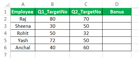
For instance, if we have two columns containing the number of targets made by an employee in 2 quarters: Q1 and Q2. Then, we wish to calculate the performance bonus of the employee based on a higher target number.

We can make a formula with the logic:

If either Q1 or Q2 targets are greater than 70, then the employee gets a 10% bonus,
If either of them is greater than 60, then the employee receives a 7% bonus,
If either of them is greater than 50, then the employee gets a 5% bonus,
If either is greater than 40, then the employee receives a 3% bonus. Else, no bonus.

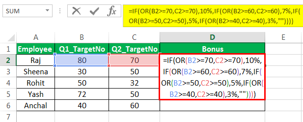
So, we first write a few OR statements like (B2>=70,C2>=70), and then nest them into logical tests of IF functions as follows:

=IF(OR(B2>=70,C2>=70),10%,IF(OR(B2>=60,C2>=60),7%, IF(OR(B2>=50,C2>=50),5%, IF(OR(B2>=40,C2>=40),3%,””))))

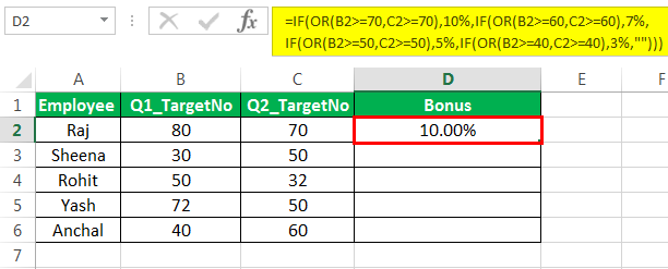
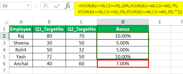
This formula returns the result as given below:

Next, drag the formula to get the results of the rest of the cells.

Example #4

Now, let us say we want to test one more condition in the above example:

If both Q1 and Q2 targets are greater than 70, then the employee gets a 10% bonus
if both of them are greater than 60, then the employee receives a 7% bonus
if both of them are greater than 50, then the employee gets a 5% bonus
if both of them are greater than 40, then the employee receives a 3% bonus
Else, no bonus.

So, we first write a few AND statements like (B2>=70,C2>=70), and then nest them: tests of IF functions as follows:

=IF(AND(B2>=70,C2>=70),10%,IF(AND(B2>=60,C2>=60),7%, IF(AND(B2>=50,C2>=50),5%, IF(AND(B2>=40,C2>=40),3%,””))))

This formula returns the result as given below:

Next, drag the formula to get results for the rest of the cells.

Things to Remember

The multiple IF function evaluates the logical tests in the order they appear in a formula. So, for example, as soon as one condition evaluates to be “True,” the following conditions are not tested.
- For instance, if we consider the second example discussed above, the multiple IF condition in Excel evaluates the first logical test (D2>=70) and returns “Excellent” because the condition is “True” in the below formula:

=IF(D2>=70,”Excellent”,IF(D2>=60,,”Good”,IF(D2>40,”Average”,”Bad”))

Now, if we reverse the order of IF functions in Excel as follows:

=IF(D2>40,”Average”,IF(D2>=60,,”Good”,IF(D2>=70,”Excellent”,”Bad”))

In this case, the formula tests the first condition. Since 85 is greater than or equal to 70, a result of this condition is also “True,” so the formula would return “Average” instead of “Excellent” without testing the following conditions.

Correct Order

Incorrect Order

Note: Changing the order of the IF function in Excel would change the result.

Evaluate the formula logic– To see the step-by-step evaluation of multiple IF conditions, we can use the ‘Evaluate Formula’ feature in excel on the “Formula” tab in the “Formula Auditing” group. Clicking the “Evaluate” button will show all the steps in the evaluation process.
For instance, in the second example, the evaluation of the first logical testA logical test in Excel results in an analytical output, either true or false. The equals to operator, “=,” is the most commonly used logical test.read more of multiple IF formulas will go as D2>=70; 85>=70; True; Excellent.

Balancing the parentheses: If the parentheses do not match in terms of number and order, then the multiple IF formula would not work.
- If we have more than one set of parentheses, the parentheses pairs are shaded in different colors so that the opening parentheses match the closing ones.
- Also, on closing the parenthesis, the matching pair is highlighted.

Numbers and Text should be treated differently: The text should always be enclosed in double quotes in the multiple IF formula.
Multiple IF’s can often become troublesome: Managing many true and false conditions and closing brackets in one statement becomes difficult. Therefore, it is always good to use other tools like IF function or VLOOKUP in case Multiple IF’sSometimes while working with data, when we match the data to the reference Vlookup, it finds the first value and does not look for the next value. However, for a second result, to use Vlookup with multiple criteria, we need to use other functions with it.read more are difficult to maintain in Excel.

General Syntax of Nested IF Statements (Multiple IF Statements)

The general syntax for nested IF statements is as follows:

=IF(Condition1, Value_if_true1, IF(Condition2, Value_if_true2, IF(Condition3, Value_if_true3, Value_if_false)))

This formula tests the first condition; if true, it returns the first value.

If the first condition is false, the formula moves to the second condition and returns the second value if it’s true.

Each subsequent IF function is incorporated into the value_if_false argument of the previous IF function.

This process continues until all conditions have been evaluated, and the formula returns the final value if none of the conditions is true.

The maximum number of nested IF statements allowed in Excel is 64.

Now, look at the following four examples of how to use nested IF statements in Excel.

Example #1: Use Multiple IF Statements to Assign Letter Grades Based on Numeric Scores

Let’s consider the following dataset showing some students’ scores on a Math test.

We want to use nested IF statements to assign student letter grades based on their scores.

We use the following steps:

Select cell C2 and type in the below formula:

=IF(B2>=90,"A",IF(B2>=80,"B",IF(B2>=70,"C",IF(B2>=60,"D","F"))))

multiple if functions to calculate the letter grade of students

Click Enter in the cell to get the result of the formula in the cell.

Copy the formula for the rest of the cells in the column

The assigned letter grades appear in column C.

multiple functions used to calculate the letter grade

Explanation of the formula

=IF(B2>=90,”A”,IF(B2>=80,”B”,IF(B2>=70,”C”,IF(B2>=60,”D”,”F”))))

This formula evaluates the value in cell B2 and assigns an “A” if the value is 90 or greater, a “B” if the value is between 80 and 89, a “C” if the value is between 70 and 79, a “D” if the value is between 60 and 69, and an “F” if the value is less than 60.

Notice that it can be challenging to keep track of which parentheses go with which arguments in nested IF functions.

Therefore, as we enter the formula, Excel uses different colors for the parentheses at each level of the nested IF functions to make it easier to see which parts of the formula belong together.

multiple functions have different color parentheses

Also read: How to use Excel If Statement with Multiple Conditions Range

Example #2: Use Multiple IF Statements to Calculate Commission Based on Sales Volume

Here’s the dataset showing the sales of specific salespeople in a particular month.

data set to calculate commission using multiple if statements

We want to use multiple IF statements to calculate the tiered commission for the salespeople based on their sales volume.

We proceed as follows:

Select cell C2 and enter the following formula:

=IF(B2>=40000, B2*0.14,IF(B2>=20000,B2*0.12,IF(B2>=10000,B2*0.105,IF(B2>0,B2*0.08,0))))

multiple if functions to calculate the commission

Press the Enter key to get the result of the formula.
Double-click or drag the Fill Handle to copy the formula down the column.

The commission for each salesperson is displayed in column D.

commission calculated using multiple IF functions

Explanation of the formula

=IF(B2>=40000, B2*0.14,IF(B2>=20000,B2*0.12,IF(B2>=10000,B2*0.105,IF(B2>0,B2*0.08,0))))

This formula evaluates the value in cell B2 and then does the following:

If the value in cell B2 is greater than or equal to 40,000, the figure is multiplied by 14% (0.14).
If the figure in cell B2 is less than 40,000 but greater than or equal to 20,000, the value is multiplied by 12% (0.12).
If the number in cell B2 is less than 20,000 but greater than or equal to 10,000, the figure is multiplied by 10.5% (0.105).
If the value in cell B2 is less than 10,000 but greater than 0 (zero), the number is multiplied by 8% (0.08).
If the value in cell B2 is 0 (zero), 0 (zero) is returned.

Example #3: Use Multiple IF Statements to Assign Sales Performance Rating Based On Sales Target Achievement

The following is a dataset showing regional sales data of a specific technology company in a particular year.

sales data set where we need to calculate the performance rating

We want to use multiple IF statements to assign a sales performance rating to each region based on their sales target achievement.

We use the following steps:

Select cell C2 and type in the below formula:

=IF(B2>500000, "Excellent", IF(B2>400000, "Good", IF(B2>275000, "Average", "Poor")))

multiple IF functions to calculate the performance rating

Click Enter on the Formula bar.
Drag or double-click the Fill Handle to copy the formula down the column.

The performance ratings of the regions are shown in column C.

Explanation of the formula

=IF(B2>500000, “Excellent”, IF(B2>400000, “Good”, IF(B2>275000, “Average”, “Poor”)))

In this formula, if the sales target in cell B2 is greater than 500,000, the formula returns “Excellent.”

If it’s between 400,000 and 500,000, the formula returns “Good.”

If it’s between 275,000 and 400,000, the formula returns “Average.” And if it’s below 275,000, the formula returns “Poor.”

Example #4: Use Multiple IF Statements in Excel to Check For Errors and Return Error Messages

Suppose we have the following dataset of students’ English test scores. Some scores are less than 0 or greater than 100, and there are no scores in some cases.

data set where some of the scores are missing

We want to use nested IF statements to check for scores in column B and display error messages in column C if there are no scores or the scores are less than 0 or greater than 100.

If the score in column B is valid, we want the formula to return an empty string in column C.

Here are the steps to follow:

Select cell C2 and enter the following formula:

=IF(OR(B2<0,B2>100),"Score out of range",IF(ISBLANK(B2),"Invalid score",""))

nested if function to get the error message

Click Enter on the Formula bar.
Drag the Fill Handle to copy the formula down the column.

The error messages are shown in column C.

Explanation of the formula

=IF(OR(B2<0,B2>100),”Score out of range”,IF(ISBLANK(B2),”Invalid score”,””))

This formula uses the OR function to check if the score in cell B2 is less than 0 or greater than 100, and if it is, it returns the error message “Score out of range.”

The formula also uses the ISBLANK function to check if cell B2 is blank, and if it is, it returns the error message “Invalid score.”

If there is no error, the formula returns an empty string, meaning no message is displayed in column B.

Alternatives to Using Multiple IF Statements in Excel

Formulas using nested IF statements can become difficult to read and manage if we have more than a few conditions to test.

In addition, if we exceed the maximum allowed limit of 64 nested IF statements, we will get an error message.

Fortunately, Excel offers alternative ways to use instead of nested IF functions, especially when we need to test more than a few conditions.

We present the alternative ways in this tutorial.

Alternative #1: Use the IFS Function

The IFS function tests whether one or more conditions are met and returns a value corresponding to the first TRUE condition.

Before the release of the IFS function in 2018 as part of the Excel 365 update, the only way to test multiple conditions and return a corresponding value in Excel was to use nested IF statements.

However, multiple IF statements have the downside of resulting in unwieldy formulas that are difficult to read and maintain.

In some situations, the IFS function is designed to replace the need for multiple IF functions.

The syntax of the IFS function is more straightforward and easier to read than nested IF statements, and it can handle up to 127 conditions.

Here’s an example:

Let’s consider the following dataset showing some students’ scores on a Math test.

data set to calculate the grade of the students

We want to use the IFS function to assign letter grades to the students based on their scores.

We use the following steps:

Select cell C2 and type in the below formula:

=IFS(B2>=90, "A", B2>=80, "B", B2>=70, "C", B2>=60, "D", B2<60, "F")

multiple if functions to calculate the grid of the students

Click Enter on the Formula bar.
Drag or double-click the Fill Handle to copy the formula down the column.

The student’s letter grades are shown in column C.

Explanation of the formula

=IFS(B2>=90, “A”, B2>=80, “B”, B2>=70, “C”, B2>=60, “D”, B2<60, “F”)

This formula tests the score in cell B2 against each condition and returns the corresponding grade letter when the condition is true.

Limitation of IFS Function

The IFS function in Excel is designed to simplify complex nested IF statements.

However, there are situations where the IFS function may not be able to replace nested IF functions completely.

One such situation is when you must calculate or operate based on a condition or set of conditions.

While the IFS function can return a value or text string based on a condition, it cannot perform calculations or operations on that value like nested IF statements.

Another situation where the IFS function may be less useful is when you need to test for a range of conditions rather than just a specific set.

This is because the IFS function requires you to specify each condition and corresponding result separately, which can become cumbersome if you have many conditions to test—in contrast, nested IF statements allow you to test for a range of conditions using logical operators like AND and OR.

The IFS function is a powerful tool for simplifying complex logical tests in Excel.

However, there may be situations where nested IF statements are more appropriate for your needs.

We recommend that you consider both options and choose the one that best fits the specific requirements of your task.

Alternative #2: Use Nested IF Functions

We can use multiple IFS functions in a formula if we have more than one condition to test.

For example, let’s say we have the following dataset of student names and scores on a Physics test in columns A and B.

data set to calculate pass or fail for students

We want to assign a letter grade to each score and include a pass or fail designation based on whether the score is above or below 75.

Here are the steps to use:

Select cell C2 and enter the following formula

=IFS(B2>=90,"A",B2>=80,"B",B2>=70,"C",B2>=60,"D",B2<60,"F")&"  "&IFS(B2>=75,"Pass",B2<75,"Fail")

IFS function to check for multiple conditions

Click Enter on the Formula bar.
Drag or double-click the Fill Handle to copy the formula down the column.

The letter grade and designation of the student scores are displayed in column C.

a result that shows the letter grid and the pass field status

Explanation of the formula

=IFS(B2>=90,”A”,B2>=80,”B”,B2>=70,”C”,B2>=60,”D”,B2<60,”F”)&” “&IFS(B2>=75,”Pass”,B2<75,”Fail”)

This formula uses the first IFS function to assign a letter grade based on the score in column A and the second IFS function to give a pass/fail designation based on the score in column A.

The two IFS functions are combined using the ampersand (&) operator to create a single text string that displays each score’s letter grade and pass/fail designation.

Alternative #3: Use the Combination of CHOOSE and XMATCH Functions

The CHOOSE function selects a value or action from a value list based on an index number.

The XMATCH function locates and returns the relative position of an item in an array. We can combine these functions in a formula instead of nested IF functions.

Here’s an example:

Suppose we have the following dataset showing some students’ scores and letter grades on a Biology test.

data set to calculate the grade point of students

We want to use a formula combining the CHOOSE and XMATCH functions to assign corresponding grade points in column D to each letter grade.

We use the following steps:

Select cell D2 and type in the below formula:

=CHOOSE(XMATCH(C2,{"F","E","D","C","B","A"},0),0,1,2,3,4,5)

choose and match function to calculate grade point

Click Enter on the Formula bar.
Drag or double-click the Fill Handle to copy the formula down the column.

The grade points for each student are displayed in column D.

Explanation of the formula

=CHOOSE(XMATCH(C2,{“F”,”E”,”D”,”C”,”B”,”A”},0),0,1,2,3,4,5)

This formula applies the XMATCH function to find the position of the letter grade in the array {“F”,”E”,”D”,”C”,”B”,”A”}, and then uses the CHOOSE function to return the corresponding grade points.

Alternative #4: Use the VLOOKUP Function

The VLOOKUP function looks for a value in the leftmost column of a table and then returns a value in the same row from a specified column.

We can use the VLOOKUP function instead of nested IF functions in Excel.

The following is an example of using the VLOOKUP function instead of nested IF functions in Excel:

Suppose we have the following dataset showing some students’ scores and letter grades on a Biology test.

We want to use the VLOOKUP function to assign grade points to each student’s letter grade in column D.

We use the steps below:

Create a table that lists the grades and their corresponding grade points in cell range F1:G7.

table that shows the grade based on the grade points

In cell D2, type the following formula:

=VLOOKUP(C2,$F$2:$G$7,2,FALSE)

Note: Use the dollar signs to lock down the cell range F2:G7.

vlookup function to check for multiple conditions

Click Enter on the Formula bar.
Drag or double-click the Fill Handle to copy the formula down the column.

The grade points for each student appear in column D.

result where the grade points are calculated

Explanation of the formula

=VLOOKUP(C2,$F$2:$G$7,2,FALSE)

This formula uses the VLOOKUP function to look up the grade in cell C2 in the table in F2:G7 and return the corresponding grade point in the second column (i.e., column G).

The “FALSE” argument ensures that an exact match is required.

Alternative #5: Use a User-Defined Function

If you need to test more than a few conditions, consider creating a User Defined Function in VBA that can handle many conditions.

Here’s an example of using VBA code to replace nested IF functions in Excel:

Suppose we have the following dataset showing the sales of specific salespeople in a particular month.

We want to use a User Defined Function to calculate the commission for each salesperson based on the following rates:

If the total sales are less than $10,000, the commission rate is 8%.
If the total sales are equal to or greater than $10,000 but less than $20,000, the commission rate is 10.5%.
If the total sales are equal to or greater than $20,000 but less than $40,000, the commission rate is 12%.
If the sales are equal to or greater than $40,000, the commission rate is 14%

We use the following steps:

Open the worksheet containing the sales dataset.
Press Alt + F11 to launch the Visual Basic Editor.
Click Insert on the menu bar and choose Module to insert a new module.

Enter the following VBA code.

'Code developed by Steve Scott from https://spreadsheetplanet.com
Function COMMISSION(Sales As Double) As Double
    Const Rate1 = 0.08
    Const Rate2 = 0.105
    Const Rate3 = 0.12
    Const Rate4 = 0.14

'Calculate sales commissions

    Select Case Sales
        Case 0 To 9999.99: COMMISSION = Sales * Rate1
        Case 10000 To 19999.99: COMMISSION = Sales * Rate2
        Case 20000 To 39999.99: COMMISSION = Sales * Rate3
        Case Is >= 40000: COMMISSION = Sales * Rate4
    End Select

End Function

Save the function procedure and the workbook as a Macro-Enabled Workbook.
Press Alt + F11 to switch to the active worksheet with the sales dataset.
Select cell C2 and enter the following formula:

=COMMISSION(B2)

enter the user defined function in the cell in worksheet

Click Enter on the Formula bar.
Drag or double-click the Fill Handle to copy the formula down the column.

The commission for each salesperson is displayed in column C.

result where the commission is calculated using the UDF

This VBA function takes the sales amount as an argument and returns the corresponding commission.

The User-Defined Function is a much simpler and easier-to-read solution than using nested IF functions.

This tutorial showed four examples of using nested IF statements in Excel and gave five alternatives to using multiple IF statements in Excel. We hope you found the tutorial helpful.

Other Excel tutorials you may find useful:

Excel Logical Test Using Multiple If Statements in Excel [AND/OR]
How to Compare Two Columns in Excel (using VLOOKUP & IF)
Using IF Function with Dates in Excel (Easy Examples)
COUNTIF Greater Than Zero in Excel
BETWEEN Formula in Excel (Using IF Function) – Examples
Count Cells Less than a Value in Excel (COUNTIF Less)

Источник

This is a step-by-step guide on how to use IF function in Excel. It shows you how to create a formula using the IF function, it includes several IF formula examples, an introduction on how to use nested IF formulas, and the exercise file I used when creating this tutorial.

The Excel IF function performs a logical test and returns one value when the condition is TRUE and another when the condition is FALSE.

How do you write an if-then formula in Excel? Well, the syntax for IF statements is the same in all Excel versions. This means that you can use any of the examples shown in this article in Excel for Microsoft 365 or Excel 2021, 2019, 2016, 2013, 2010, 2007, and 2003.

How to use IF function in Excel:

Select the cell where you want to insert the IF formula. Using your mouse or keyboard, navigate to the cell where you want to insert your formula.
Type =IF(
Insert the condition that you want to check, followed by a comma (,). The first argument of the IF function is the logical_test. This is the condition that you want to validate. For example C6 > 70.
Insert the value to display when the condition is TRUE, followed by a comma (,). The second argument of the IF function is value_if_true. Here, you can insert a nested formula or a simple message such as “YES”.
Insert the value to display when the condition is FALSE. The last argument of the IF function is value_if_false. Just like the previous step, you can insert a nested formula or display a message such as “NO”. This can also be set as an empty string (“”), which will display a cell that looks blank.
Type ) to close the function and press ENTER

The following video shows you exactly how to apply the six steps described above and create your first IF formula.

The syntax that shows how to create an IF function in Excel is explained below:
=IF(logical_test, [value_if_true], [value_if_false])

IF is a logical function and implies setting 3 arguments:
logical_test – The logical condition that you want to test. This will return either a TRUE or a FALSE value.
value_if_true – [optional] The value or formula which will be used when logical_test is TRUE.
value_if_false – [optional] The value or formula which will be used when logical_test is FALSE.

Please remember that while both value_if_true and value_if_false are optional, at least one of them needs to be supplied. Otherwise, your IF formula will simply return 0 (zero).

Where is the IF function in Excel? Since this is a logical function, you can find the IF function in the Formulas tab, Function Library section, under Logical.

Logical operators for IF function

The IF function is one of the most used Excel functions, and it allows you to return different values when the logical condition supplied is TRUE or FALSE. An Excel if-then formula can use the following logical operators:

Logical operators	Definition	Example
=	equal to	A1=B1
<>	not equal to	A1<>B1
>	greater than	A1>B1
>=	greater than or equal to	A1>=B1
<	lower than	A1<B1
<=	lower than or equal to	A1<=B1

The IF function doesn’t support wildcards.

Your first IF formula

The IF function runs a logical test and returns different values depending on whether the result is TRUE or FALSE. The result from IF can be a value, a cell reference, or even another formula.

Now let’s move on to some examples.

We’ll be evaluating exam grades. If the student obtained a score higher than or equal to 70, then we will return the message “Pass.” If the grade is lower than 70, then we will display “Fail.”

In this example, I have inserted the following formula in cell F9:
=IF(E9>=70, "Pass", "Fail")

The 3 arguments for this IF formula are:
logical_test: E9>=70
value_if_true: Pass is returned if E9>=70.
value_if_false: Fail is returned if E9<70.

Please note that when you want to use text in your IF formulas (like a word or sentence), you need to wrap the text in quotes (e.g. “Fail”). The only exception is while using TRUE or FALSE, which are built-in functionalities that Excel recognizes automatically.

How to use the IF function in Excel with another function or formula

The beauty of the IF function is that it allows us to build complex financial models with lots of interdependencies. This includes using different formulas based on conditional logic.

In our next example, we will use the IF function to calculate a payment fee based on the value of the order. If the order value is higher than or equal to $1000, then it should calculate a payment fee of 1.00%. However, if the total order value is lower than $1000, then it should use 1.50%.

The formula in cell F31 is:
=IF(E31>=1000, E31*1%, E31*1.5%)

Now let’s look at an IF formula that is dependent on user input. If we select free shipping for the order, then the shipping fee will be set to zero. Otherwise, it will be calculated as 3% of the order value.

This is something really easy to achieve, but it will open up so many opportunities for you to use the IF function in the future.

How to use nested IF statements in Excel

Nesting more IF functions allows you to perform multiple comparisons and create more complex formulas. However, you can only nest up to 64 IF functions in Excel. If you ever reach this limit (I never did), I can guarantee that there is a better and more elegant solution using functions like VLOOKUP, SUMIF, or COUNTIFS.

In the next example, I wrote a formula with several nested IF functions to assign a grade to a list of students based on their test results.

=IF(E71<60, "F", IF(E71<70, "D", IF(E71<80, "C", IF(E71<90, "B", "A"))))

The order of the conditions is important. When the conditions overlap, Excel will retrieve the [value_if_true] argument from the first IF statement that returns TRUE. This is why the conditions from the formula above need to be inserted in the same order for the formula to work properly.

Note: If you are running Office 365, then you can also look at the new IFS function. This function runs multiple tests and returns the value corresponding to the first TRUE result. It’s a very useful alternative to nested IF formulas and makes your formulas much easier to understand by others. You can read more about IFS on Microsoft’s website.

How to use IF formula with OR function in Excel

OR allows you to supply alternative conditions to an IF statement. This opens up opportunities to create complex scenarios where certain behavior is triggered by multiple possible conditions.

Let’s look at an IF formula that calculates a 2.00% shipping fee when the total order value is higher than $1000 or when there are more than 5 items in the order.

The IF OR statement I’ve used in cell H106 is:
=IF(OR(G106>1000, F106>5), G106*2%, 0)

The OR function evaluates if G106>1000 or if F106>5 and the formula returns TRUE when either or both conditions are fulfilled.

How to use IF formula with AND function in Excel

AND allows you to supply multiple criteria to an IF statement. Basically, the IF function returns TRUE if, and only if, all the conditions are met.

Working with our previous example, let’s apply the shipping fee only when the total order value is higher than $1000 and the order contains more than 5 items.

The IF AND statement I’ve used in cell H106 is:
=IF(AND(G128>1000, F128>5), G128*2%, 0)

The AND function evaluates if G106>1000 and if F106>5 and returns TRUE when both conditions are fulfilled.

How to use IF function with VLOOKUP in Excel

VLOOKUP can be nested inside an IF formula to retrieve data when a condition is TRUE or FALSE. In the next example, I will show you how to calculate shipping fees based on a different table that contains the thresholds and percentages to be applied depending on the order value.

The formula I’ve used in cell F152:
=IF(G152="No", VLOOKUP(E152, $J$146:$K$152, 2, TRUE)*E152, 0)

The formula uses the following arguments:
logical_test: G152="No"
value_if_true: VLOOKUP(E152, $J$146:$K$152, 2, TRUE)*E152 is used to retrieve the corresponding shipping fee percentage when G152=”No”
value_if_false: 0 is returned if G152 is anything else than “No.” In our case, the alternative is selecting “Yes” from the drop-down list.

Note: One thing to remember is that I’ve used a VLOOKUP formula with an approximate match argument. This means that your data must be sorted in ascending order by lookup value (in our case, the Order amount).

In case you need additional help, please also read this article that explains step-by-step how to use VLOOKUP function in Excel.

What to do next?

IF is a versatile function that can be used in a wide range of scenarios. I use it daily, and I can’t imagine a world where Excel would lack this functionality.

Practice writing formulas using the IF function, and your spreadsheets will definitely get better and more complex. For example, why not look at another example using an IF function with 3 conditions? It will show you more examples of how to insert an if formula in Excel using nested IF statements and multiple conditions.

Let me know if you have questions on how to use IF function in Excel or if you need advice on how to nest multiple IF statements in your Excel project by leaving a comment below.

Источник

In our last post, we talked about the IF Statement, which is one of the most important functions in Excel. The limitation of the IF statement is that it has only two outcomes. But if you are dealing with multiple conditions then Excel Nested If’s can come in very handy.

Nested if’s are the formulas that are formed by multiple if statements one inside another. This nesting makes it possible for a single formula to take multiple decisions. In Excel 2003 nesting was only possible up to 7 levels but Excel 2007 has increased this number to 64.

Syntax of Excel Nested IF formula:

The syntax of the nested IF statement is as follows:

=IF(Condition_1,Value_if_True_1,IF(Condition_2,Value_if_True_2,Value_if_False_2))

Here, ‘Condition_1’ refers to the condition used in the first IF.
‘Value_if_True_1’ will be the result if the first IF statement is True.
‘Condition_2’ is the condition used in the second IF. The second IF will only come into picture when the First IF statement results a False value.
‘Value_if_True_2’ will be the result if the second IF statement is True.
‘Value_if_False_2’ will be the result if the second IF statement is False.

This is equivalent to:

IF Condition1 = true THEN value_if_true1 'If Condition1 is true
ELSE IF Condition2 = true THEN value_if_true2 'If Condition2 is true
ELSE value_if_false2 'If both conditions are false
END IF 'End of IF Statement

Example of Nested IF’s in Excel:

Now, let’s understand Nested If’s with an example.

Example 1:

In the below image an Employee table of a company is shown. The company decides to give a bonus to its employees but their bonus criteria is quite strange. As you can see in the below image they are giving 20% bonus to the North Region Employees, 30% to the South Region Employees, 40% to the East Region Employees and 50% to the West Region Employees.

In this case, we can use Excel Nested IF formula to find the bonus for each employee. The formula can be:

=IF(B2="North","20%",IF(B2="South","30%",IF(B2="East","40%",IF(B2="West","50%", "Region is Invalid"))))

The formula is quite simple, it just checks if ‘B2’ (the cell that contains region details for the first employee) is equal to “North”, then the value should be 20%, if not then check if B2 is equal to “South”, if yes then the value should be 30%, if not move on to next IF statement and so on.

Similarly, for the second employee the formula would be:

=IF(B3="North","20%",IF(B3="South","30%",IF(B3="East","40%",IF(B3="West","50%", "Region is Invalid"))))

In this case, I have handled another important thing i.e. If the Region does not match with any one of the IF conditions then the output should be “Region is Invalid”.

Example 2:

In the second example, we have a table of students and their scores. Now based on their scores we have to give a grade to the students.

Students with scores below 40 are considered as “Fail”, scores between 41 and 60 are considered “Grade C”, scores between 61 and 75 are considered “Grade B” and scores between 76 and 100 are considered as “Grade A”

In this scenario, we can use a nested If formula as:

=IF(B2<=40,"Fail",IF(AND(B2>=41,B2<=60),"Grade C",IF(AND(B2>=61,B2<=75),"Grade B",IF(AND(B2>=76,B2<=100),"Grade A"))))

This formula just checks if B2 (cell containing the score of the first student) is less than or equal to 40, if true then the value should be “Fail” if not then check the next IF condition and so on.

You can see that here in the inner-most IF statement I haven’t used the ‘Value_if_False’, it is perfectly alright to omit this parameter in such a case. In-case all the IF conditions in this formula will result in a False value then the formula will simply return a ‘FALSE’ keyword.

So, this was all about Nested IF Instruction. Feel free to drop your comments related to the topic.

Источник

Brief syntax lesson

Cells(Row, Column) identifies a cell. Row must be an integer between 1 and the maximum for version of Excel you are using. Column must be a identifier (for example: «A», «IV», «XFD») or a number (for example: 1, 256, 16384)

.Cells(Row, Column) identifies a cell within a sheet identified in a earlier With statement:

With ActiveSheet
  :
  .Cells(Row,Column)
  :
End With

If you omit the dot, Cells(Row,Column) is within the active worksheet. So wsh = ActiveWorkbook wsh.Range is not strictly necessary. However, I always use a With statement so I do not wonder which sheet I meant when I return to my code in six months time. So, I would write:

With ActiveSheet
  :
  .Range.  
  :
End With

Actually, I would not write the above unless I really did want the code to work on the active sheet. What if the user has the wrong sheet active when they started the macro. I would write:

With Sheets("xxxx")
  :
  .Range.  
  :
End With

because my code only works on sheet xxxx.

Cells(Row,Column) identifies a cell. Cells(Row,Column).xxxx identifies a property of the cell. Value is a property. Value is the default property so you can usually omit it and the compiler will know what you mean. But in certain situations the compiler can be confused so the advice to include the .Value is good.

Cells(Row,Column) like "*Miami*" will give True if the cell is «Miami», «South Miami», «Miami, North» or anything similar.

Cells(Row,Column).Value = "Miami" will give True if the cell is exactly equal to «Miami». «MIAMI» for example will give False. If you want to accept MIAMI, use the lower case function:

Lcase(Cells(Row,Column).Value) = "miami"

My suggestions

Your sample code keeps changing as you try different suggestions which I find confusing. You were using Cells(Row,Column) <> "Miami" when I started typing this.

Use

If Cells(i, "A").Value like "*Miami*" And Cells(i, "D").Value like "*Florida*" Then
  Cells(i, "C").Value = "BA"

if you want to accept, for example, «South Miami» and «Miami, North».

Use

If Cells(i, "A").Value = "Miami" And Cells(i, "D").Value like "Florida" Then
  Cells(i, "C").Value = "BA"

if you want to accept, exactly, «Miami» and «Florida».

Use

If Lcase(Cells(i, "A").Value) = "miami" And _
   Lcase(Cells(i, "D").Value) = "florida" Then
  Cells(i, "C").Value = "BA"

if you don’t care about case.

Источник

IF function

Simple IF examples

Common problems

Need more help?

Multiple IFs in Excel

Multiple IF Conditions in Excel

Table of contents

Explanation

Examples

Example #1

Example #2

Example #3

Example #4

Things to Remember

Recommended Articles

Using IF with AND, OR and NOT functions

Examples

Using AND, OR and NOT with Conditional Formatting

Need more help?

See also

Remarks

Examples

Additional examples

Did you know?

Need more help?

Related Topics

Explanation

Testing more than one condition

Making nested IFs easier to read

Notes

Description

Syntax

Parameters or Arguments

Example (as Worksheet Function)

Frequently Asked Questions

Multiple IF Conditions in Excel

Table of contents

Explanation

Examples

Example #1

Example #2

Example #3

Example #4

Things to Remember

Recommended Articles

General Syntax of Nested IF Statements (Multiple IF Statements)

Example #1: Use Multiple IF Statements to Assign Letter Grades Based on Numeric Scores

Explanation of the formula

Example #2: Use Multiple IF Statements to Calculate Commission Based on Sales Volume

Explanation of the formula

Example #3: Use Multiple IF Statements to Assign Sales Performance Rating Based On Sales Target Achievement

Explanation of the formula

Example #4: Use Multiple IF Statements in Excel to Check For Errors and Return Error Messages

Explanation of the formula

Alternatives to Using Multiple IF Statements in Excel

Alternative #1: Use the IFS Function

Explanation of the formula

Limitation of IFS Function

Alternative #2: Use Nested IF Functions

Explanation of the formula

Alternative #3: Use the Combination of CHOOSE and XMATCH Functions

Explanation of the formula

Alternative #4: Use the VLOOKUP Function

Explanation of the formula

Alternative #5: Use a User-Defined Function

Logical operators for IF function

Your first IF formula

How to use the IF function in Excel with another function or formula

How to use nested IF statements in Excel

How to use IF formula with OR function in Excel

How to use IF formula with AND function in Excel

How to use IF function with VLOOKUP in Excel

What to do next?

Syntax of Excel Nested IF formula:

Example of Nested IF’s in Excel: