
Содержание
- How to Create a Google Map From Excel
- Related
- Launching Google Maps from Excel with Chrome browser
- Effective geocoding in Python free of charge
- Folium Draw plugin – extended functionality
- Styling on-click marker on Python Folium map
How to Create a Google Map From Excel

Google maps plot locations based on latitude and longitude coordinates. When Microsoft Excel sends these coordinates to Internet Explorer, Google Maps can use them to create new maps relevant to your workbook. For example, if you create spreadsheets for transactions at different branches of your company, you can type each branch’s coordinates into the specific cells on the sheet to pinpoint their locations on a Google map.
Open Excel and then press «Alt-F11» to open Excel’s Visual Basic editor. Double-click «Module 1» in the project window to open a blank module window. (If Module 1 is not visible, select «Insert Module» from the Insert menu.)
Copy and paste the following into the new window to create a routine for opening a browser window:
Sub OpenURL(urlName) Dim browserWindow As Object Set browserWindow = CreateObject(«InternetExplorer.Application») ie.navigate urlName End Sub
Copy and paste the following after the previous routine to create a routine for generating a Google Maps URL:
Sub mcrURL() Dim url As String url = «https://maps.google.com/?ll=» & Range(«A3»).Value & «,» & Range(«A4») Call OpenURL(url) End Sub
Replace «A3» and «A4» in the previous routine with the addresses for the cells where you plan to insert the location’s coordinates.
Return to your spreadsheet and click «Insert» in the Developer ribbon. (See Tips to display the Developer ribbon if it is not yet displayed.)
Click a button icon and then click and drag over the spreadsheet to create a button and open the Assign Macro dialog box.
Type «mcrURL» into the «Macro name» text box if it is not already there and click «OK.»
Type a latitude into the first cell that you selected in Step 4 and type a longitude into the second cell. For example, type «40.71» into cell A3 and «-74.006» into cell A4
Click the button that you added to open the Google map.
Источник
Launching Google Maps from Excel with Chrome browser

Pic. 10 The example of getting multiple directions with Google Maps and VBA Excel.

Effective geocoding in Python free of charge

Folium Draw plugin – extended functionality

Styling on-click marker on Python Folium map
The work with addresses is quite often in our Excel spreadsheet. Today I would like to demonstrate to you how to parse the address string in the Excel cell in order to make it auto-populated on Google Maps or any other website. Nowadays many websites feature the permalink , which makes them more dynamic. The permalink is helpful in reaching the specific item on the websites. Because we are going to deal with the address the most important websites are map-based. The permalink in this kind of website can be based on address or coordinates. If we take into account Google Maps, our today’s example, we can see how the permalink works(Pic. 1).

Pic. 1 Google Maps permalink elements: 1 – main address; 2 – coordinates; 3 – zoom factor (Google Maps & Terrain) or height above the ground (google satellite); 4 – a place populated by postcode; 5 – full address; 6 – directions; 7 – direction between places (from/to); 8 – search nearby; 9 – object type search. All of them are distinguished by specified colors in order to better understand.
As you can see, Google Maps have a dynamic permalink , depending on the operations, which can be done. This example roughly shows the importance of the permalink, which makes the website dynamic, as mentioned above. This situation applies to the other websites too.
Knowing how Google Maps permalink works, now we can devise some way how to grip it from MS Excel.
First of all, we can divide this URL string between the generic part and the dynamic part . The generic part is definitely the “http://google.com/maps/“, marked as the main web address (Pic. 1) which won’t change at all. The second part if behind the slash and it will change as we do some operations on the website.
So the second part of this link can be reliant on the string, which we prepared in our MS Excel document . This string is obviously the address, but it must be formatted correctly if we wish to use it along with the Google Maps permalink.
Before I show you how to parse the Excel address string let’s see how Google Chrome works with VBA Excel.
The most simple way to open any website in Google Chrome using VBA Excel is like in the code below or here.
Sub Chromeweb()
Dim chromePath As String
chromePath = “””C:ProgramFiles(x86)GoogleChromeApplicationChrome.exe”””
Shell (chromePath & ” -url http:maps.google.com”)
End Sub
Launching this macro we can open the Google.com website. However, there are 2 basic things to mention, before you copy & paste this code. The first one is the destination folder path for our Chrome application in Windows , which is mostly the same, although if you did the custom installation it is good to check it. The second one is the target website , which can be any other than Google (behind the -url just swap the maps.google.com link with yours).

Pic. 2 Default view of Google Maps launched by VBA Excel macro for Google Chrome.
The basic macro for launching a Google Chrome address is not enough to make the full permalink management in Google Maps, what we need now. This code is not able to manage the dynamic website.
To make our VBA Excel macro more flexible regarding dynamic websites, we must expand it.
The most reasonable way to launch various website permalinks in Chrome is using the Selenium software .
Selenium is one of the web test tools, which gives you much more functionality within the objects, that you can control. These objects are i.e. websites, from where you can easily scrap the interesting content or simply automate them. In our case, the second attitude is very important because we want to have our Google Maps permalink being flexible.
There are quite a few sources, where the appliance Selenium with the VBA Excel code has been explained in detail. There are a few steps to do so. However, for parsing the Excel address in Google Maps or other small stuff on different websites we don’t really need the Selenium setup. This is the major goal of this article, to show you how can you make the Google Maps platform dynamic on the basis of the VBA Excel macro only . You will spend a bit less time doing this, getting pretty much the same effect.
Before we will get started it’s important to check the Google Maps permalink again. As you can see above (Pic. 1), the permalink includes some strings linked by “+” or eventually the coma (not to mention the slashes typical for any web address).
Now, we must prepare our address string in Excel in order to match it with the Google Maps permalink. Let me show some steps on how to do this with a single address.
Your example address in excel is:
4, Howburn Court, Aberdeen, AB11 6YA
based in cell A1.
So you have effectively two options to show it in Google Maps. There is a third option available also, but I am leaving the geocoding issue for the next time.
The first option is extracting the postcode only and incorporating it into the Google Maps permalink. The second way is to parse our whole address . By the looks of it, our example address in Excel has some fixed spaces , which usually occur. These fixed spaces you can see as commas or simply the spaces between the words.
In order to adjust our address string to the Google Maps permalink, we must do some necessary alterations to this string.
If we are going to extract the postcode only , the useful option will be extraction the last characters from the string . The number of characters will depend on our postcode description. In the UK the postcode comprises 2 single characters (AB11 6YA) separated by space, so we must extract 2 last characters from our string. In Poland for example the postcode contains one character (38-400), so only the last character extraction will be required.
Staying with our example, we must extract the last two characters then. For this purpose we need formulas like this:
=TRIM(RIGHT(SUBSTITUTE(A1,” “,REPT(” “,60)),120))
=MID(A1,FIND(“@”,SUBSTITUTE(D18,” “,”@”,LEN(A1)-LEN(SUBSTITUTE(A1,” “,””))-1))+1,100)
which extracts the full UK postcode for us. When you replace my cell with yours, the result you are getting should be the postcode only for this location:
AB11 6YA
In this event, the last step left. As you have noticed in the Google Maps permalink this is a “+” symbol, connecting the characters. There is an easy function in Excel, which can swap our space quickly with the “+” symbol. This is the SUBSTITUTE function.
Seeing this formula above, it’s easy to understand what is happening. We are filling up space with the “+” figure. Now our postcode string has been turned into one character.
AB11+6YA
Now our postcode in cell A3 should be ready to populate in Google Maps permalink. It would work, but there is some mismatch in this method, which causes a lack of response from the permalink. As a result, our default location is opened. I would suggest doing an additional parse of this postcode . First of all, we need to extract one element from our postcode. It must be the major part of our postcode – AB11. In this event we must use the following formula:
= LEFT(A2,FIND(” “,A2) -1)
As you may have noticed I am doing this operation on my original postcode, including space between two characters. The -1 means, that I must remove the space between AB11 and 6YA.
As a result, I should get:
AB11
Now, the very last step is to concatenate our piece of a postcode (cell A3) with the substituted one in cell A4, which includes the “+” symbol. It can be done quickly with the CONCATENATE function.
=CONCATENATE(A3,”+”,A4)
We must input the “+” between these 2 cells, as we still need our string in one piece. Finally, we are getting, the postcode string in cell A5 as per below:
AB11+6YA+AB11
which is ready to be parsed in the Google Maps permalink.
That’s all with the pure Excel stuff. Now, we must use the proper VBA code to create the working macro.
I showed you above the very basic macro solution for launching the webpage straight from Excel. Now we must expand it, enabling us to take advantage of the dynamic webpage.
First of all, the two-part VBA code needed, which includes the function.
Sub GoogleMapsChrome()
Dim Postcode As String
Dim url As String
Postcode = Sheets(“Sheet1”).Range(“A5”).Value
url = “https://www.google.com/maps/place/+” & Postcode
OpenChrome url
End Sub
Sub OpenChrome(url As String)
Dim Chrome As String
Chrome = “C:Program Files (x86)GoogleChromeApplicationChrome.exe -url”
Shell (Chrome & ” ” & url)
End Sub
Now, let me explain the code above:
Firstly we need to declare our variables, which are the postcode and the web link.
Our postcode is based in cell A5 including our final address string in Excel, which is now: AB11+6YA+AB11.
Our target URL path is Google Maps permalink, which is to be based on our address. If the Google Maps permalink comprises basically 2 elements: a generic and dynamic one, we will determine the string of its second element.
As it was shown above (Pic. 1), the generic part of the Google Maps address is http://Google.com/maps. The dynamic starts from the 2 nd piece, which varies accordingly as our purpose of use changes. If we want to find the address-based place, then the generic part of the permalink will be http://www.google.com/maps/place/.
Next, everything beyond this slash is expressed by a “+” figure, appearing everywhere, where would be simply space. Although the “+” symbol doesn’t appear straight after the slash nowhere in the address (Pic. 1), it remains necessary for further autoredirection done by Google Maps. Regarding this situation, we can add up the first “+” symbol straight beyond the last slash, making our fixed part of the link ready to use with the parsed Excel variable. Our link will look as follows: http://www.google.com/maps/place/+ .
What is happening next? We are chaining this link with our prepared address string in cell A5, which has been declared as a variable with the Dim statement.
The last line of code represents the function needed to open this link in Google Chrome. The function written underneath includes the basic command for launching the Chrome browser, as discussed previously.

Pic. 3 The Excel file with the address string parsing for Google Maps permalink purposes. The button with macro has been already added.
Above you can spot all the cells used for the purpose of this brief tutorial. The code shown above has been assigned to the button . Now once you click this button, Chrome should open Google Maps under the given address (Pic. 4). Wait maybe 2-3 seconds and see how the platform deals with the redirection. Now the “+” symbol behind the slash is gone and new permalink elements become visible (Pic. 5).

Pic. 4 Our postcode has been used as the part of Google Maps permalink. In the effect, the website is opening under the given address.

Pic. 5 The permalink with Excel Address being redirected to the proper Google Maps Permalink including the information about the highlighted place.
This is a simple method to open Google Maps under our desired address. We used only the postcode. It will be valid for finding the place itself, although if you want to search nearby this place it’s better to parse a whole address.
For this purpose, we must do one basic step, which will change the comma & space with the “+” symbol for us.
The quickest way to write it down is the double SUBSTITUTE function. Let’s put our cell A7 in this formula and see what happens.
=SUBSTITUTE(SUBSTITUTE(A1,”,”,””),” “,”+”)
We are replacing the comma with the vacuum, without space, which is marked as the “” symbol (nothing in the quotes), and the existing space with the “+” symbol at the same time. The existing space is always marked as “something” between the quotes: ” “.
As a result, we are getting a whole address string parsed for Google Maps purposes.
4+Howburn+Ct+Aberdeen+AB11+6YA
If we supersede this address string with the postcode shown previously, Google Maps should be opened under the same address, but in this case, the platform is more precise (Pic. 6).

Pic. 6 The specified location opened in Google Maps as the effect of parsing the full address string in MS Excel.
Now it looks like we gained instant access to the Street View, which wasn’t so easily reachable previously (Pic. 5), apart from the yellow pegman, which is always present.
Like I said before, Google Maps it’s not only an address finder. We can also search for places near our location.
In this situation, small changes in our VBA code are required. We must change the Google Maps link, equipping it with the type of place, which we are looking for.
Sub GoogleNearby()
Dim Postcode As String
Dim urlB As String
Postcode = Sheets(“Sheet1”).Range(“A7”).Value
urlB = “https://www.google.com/maps/search/mcdonalds+near+” & Postcode
OpenChrome urlB
End Sub
Treat it code as another macro. We are using the OpenChrome function again. See, what had changed here. The Google maps permalink as the urlB variable now includes the “search” section with the Mcdonald’s parsed with the “+” symbol. After this string, we can input our address defined in cell A7 by the existing VBA code.
The result will be nice. All the Mcdonald’s will be populated near our defined place (Pic. 7).

Pic. 7 Mcdonald’s nearest to our address populated by the “Search nearby” option in Google Maps straight from Excel.
The last thing to discuss in this article is the management of the direction . As we can easily open Google Maps under our address, we can get the relevant directions too. There are effectively 2 options to do so. The first option comes from the generic link leading to our current location, which is described below:
https://www.google.com/maps/dir/my+location/
and the second option, which requires adding a separate address, from where we want to get directions to our current location.
The first option requires only one address, which we are dealing with. Another one comes from our location. I am assuming, that you don’t need more addresses than 2. We will discuss later how to use a multitude of addresses in our direction.
In this simplest event our VBA code will look as follows:
Sub Directions()
Dim location As String
Dim urlC As String
location = ThisWorkbook.Sheets(“Sheet1”).Range(“A7”)
urlC = “https://www.google.com/maps/dir/my+location/” & location
OpenChrome urlC
End Sub
Obviously, your OpenChrome function has been set earlier.
As a result, you should have Google Maps opened with your directions. Take a look at how the permalink changes, where /my+location/ is superseded by the closest address corresponding to the current location of our device (Pic. 8).

Pic. 8 The example of getting directions with Google Maps and VBA Excel. The upper image shows the initial permalink, as comes from our code. The lower image shows the permalink after Google Maps correction with the current address of our device, where: 1 – the generic part of Google Maps permalink; 2 – the address of our current location.
In the case of the second option considered, we must add another address, independent of our location . Imagine, that your new address is based on column A9 from now. This is a new variable, which we must define in our VBA code in order to make it run.
Let’s add this new variable to our existing code, which should look like this:
Sub Directions()
Dim location As String, location2 As String
Dim urlC As String, urlD As String
location = ThisWorkbook.Sheets(“Sheet1”).Range(“A7”)
location2 = ThisWorkbook.Sheets(“Sheet1”).Range(“A9”)
urlC = “https://www.google.com/maps/dir/my+location/” & location
urlD = “https://www.google.com/maps/dir/” & location & “/” & location2
OpenChrome urlC
OpenChrome urlD
End Sub
, where these 2 methods have been included.
Considering our new line of code, we must be aware of the order of our addresses . The first address is always our starting point, and the second one is our destination. It’s easy to mix (Pic. 9).

Pic. 9 The example of getting directions with Google Maps and VBA Excel. Look at the address order: 1 – the starting location; 2 – the target location.
The last exercise to work with is adding multiple addresses to our permalink. Everyone knows, that Google enables us to input at least several addresses on our way between the start and finish of our journey. It can be done, by clicking the “+ Add destination” option. To give it a ride via the VBA code, we need at least one other address. We can add the new address to our cell A10 for instance.
Next, following the previous procedure, we need another variable defined in our code, which should look as follows:
Sub Directions()
Dim location As String, location2 As String, location3 As String
Dim urlE As String
location = ThisWorkbook.Sheets(“Sheet1”).Range(“A7”)
location2 = ThisWorkbook.Sheets(“Sheet1”).Range(“A9”)
location3 = ThisWorkbook.Sheets(“Sheet1”).Range(“A10”)
urlE = “https://www.google.com/maps/dir/” & location & “/” & location2 & “/” & location3
OpenChrome urlE
End Sub
, including only one URL this time.
In turn, our route has been expanded to this new address (Pic. 10).

Pic. 10 The example of getting multiple directions with Google Maps and VBA Excel.
Now we have got three addresses populated in Google Maps, which show our entire route.
So we are done for now. Our final excel document should look like below (Pic. 11) and it’s downloadable here. If you wish to go through this whole task again and get more practice, you can use this file.

Pic. 11 The screenshot of my Excel file tailored for opening addresses in Google Maps.
Launching Google Maps from Excel I just wanted to show you the deal of VBA Excel macros with the websites and their permalinks .
Google Maps is only one example of using it. You can use this advice for other websites & map servers, depending on their permalinks. The issue will be similar. Make sure, that you are confident of the permalink of that given website before you start preparing variables in the spreadsheet and coding macros. Make sure, that there are no frill spaces, commas, etc. You should also double-check the order, in which all the permalink pieces are located. If everything is alright, then you definitely will be successful. Google Chrome browser doesn’t really need the Selenium software if all our elements are deliberately prepared at the Excel spreadsheet stage. Good luck!
Links:
Forums:
My questions:
Wiki:
Youtube:
Источник
This article will explain how to build a custom URL to open Google Maps or Bing Maps with addresses in your cells.
Google Maps or Bing Maps
Both map services offer the ability to build custom URLs but, there are differences. For example,
- Bing Maps does not allow building a URL from a postal address
- Satellite maps are only possible with latitude and longitude (not with postal addresses)
The LINK_HYPERTEXT function
To build a custom URL in Excel, all you have to do is write this URL, as a character string, in the HYPERLINK function.
=HYPERLINK(«https://www.google.com/maps»)

You can customize your URL by filling in the function’s second argument.
=HYPERLINK(«https://www.google.com/maps»; «Google Map»)

Build a Custom Google Maps URL
We will take these addresses as an example.

Now, to build the custom Google maps URL, we must start with this link
https://www.google.com/maps/search/?api=1&query=
Then, we add the addresses in our cells, with the & symbol. We can use either the reference of a cell or the reference of a Table.
=HYPERLINK(«https://www.google.com/maps/search/?api=1&query=»&[@ Address]; «Google Maps»)
When you click on the link, you immediately open Google Maps, with the correct location, in your browser😉👍

URL with latitude and longitude
Nowadays, collecting GPS coordinates becomes easier with mobile devices. And, you can convert your addresses to GPS coordinates using a Google API.
To check each GPS coordination, you can also create your custom Google Maps link (file here)
The Google URL is different from the previous URL with a search by postal address. The separator between latitude and longitude is the comma.
https://www.google.com/maps/@?api=1&map_action=map¢er=
When applied to the HYPERLINK formula, it gives
=HYPERLINK(«https://www.google.com/maps/@?api=1&map_action=map&center=» &A2&»,»& B2)
CAUTION! the point is the only decimal separator allowed for the latitude and longitude (not the comma)

The Bing Maps writing is shorter. The separator between latitude and longitude is the tilde «~»
https://bing.com/maps/default.aspx?cp=latitude~longitude
And in a formula it gives
=HYPERLINK(«https://bing.com/maps/default.aspx?cp=»&A2&»~»&B2)
Show Satellite Map
To display the result as a Satellite view, you can only use latitude and longitude. The option isn’t available with postal addresses.
With Google, you must add the parameter basemap=satellite
https://www.google.com/maps/@?api=1&map_action=map&center=latitude,longiture&basemap=satellite
=HYPERLINK(«https://www.google.com/maps/@?api=1&map_action=map&center=»&A2&»,» &B2& «&basemap=satellite»)

With Bing, you must add the parameter &style=h (display the indications on the map) or &style=a (display only the image)
And the formula is
=HYPERLINK(«https://bing.com/maps/default.aspx?cp=»&A2&»~» &B2&»&style=h»)
Adjust the zoom in your URL
You can also specify the zoom level with Google and Bing, always from a latitude and longitude.
With Google, you just have to add the parameter &zoom with a value between 0 and 21 (default 15). The closer to 21, the closer the zoom.
=HYPERLINK(«https://www.google.com/maps/@?api=1&map_action=map&center=»&A2&»,»&B2& «&basemap=satellite&zoom=20»)

With Bing, the zoom level is expressed with the &lvl parameter and a value between 1 and 20. The closer to 20, the closer the zoom.
=HYPERLINK(«https://bing.com/maps/default.aspx?cp= &A2&»~»&B2&»&style=h&lvl=19»)
Содержание
Это моя первая попытка использовать карты Google в Excel (скачать ниже). В настоящее время я могу ввести адрес и получить карту Google адреса, отображаемую в Excel, с большинством интересных функций Google.
Несколько эскизов таблицы Excel Google Map, щелкните, чтобы просмотреть увеличенные изображения.
Нормальный вид
 Увеличенный гибридный вид

Таблица Google Map использует для работы два API: Geocoder.us Api и Google Maps Api. Я подумывал также добавить текущий прогноз погоды, но пока воздержался.
Итак, как это работает?
Резюме:
1. Адрес отправляется на Geocoder.us для преобразования в широту и долготу (необходимые для отображения местоположения на картах Google), а результат возвращается в электронную таблицу.
2. Excel отправляет эту геокодированную информацию на сервер easyexcel.net, где у меня есть карта Google, которая принимает широту и долготу в качестве переменных и отображает соответствующую карту через API карт Google.
3. Наконец, в Excel есть элемент управления веб-браузера, который переходит на этот новый адрес.
Немного больше:
1. Чтобы поэкспериментировать с отправкой адреса и заставить Geocoder.us возвращать широту и долготу обратно в Excel, я создал книгу геокодирования для экспериментов.
2. Щелкните эту ссылку, чтобы увидеть мою веб-страницу, которая получает широту и долготу в качестве переменных и возвращает соответствующую карту (посмотрите в адресной строке). Если вы хотите создать похожую страницу, вы можете просмотреть код моей страницы здесь: googlemap.txt. (Да, это взломано вместе. Не забудьте ввести свой собственный ключ API Google в разделе Head.)
3. Я установил margin: 0px, чтобы убрать пробелы вокруг карты, пытаясь сделать его менее похожим на элемент управления веб-браузера и больше на элемент управления Google.
Требования
Чтобы использовать электронную таблицу, вам понадобится Excel 2003. Я тестировал его на этом. Я считаю, что для Excel 2002 «импорт кода vba» немного отличается, и потребуется небольшая настройка.
Чтобы создать собственное решение, вам понадобится ключ разработчика Google, веб-сайт для размещения страницы и Excel 2003.

Щелкните эту ссылку, чтобы загрузить карту Google в виде таблицы Excel.
Обновлять:
Канадские карты Google Maps в Excel, которые работают с версиями Excel до 2003 года.
Случайный:
-Вы можете делать гораздо больше с картами Google, чем просто наносить точки, мне особенно нравится этот пример: gMap Workout Tracker
-Microsoft представила свой новый картографический сервис на этой неделе: Virtual Earth (открывается в новом окне, так как у них отключена кнопка возврата). Спутниковые снимки в моем районе намного лучше, чем карты Google, и в интерфейсе есть несколько дополнительных интересных трюков. Я еще не пробовал API виртуальной земли. Дьюла Гуляс взял мои оригинальные Карты Google в Excel и внес в них два изменения, которые могут заинтересовать некоторых читателей:
1. Он предоставляет интерфейс для США и Канады.
2. Он использует Microsoft XML, V3.0, поэтому работает с парой версий Excel до 2003 года.
Канадский GoogleMap Excel 2000
Очень круто! Дьюла использовал Geocoder.ca для кодирования канадских адресов.
Вы можете отправлять любые «комментарии / улучшения кода / предложения» напрямую по адресу: gygulyas -at- yahoo.ca
Я побывал в нескольких местах Онтарио и мне всегда нравится Канада.
Пару лет назад, уезжая из Торонто, я оказался в северной части штата Нью-Йорк, а не в Кентукки, совсем недалеко (нет, я был не единственным в машине, так что я уверен, что смогу использовать канадскую версию.
Вы поможете развитию сайта, поделившись страницей с друзьями
Here’s my first attempt at using Google maps in excel (download below). Currently I can input an address and have a Google map of the address displayed in Excel, with most of the cool google functionality.
A couple thumbnails of the Excel Google Map Spreadsheet, click to view the larger images.
Normal View

Zoomed Hybrid View

The Google Map Spreadsheet uses two API’s to work, the Geocoder.us Api and Google Maps Api. I thought about also throwing in the current weather report, but refrained for now.
So how does it work?
Summary:
1. The address is sent to Geocoder.us to be converted to Latitude and Longitude (required to map a location on google maps), and the result is returned to the spreadsheet.
2. Excel sends this geocoded information to the automateexcel.com server, where I have a google map that receives latitude and longitude as variables and displays the respective map via the Google Map API.
3. Finally there’s a web browser control in Excel that navigates to this new address.
A bit more:
1. To experiment with sending an address and having Geocoder.us return the Latitude and Longitude back to Excel, I created a Geocoding workbook to experiment with.
2. Click this link to see my webpage that receives latitude and longitude as variables and returns the respective map (look in the address bar). If you’d like to create a similar page you can view my page code here: googlemap.txt. (Yep, it’s hacked together. Remember to input your own Google API Key in the Head section.)
3.I set margin:0px to remove the whitespace around the map, trying to make it look less like a web browser control and more like a google control.
Requirements
To use the spreadsheet you’ll need Excel 2003. That’s what I’ve tested it on, for Excel 2002 I believe the “import vba code” is slightly different and minor tweaking will be needed.
To create your own solution you’ll need a Google Developer Key, a Website to host the page, and Excel 2003.

Click this link to download the Google Map in Excel Spreadsheet
Update:
A Canadian Google Maps In Excel that works with pre-2003 Excel versions.
Random:
-You can do much more with google maps than just plotting points, I particularly like this example: gMap Workout Tracker
-Microsoft unveiled their new mapping service this week: Virtual Earth (Opens in new window since they have the back button disabled). The satellite imagery in my neighborhood is much nicer than google maps, and the interface has some additional cool tricks. I haven’t tried the virtual earth api yet.
 Gyula Gulyas took my original Google Maps in Excel and made two changes to it that some readers may be interested in:
1. It provides a US and Canada interface
2. It uses Microsoft XML, V3.0, so it works with a couple versions of Excel prior to 2003
Canadian GoogleMap Excel 2000
Very cool! Gyula made use of Geocoder.ca for the goecoding of Canadian addresses.
You can send any “comments/code improvements/ suggestions” directly to: gygulyas -at- yahoo.ca
I’ve been to a few spots in Ontario and always enjoy Canada.
A couple years ago leaving Toronto I ended up in upstate New York instead of Kentucky, just a bit off (no I wasn’t the only one in the car 🙂 so I’m sure I can use the Canadian version.
Суть сабжа в ледующем. Есть гугл таблица с адресами и есть гугл карта. Все известно, что можно атвоматом выгрузить адреса на карту с таблицы, очень удобно и круто. Как сделать так, чтобы при автоматическом изменении данных в таблицах — менялись данные на карте(добавились новые адреса или удалились старые)? Сейчас получается нужно каждый раз перезагружать таблицу, удалять и подгружать документы вновь.
Всем спасибо, нужно прямо рабочий вариант, тема для меня очень актуальна.
-
Вопрос заданболее трёх лет назад
-
2049 просмотров
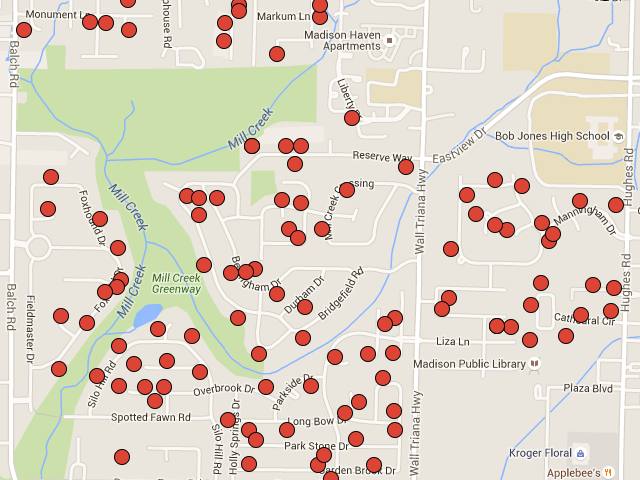
An address map is a valuable way of representing points of data. We’ve been asked to create membership maps for organizations. A request by a church to make a map showing church member addresses inspired us to write up this method of making an address map.
Google Map’s Your Places is an easy and free portal to seeing your spreadsheet data in an online map. While there are more involved ways of accomplishing this, including linking an online version of your spreadsheet data “live” to Google Maps, let’s explore the simplest way of mapping your Excel data.
(Note that some of the menus and names of interface features change when Google decides to update this service.)
GOOGLE ACCOUNT & MICROSOFT EXCEL
To start, you’ll need a Google account. You can create one at Google. For a user name either create a Gmail address or just use an existing, non-Google email address.
The other pre-requisite you’ll need is a Microsoft Excel spreadsheet with location data. For this blog post, I employed a spreadsheet of parishioners provided by a church office that has columns for name, street address, city, state, and zipcode.
GOOGLE’S YOUR PLACES
Once your account is set up and your spreadsheet populated with data, you’re ready to begin. Go to Google Maps and click the three-line “hamburger menu” icon in the upper-left.
![]()
This opens the Google Maps menu with different options. You’re interested in Your Places.
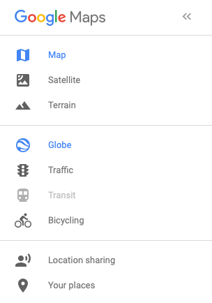
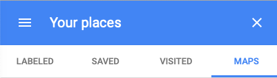
Now click Your Places mid-way down the menu.
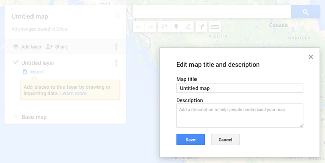
CREATE YOUR MAP
Next, click CREATE MAP at the bottom of the menu. This brings up the new map box in which you’ll edit information about the map and import data into one of its layers.In the new map box, click on Untitled map and give the map a suitable name in the pop-up Edit map title and description box.

Next, click on “Import” in the new map box and then in the pop-up import box, drag and drop the icon of your spreadsheet. This initiates Google’s processing of your data.
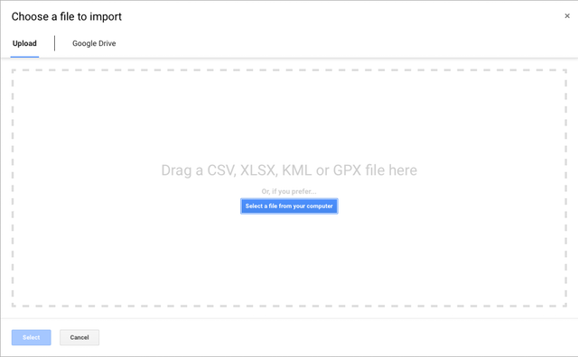
Drag your Excel file, or other file type, to the import box.
CONNECTING EXCEL COLUMNS TO GOOGLE PLACEMARKS
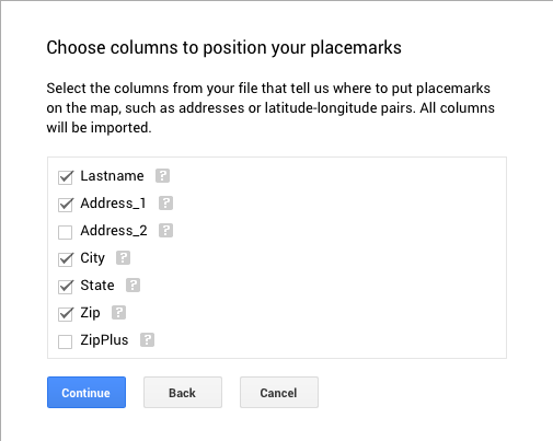
When the import completes, Google opens the Choose columns to position your placemarks box. Checkmark the boxes (e.g., name, address, city, state, zip) that are relevant for your data and then click Continue.
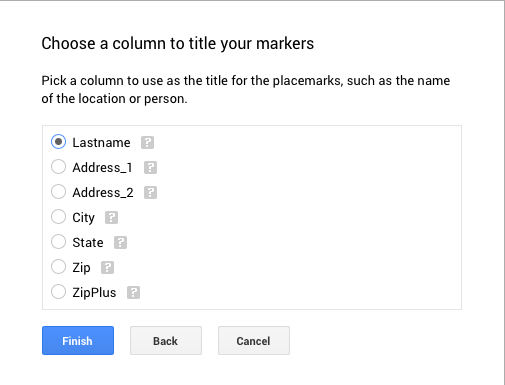
Now, in the Choose a column to title your markersbox, checkmark the appropriate box (for example, Lastname). The column you choose provides the title to the call-out information box that pops up when you click a marker on the map. Click Finish and Google completes importing your data.
EDITING ICONS
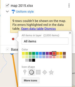
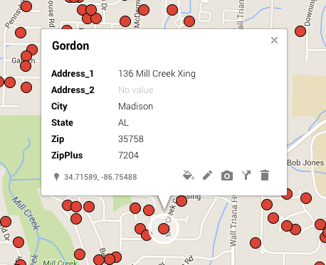
The resulting map should look familiar: Google’s iconic balloon icons saturate the map, each icon representing a row of your spreadsheet. If you want to change the icon, Google gives you some options. To access these, hover your mouse cursor over All itemsand click the paint bucket icon at the right end of the field. For my map, I changed the default balloon icon for a red dot.
A COUPLE PROBLEMS
That was easy. Easy, that is, unless your spreadsheet has location errors or it just plain confuses Google’s addressing software. You may see a warning in the new map box about rows with errors that Google is unable to display on the map. To correct, click Open data tableand either edit the offending data or delete the rows (if you can live without their data). Also, zoom out on the map and see if there are odd markers located where they shouldn’t be. For these, right-click on each marker and choose Delete.
Another data problem you may confront is that not all of your data was imported. As of this writing, Google Maps imports a maximum of 2000 addresses. This may require you to break your spreadsheet into two files and import both.
You can add more markers to your map by creating a new layer and entering an address (or, sometimes, the name of a point-of-interest) in the Search box to the right of the new map box. You can add your Google Map to your website by creating an iframe on the web page that links to the URL of your new Google Map.
For more information on Google Map’s Help page or try Reddit.
Most of our day-to-day databases include geographic data such as country, region, city, address, latitude-Longitude, place names, etc. Many of you are used to storing these data on spreadsheets applications like Google Sheets, Microsoft Excel, etc… If you can link these databases to a map, you can see the changes to your data in real time on the map. In this post, I will show you how you can link Google Sheets to Google Maps to view changes to Spreadsheet dynamically.
You may also be interested in How to generate static Google Maps in Google Sheets.
Though you can easily create a Google My Map by importing Google Sheets, you need to import it every time to see the changes to the Spreadsheet. You cannot refresh the map to apply changes to the Spreadsheet or do any sort and filtering etc…
However, if you create your map in Google Data Studio, you can get the benefits of many of its native features to enhance the functionality of your map. In this post, I will show you how you can use Google Data Studio to link Google Sheets to Google Maps.
If you haven’t used Google Data Studio before, I suggest you read “How to Create an Online Dashboard for free to Share and Visualize Your Data“.
Table of Contents
Benefits of Using Google Data Studio to Link Google Sheets to Google Maps
- Changes to your Google Sheets data are updated automatically on your map
- You can sort and filter your data and see the changes in real-time
- Customize your map layers
- Change bubble (marker) size & color
- Set bubble size to vary with the values
- You can plot many geographic dimensions (Eg. Address, City, Region, etc…) no need to provide coordinates every time
- Can have multiple maps in the same window
- Can use many other data sources
- Use many other data visualization elements to create a complete dashboard
- It’s completely free.
Limitations
There are also some limitations when linking Google Sheets to Google Maps using this method.
- At present, data can only be represented as bubbles
- Maximum Data Limits
- 10,000 bubbles for Latitude, Longitude fields.
- 1,000 bubbles for other geographic field types.
Step-by-step guide to linking Google Sheets to Google Maps in Google Data Studio
For this example, I use the “World Airports” data set downloaded from ArcGIS Hub
You can make a copy of the Google Sheet with the data from here.
You can see a live demo built with the above data set from this link.
Step 01: Prepare your Google Sheet (Data Sheet)
- Make sure your datasheet does not have merged cells.
- The first row should be your column headers.
- Each record should be represented by a single row.
- If you are using city names, country names, addresses, etc… make sure you don’t have any typos.
- The latitudes and longitudes should be in the form of [latitude, longitude]. If latitudes and longitudes are in separate columns, either;
- You can create a new column in your Google Sheet and combine latitude and longitude values. You can use the following array formula if A and B columns contain latitude and longitude values.
=ARRAYFORMULA(if(ISBLANK(A2:A),””,A2:A&”,”&B2:B)) - Or you can create a calculated field in Google Data Studio, as explained in the next step.
- You can create a new column in your Google Sheet and combine latitude and longitude values. You can use the following array formula if A and B columns contain latitude and longitude values.
Step 02: Create a new Data Source in Google Data Studio
- Open Google Data Studio.
- Click on
 Create button and select the Data source. If this is the first time you are using Data Studio, it will popup the configuration wizard and ask you to accept terms and conditions and to set up your preferences.
 - Click on the Google Sheets option.
- The next page shows up all the Google Sheets saved in your Google Drive. Select the correct Spreadsheet. (World Airports in this case)
- In the Worksheet column, select the worksheet with your data.
- Click the CONNECT button at the top right corner of the page.
- On the next page, you can rename your data source at the top left corner.
- Select the correct data type for each field.
- For your geographical fields, for example, if you have a country field, click the “type” cell next to your field name > hour over the Geo field > Select Country.
- As I mentioned in Step 01, you can create new fields using the exiting fields. To create the [Latitude, Longitude] field,
- Click Add A Field butting closer to the top right corner
- Type a field name (Eg. Latitude_Longitude)
- In the formula box type the following equation (assuming your existing field names are “latitude” and “longitude”)
CONCAT(latitude,CONCAT(“,”,longitude)) - Click SAVE
- Change the data type to Latitude, Longitude as explained above.
- Finally, click the CREATE REPORT button at the top right corner of your page.
Step 03: Add Google Maps to your Report
- Once you click the CREATE REPORT button, you are directed to the report page. It will automatically add a sample table using a few fields of your data set. Click and delete it if you do not want it.
- To add a Google Map, click Add a chart > Google Maps. Click somewhere in the report to place the map.
- Once you add the map, it will be populated with one of your Geodata fields.
- You can also add multiple maps on the same page.
Step 04: Customizing the Maps
- Click on the map to select it
- Customization options are in the right-side panel. In this panel, there are two tabs, namely Data and Style.
- Under the Dimension section in the Data tab
- For the Bubble location, select your Geo field.
- For the Tooltip, select the location name or any field that needs to appear when hour over the bubble.
- You can add different colors to your bubbles based on the unique data in the selected field. This is useful when you have a fever number of unique data. Add colors using the Bubble color field.
- Under the Metric section in the Data tab
- You can also set the bubble size to be varying with the value of your data. You can set it using the Bubble size field.
- In the style tab, there are many options that allow you to style the Background Layer, Bubble Layer, Colors, Map controls, Background and border, and Chart headers.
- For example; using the bubble layer, you can set the bubble size and the number of bubbles to be displayed.
Step 05: Add Filters and other Visual Elements
You can build a complete dashboard with Google Data Studio. Google Maps is only one visual element out of plenty of visual elements available on Data Studio. You can add these visual elements to create a dynamic map.
Add Filters Controls
You can use filter controls to, filter your data inside the map.
- Click the filter icon in the top menu and draw the filter box in the report.
- You can add multiple filter controls.
- Select all the related filter controls and the map.
- Right-click on the selected elements and click group.
Add other Visual Elements
You can also add other visual elements such as different types of graphs, tables, scorecards, etc… Follow the same method described above for adding filter controls when adding other elements also. You need to group all these related items.
Step 06: View the Map/ Dashboard
Your map is not interactive in the edit mode. Click the View button at the top right corner to switch to the view mode.
There are multiple ways that you can share your report.
- Invite people through their email addresses with a view or edit permission.
- Schedule email delivery – useful if your database is continuously updating
- Get the report link and share it.
- Embed report on your website (Google Map does not work on embedded reports)
- Download as a PDF
Wrapping Up
The Google Map feature of the Google Data Studio allows you to map valid geographic data in your database. You can easily connect your Google Sheets with Google Data Studio with a few clicks. These two features make a powerful environment where you can connect Google Sheets with Google Maps. The Google Maps feature of the Google Data Studio is highly customizable, and you can make use of the other Data Studio features to create an interactive map. Most importantly, Google provides all these features to you free of charge.
Accordingly, this post explains to you how you can link Google Sheets to Google Maps using Google Data Studio. However, the map you can build using this method is subject to some limitations, as mentioned above. The Google Maps feature is only one of the plenty of Google Data Studio features. By using all these features, you can build a feature-rich dashboard too.
References
- Data Studio Help
- Data Studio Help – Google Maps reference

Mapping Using Excel with Google Maps

Overview • To maximize time and mileage, we have everyone map out and plan their daily route. • We have found a way of using google maps and excel worksheets to improve this process. • You will need a google account to use the feature, so if you aren’t already using gmail or don’t have a google account, you will need to create one for free. That can be done here: https: //accounts. google. com/signup

Accessing Google Maps • There are different ways to access google maps: • You can type in the URL maps. google. com and if you are signed into your account, then it will open under your account automatically. • If you are already logged into your google account, you can click on the google apps icon at the top right of the screen (9 small boxes in a square shape) and select the “Maps” icon • This should open google maps and you will see a map with a search bar in the top left corner of the screen.

1. Click here 2. This menu should open 3. Click on the “Maps” icon

This screen should open:

Opening “My Maps” • Using your google account, you can create and save maps that you can later view, edit, etc. This is what we have done for each county to log in the farm, housing and community contact info that many of you have used. • We now want to show you can use the tool to map out your own routes using data compiled in an excel spreadsheet (current student addresses, old addresses, farm lists, etc. ). • You can create different layers on the map which show different categories such as old addresses, current addresses, and farm info. • You can even export the current data on a map we have made for a county and then add more layers for them like old addresses and current families- but more on that later.

Creating Your Own Google Map • Now that you have google maps open, click on the menu icon (three horizontal lines) at the top left corner of the screen. • The menu will open with many options. Click on the “My Maps” option.

1. Click here 2. This menu should open 3. Click on the “My Maps” icon

Accessing Saved Maps and Creating New Maps • If you have already saved maps, this is where you can access them. • You can also create a new map by clicking the “Create Map” option at the bottom. • For demonstration purposes, lets click on “Create Map”

Saved maps can be accessed here: You can create a new map by clicking here:

After Clicking “Create Map” this screen should appear

Editing Tool Bar-adding markers and drawing lines Search Bar: You can type an address, business, or other location, and it will be marked on your map with a place marker. Once added, you can change the name and format of the marker and add a description if you’d like. Select Items: The hand icon is the default tool and can be used to select icons that are already added or to move around the map by clicking and dragging. Add Marker: This can be used to mark a location on the map with a pin point if you want to mark a specific spot. This is helpful if you don’t know the address but know the location. Draw a Line: This feature is great for outlining a field or streets/housing area.

Map Menu and Using Layers Click here to edit map name: As mentioned earlier, you can add different layers to the map to show different types of items such as current housing, old addresses, and farms. You can title the different layers according to what is included in them as well by simply clicking on the text “Untitled Layer” You have two options for adding info to a layer. You can draw it using the tools shown on the previous slide (Adding a marker, drawing a line or shape) or you can import data from an excel sheet which we will look at next.

Importing Excel Spreadsheet to Google Maps • Click “Import” link in the layer where you want to add data. • You can drag or search for the file you want to import. The file must be a CVS, EXSL, KML or GPX File. • EXSL (Excel file) can be used to add in farm info as well as addresses. • KML is the type of file that can be exported from an existing map (such as those we have created with each county’s info) and then you can import them into your own map. More on that later.

Preparing Excel Files for Importing • Before importing a file, there are some things that need to be considered and possibly changed. • The excel file should only have one worksheet (one tab at the bottom). If there are more than 1 worksheet, it doesn’t import. • The excel file must include in at least one column the address info that you want to import to the map and then what you want the title of the place mark to be. • The first row of the worksheet must have a title for that column (Address, student name, farm name, etc. ) • *Note: If you want to use the student lists from the server, you must copy and past the info you want into a new spreadsheet and save that to upload to the map. I just copy all address info and student last names and paste into a new workbook and save it.

Here I have copied and pasted the Rows and Columns I want from the student list on the server, keeping the first row with column titles. I have saved the xlsx file. Now I want to import it into my map.

Importing Spreadsheet to Map Layer 1. In the map legend, select the layer you want to import your data to (there can be multiple layers although only one is shown here) 2. Click “import”

You can drag the file or search for it on you computer.

1. Choose Columns to position your place marks. 2. Choose a column to title your markers. Because I had the number, street, and city in different columns, I selected all three. If you have the address all in one column, you’d only need to select the one. I wanted to have the family’s last name as the title of each mark so I selected “Last Name 1. ” If it is a farm list you would select the column title where the farm’s name is.

If all was done correctly, the data should import to the map and when you click on each marker it will tell you the name of the location you selected.

Fixing Data Errors • Sometimes due to how the data is entered, google maps cannot add in an address you wanted (or several at times). • Also, some locations may be mapped in the wrong location (in a different state). • You can edit the information from the spreadsheet right in the map using the data table in the legend.

In the error message, click on open data table, and the data from the imported spreadsheet will open. Simply click in the field you want to edit and change the text. Typically, apt and lot numbers are not accepted and cannot be mapped. Also, if there are not spaces where they need to be, errors occur.

The data table can also be accessed and edited anytime by clicking the three vertical dots next to the layer title: This menu will then open. You can rename or delete the layer, or select open data table to edit info.

Exporting Existing Map info to Import into New Map • You may want to create your own map that includes the info we have added to each county’s google map and also other info like current or old addresses. • To do this, use the link for the google map you want to export info from to open the map.

Once the map is open, select the three dots in the legend. Be sure the layer with the info you want to export is selected. Then select “Export to KML. ” It will give you the option to export as a KML or a KMZ file. The only difference is a KML WON’T have the custom icons we use, and a KMZ will. This will automatically download the file to your computer.

Adding New Layer to your Map with Existing Map info You then follow the same process as you would for importing an excel file, but when choosing the file to upload and import you select the KML or KMZ file that was exported and downloaded from the existing map (in the downloads folder of your computer). Now there are two separate layers: one for the current addresses and another of existing map info.

Additional Comments • This is a great tool to help visualize and map out the county where you will be working. You can hide and show the different layers to see what is in which area and plan to go to locations based on proximity. • Maps are automatically saved as changes are made and are visible on the Google Maps App on phones and tablets. To access them on your phone, be sure you are signed into the google account you created the map with, open the maps app, select the menu (three horizontal lines at top left if using an android), and select “your places. ” The list of maps should be there. • *Reminder*- Do NOT rely solely on your phone in the field. ALWAYS have an accessible list off all the addresses you want to visit, current families in the area, and your plan for the day. This is a tool to help you plan your route AHEAD of time and can be used as a tool while in the field, but because areas we work in often do not have cell reception, a backup method is absolutely necessary.