
Excel for Microsoft 365 Excel for Microsoft 365 for Mac Excel for the web Excel 2021 Excel 2021 for Mac Excel 2019 Excel 2019 for Mac Excel 2016 Excel 2016 for Mac Excel 2013 Excel 2010 Excel 2007 Excel for Mac 2011 Excel Starter 2010 More…Less
You use the SUMIF function to sum the values in a range that meet criteria that you specify. For example, suppose that in a column that contains numbers, you want to sum only the values that are larger than 5. You can use the following formula: =SUMIF(B2:B25,»>5″)

This video is part of a training course called Add numbers in Excel.
Tips:
-
If you want, you can apply the criteria to one range and sum the corresponding values in a different range. For example, the formula =SUMIF(B2:B5, «John», C2:C5) sums only the values in the range C2:C5, where the corresponding cells in the range B2:B5 equal «John.»
-
To sum cells based on multiple criteria, see SUMIFS function.
Important: The SUMIF function returns incorrect results when you use it to match strings longer than 255 characters or to the string #VALUE!.
Syntax
SUMIF(range, criteria, [sum_range])
The SUMIF function syntax has the following arguments:
-
range Required. The range of cells that you want evaluated by criteria. Cells in each range must be numbers or names, arrays, or references that contain numbers. Blank and text values are ignored. The selected range may contain dates in standard Excel format (examples below).
-
criteria Required. The criteria in the form of a number, expression, a cell reference, text, or a function that defines which cells will be added. Wildcard characters can be included — a question mark (?) to match any single character, an asterisk (*) to match any sequence of characters. If you want to find an actual question mark or asterisk, type a tilde (~) preceding the character.
For example, criteria can be expressed as 32, «>32», B5, «3?», «apple*», «*~?», or TODAY().
Important: Any text criteria or any criteria that includes logical or mathematical symbols must be enclosed in double quotation marks («). If the criteria is numeric, double quotation marks are not required.
-
sum_range Optional. The actual cells to add, if you want to add cells other than those specified in the range argument. If the sum_range argument is omitted, Excel adds the cells that are specified in the range argument (the same cells to which the criteria is applied).
Sum_range
should be the same size and shape as range. If it isn’t, performance may suffer, and the formula will sum a range of cells that starts with the first cell in sum_range but has the same dimensions as range. For example:
range
sum_range
Actual summed cells
A1:A5
B1:B5
B1:B5
A1:A5
B1:K5
B1:B5
Examples
Example 1
Copy the example data in the following table, and paste it in cell A1 of a new Excel worksheet. For formulas to show results, select them, press F2, and then press Enter. If you need to, you can adjust the column widths to see all the data.
|
Property Value |
Commission |
Data |
|---|---|---|
|
$100,000 |
$7,000 |
$250,000 |
|
$200,000 |
$14,000 |
|
|
$300,000 |
$21,000 |
|
|
$400,000 |
$28,000 |
|
|
Formula |
Description |
Result |
|
=SUMIF(A2:A5,»>160000″,B2:B5) |
Sum of the commissions for property values over $160,000. |
$63,000 |
|
=SUMIF(A2:A5,»>160000″) |
Sum of the property values over $160,000. |
$900,000 |
|
=SUMIF(A2:A5,300000,B2:B5) |
Sum of the commissions for property values equal to $300,000. |
$21,000 |
|
=SUMIF(A2:A5,»>» & C2,B2:B5) |
Sum of the commissions for property values greater than the value in C2. |
$49,000 |
Example 2
Copy the example data in the following table, and paste it in cell A1 of a new Excel worksheet. For formulas to show results, select them, press F2, and then press Enter. If you need to, you can adjust the column widths to see all the data.
|
Category |
Food |
Sales |
|---|---|---|
|
Vegetables |
Tomatoes |
$2,300 |
|
Vegetables |
Celery |
$5,500 |
|
Fruits |
Oranges |
$800 |
|
Butter |
$400 |
|
|
Vegetables |
Carrots |
$4,200 |
|
Fruits |
Apples |
$1,200 |
|
Formula |
Description |
Result |
|
=SUMIF(A2:A7,»Fruits»,C2:C7) |
Sum of the sales of all foods in the «Fruits» category. |
$2,000 |
|
=SUMIF(A2:A7,»Vegetables»,C2:C7) |
Sum of the sales of all foods in the «Vegetables» category. |
$12,000 |
|
=SUMIF(B2:B7,»*es»,C2:C7) |
Sum of the sales of all foods that end in «es» (Tomatoes, Oranges, and Apples). |
$4,300 |
|
=SUMIF(A2:A7,»»,C2:C7) |
Sum of the sales of all foods that do not have a category specified. |
$400 |
Top of Page
Need more help?

See also
SUMIFS function
COUNTIF function
Sum values based on multiple conditions
How to avoid broken formulas
VLOOKUP function
Need more help?
The SUMIF function sums cells in a range that meet a single condition, referred to as criteria. The SUMIF function is a common, widely used function in Excel, and can be used to sum cells based on dates, text values, and numbers. Note that SUMIF can only apply one condition. To sum cells using multiple criteria, see the SUMIFS function.
Syntax
The generic syntax for SUMIF looks like this:
=SUMIF(range,criteria,[sum_range])The SUMIF function takes three arguments. The first argument, range, is the range of cells to apply criteria to. The second argument, criteria, is the criteria to apply, along with any logical operators. The last argument, sum_range, is the range that should be summed. Note that sum_range is optional. If sum_range is not provided, SUMIF will sum cells in the first argument, range.
Examples: Basic Usage | Criteria in another cell | Not equal to | Blank cells | Dates | Wildcards | Videos
Applying criteria
The SUMIF function supports logical operators (>,<,<>,=) and wildcards (*,?) for partial matching. The tricky part about using the SUMIF function is the syntax needed to apply criteria. This is because SUMIF is in a group of eight functions that split logical criteria into two parts, range and criteria. Because of this design, operators need to be enclosed in double quotes («»). The table below shows examples of the syntax needed for common criteria:
| Target | Criteria |
|---|---|
| Cells greater than 75 | «>75» |
| Cells equal to 100 | 100 or «100» |
| Cells less than or equal to 100 | «<=100» |
| Cells equal to «Red» | «red» |
| Cells not equal to «Red» | «<>red» |
| Cells that are blank «» | «» |
| Cells that are not blank | «<>» |
| Cells that begin with «X» | «x*» |
| Cells less than A1 | «<«&A1 |
| Cells less than today | «<«&TODAY() |
Notice the last two examples involve concatenation with the ampersand (&) character. Any time you are using a value from another cell, or using the result of a formula in criteria with a logical operator like «<«, you will need to concatenate. This is because Excel needs to evaluate cell references and formulas to get a value before that value can be joined with an operator.
Limitations
There are a couple of limitations with SUMIF that you should be aware of. First, SUMIF only supports a single condition. If you need to sum cells using multiple criteria, use the SUMIFS function. Second, the SUMIF function requires an actual range for the range argument; you can’t substitute an array. This means you can’t do things like extract the year from a range that contains dates inside the SUMIF function. If you need to manipulate values that appear in the argument before applying criteria, the SUMPRODUCT function is a flexible solution.
Basic usage
With numbers in the range A1:A10, you can use SUMIF to sum cells greater than 5 like this:
=SUMIF(A1:A10,">5")If the range B1:B10 contains color names like «red», «blue», and «green», you can use SUMIF to sum numbers in A1:A10 when the color in B1:B10 is «red» like this:
=SUMIF(B1:B10,"red",A1:A10)Notice A1:A10 is now entered as the sum_range, because it is different from range, which contains only color names. To recap: criteria is applied to cells in range. When cells in range meet criteria, corresponding cells in sum_range are summed. The sum_range argument is optional. If sum_range is omitted, the cells in range are summed instead.
Worksheet example
In the worksheet shown, there are three SUMIF formulas. In the first formula (G5), SUMIF returns total Sales where Name = «jim». In the second formula (G6), SUMIF returns total Sales where State = «ca» (California). In the third formula (G7), SUMIF returns the total of Sales > 100:
=SUMIF(B5:B15,"jim",D5:D15) // name = "jim"
=SUMIF(C5:C15,"ca",D5:D15) // state = "ca"
=SUMIF(D5:D15,">100") // sales > 100
Notice the equals sign (=) is not required when constructing «is equal to» criteria. Also notice SUMIF is not case-sensitive; you can use «jim» or «Jim». Finally, notice that the last formula does not include sum_range, so range is summed instead.
Criteria in another cell
A value from another cell can be included in criteria using concatenation. In the example below, SUMIF will return the sum of all sales over the value in G4. Notice the greater than operator (>), which is text, must be enclosed in quotes. The formula in G5 is:
=SUMIF(D5:D9,">"&G4) // sum if greater than G4

Not equal to
To express «not equal to» criteria, use the «<>» operator surrounded by double quotes («»):

=SUMIF(B5:B9,"<>red",C5:C9) // not equal to "red"
=SUMIF(B5:B9,"<>blue",C5:C9) // not equal to "blue"
=SUMIF(B5:B9,"<>"&E7,C5:C9) // not equal to E7
Again notice SUMIF is not case-sensitive.
Blank cells
SUMIF can calculate sums based on cells that are blank or not blank. In the example below, SUMIF is used to sum the amounts in column C depending on whether column D contains «x» or is empty:

=SUMIF(D5:D9,"",C5:C9) // blank
=SUMIF(D5:D9,"<>",C5:C9) // not blank
Dates
The best way to use SUMIF with dates is to refer to a valid date in another cell, or use the DATE function. The example below shows both methods:

=SUMIF(B5:B9,"<"&DATE(2019,3,1),C5:C9)
=SUMIF(B5:B9,">="&DATE(2019,4,1),C5:C9)
=SUMIF(B5:B9,">"&E9,C5:C9)
Notice we must concatenate an operator to the date in E9. To use more advanced date criteria (i.e. all dates in a given month, or all dates between two dates) you’ll want to switch to the SUMIFS function, which can handle multiple criteria.
Wildcards
The SUMIF function supports wildcards, as seen in the example below:

=SUMIF(B5:B9,"mi*",C5:C9) // begins with "mi"
=SUMIF(B5:B9,"*ota",C5:C9) // ends with "ota"
=SUMIF(B5:B9,"????",C5:C9) // contains 4 characters
The tilde (~) is an escape character to allow you to find literal wildcards. For example, to match a literal question mark (?), asterisk(*), or tilde (~), add a tilde in front of the wildcard (i.e. ~?, ~*, ~~).
Average range caution
SUMIF makes certain assumptions about the size of sum_range, essentially resizing it when necessary to match the range argument, using the upper left cell in the range as an origin. In some cases, this behavior can create a result that seems reasonable but is in fact incorrect. For an example of this problem, see this article.
Notes
- SUMIF only supports one condition. Use the SUMIFS function for multiple criteria.
- When sum_range is omitted, the cells in range will be summed.
- Non-numeric criteria must be enclosed in double quotes (i.e. «<100», «>32», «TX»)
- Cell references in criteria are not enclosed in quotes, i.e. «<«&A1
- The wildcard characters ? and * can be used in criteria. A question mark matches any one character and an asterisk matches any sequence of characters (zero or more).
- To match a literal question mark(?) or asterisk (*), use a tilde (~) like (~?, ~*).
- SUMIF requires a range, you can’t substitute an array.
Adding up all the numbers in a single column or row in Excel is easy — the SUM function will work just fine. But what if you only want to sum cells that meet a certain condition – for example, to calculate the total sales generated by a specific product? In this case, Excel has a useful function called SUMIF to help you with the job!
Now, let’s go over what the SUMIF function is and how to use it with various examples, so you can see just how helpful this tool can be!
What is the SUMIF function in Excel?
The SUMIF function is a perfect choice when you’re looking for an easy way to aggregate certain data quickly. Unlike pivot tables, which may require more advanced knowledge in order to use correctly, SUMIF is relatively easy to get started with.
Here we have a spreadsheet that shows how much revenue was generated by each product and its packaging:
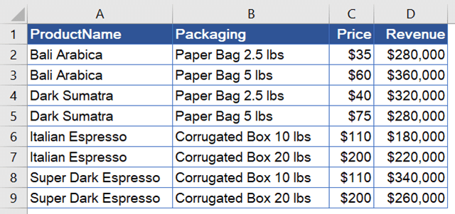
As you’re looking at the above data, the following questions might cross your mind:
- What is the total revenue generated by Bali Arabica?
- What is the total revenue generated from products with prices under $50?
- What is the total revenue generated from products packaged in paper bags?
The SUMIF function can help you answer those questions quickly. With it, you can sum values based on a single criteria, like those specified by the above questions.
Can I use SUMIF with multiple criteria?
SUMIF does not support multiple criteria. For example, you can’t use it to answer questions like: “What is the total revenue generated by products with paper bag packaging AND prices under $50?“. To work around this limitation, you’ll need to use the SUMIFS function, which is the more advanced version of SUMIF.
So, while SUMIF in Excel is powerful and easy to use, it does have its limitations. For that reason, you will find several examples in this article using SUMIFS as well as other functions as a workaround for solving cases that cannot be solved using SUMIF.
Excel SUMIF syntax and parameters
Syntax
=SUMIF(critera_range, criteria, [sum_range])Parameters or arguments
| Parameters | Description |
|---|---|
criteria_range |
Required. The range of cells that contains the criteria. |
criteria |
Required. The criteria used to determine which cells to add. It can be in the form of a number, expression, cell reference, text, or function.
Note: You need to use double quotation marks around any text criteria that include logical or mathematical symbols. If the criteria are numeric, you don’t need double quotes. You can also use logical operators as well as wildcards for partial matching, which makes the function powerful. Wildcards: – An asterisk ( – A tilde ( |
[sum_range] |
Optional. The range of cells to add. If you don’t specify this argument, Excel adds the cells that are specified in the criteria_range argument. |
How to use SUMIF in Excel: Basic usage
To have a good understanding of how to use the SUMIF function in Excel, let’s take a look at an example below. Suppose you want to find the total revenue generated by Bali Arabica, and want to store the result in G3.

To do that, follow the steps below:
Step 1: Position your cursor on G3 and start entering the formula.
=SUMIF(
Step 2: Enter the range of cells that contains the criteria, which is A2:A9.
=SUMIF(A2:A9
Step 3: Set your criteria in the second argument by typing "Bali Arabica".
=SUMIF(A2:A9,"Bali Arabica"
Note: You can type
"bali arabica"or"BALI ARABICA"because SUMIF is not case-sensitive. You can also add the “=” operator in the criteria ("=Bali Arabica"), but the equal sign (=) is not necessarily required when creating the “is equal to” criteria.
Step 4: Select a range of cells that you want to sum, which is D2:D9. After that, close the parentheses and press Enter.
=SUMIF(A2:A9,"Bali Arabica", D2:D9)

Let’s see what exactly happened:
- Excel searched for the word “Bali Arabica” in the range A2:A9
- If any row had that word, Excel added the revenue value in column D of the same row.
- In the end, you get the sum of all revenue for Bali Arabica.
Note: If your spreadsheet has many rows, using this formula that refers to the entire column may be more convenient:
=SUMIF(A:A,"Bali Arabica",D:D)
Now, if you’d like, try to calculate the revenue generated from Dark Sumatra, Italian Espresso, and Super Dark Espresso. You can follow the same steps as above (Step 1-4).
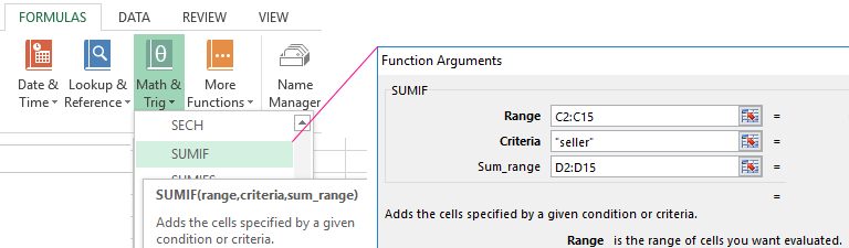
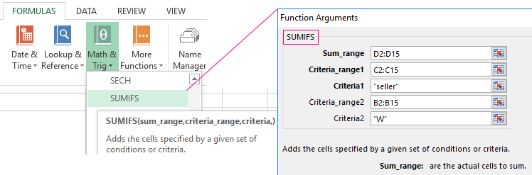
Alternatively, you can insert the SUMIF formula from the ribbon menu. To do that, click Formula, and then in the Function Library section, click Math & Trig. Look for the SUMIF function in the list and select it.

A popup will appear, allowing you to enter the function arguments. See the following arguments for Dark Sumatra. When done, click the OK button.

Excel SUMIF vs. SUMIFS
When talking about SUMIF, we really must also discuss SUMIFS. Both functions allow you to sum data based on certain conditions. The difference? SUMIF only supports a single criteria, whereas SUMIFS can handle multiple criteria.
SUMIFS syntax
=SUMIFS(sum_range, criteria_range1, criteria1, [criteria_range2, criteria2], …)The syntax is different from SUMIF in that you need to include the sum_range argument before any other arguments. Also, sum_range is a required argument, not optional like in the SUMIF function. Following the sum_range argument is the pair of the first criteria range and criteria (criteria_range1 and criteria1), and this pair of parameters is also required.
You can use SUMIFS even for one criteria (like SUMIF). You can add as many criteria as necessary, up to the limit of 127 pairs.
The basics of how to use these parameters are the same as SUMIF, so we won’t repeat the same explanation here. That means you won’t have to read a longer 😉
How to use SUMIF in Excel if your data is from different sources
Have you ever wanted to analyze data using Microsoft Excel, but your data is stored in external sources such as Jira, PipeDrive, Shopify, etc.? If yes, but you just couldn’t figure out how, our integration tool, Coupler.io, can help you. With this tool, you can import and combine data from different sources into Excel without coding. You can even automate the process on a schedule!
It’s important to note that your destination file needs to be an Excel Online file on OneDrive. If you want to use a file shared by another user, ensure you have edit access to the file.
To start using Coupler.io, sign up to it (it’s easy and no credit card is required). Then, all you need to do is create a new importer. A wizard will help you configure these three details:
- Source — You can take data from Airtable, Xero, Slack, Trello, and more.

- Destination — Select Microsoft Excel.

- Schedule— If you’d like, you can set up automatic data refresh on a schedule: hourly, daily, or monthly.

Pretty easy, right?! Once you finish setting up the importer and run it, your Excel file will be updated. Check out the available Excel integrations.
After that, you can start analyzing your data using Excel. 🙂
Common examples of how to use the SUMIF function in Excel
Understanding the basic use of SUMIF is one thing. But it’s better to be aware that there are many different ways to use this function. Now, let’s look at some common examples so we can get an idea of other fun things we can do with this function.
#1: Excel SUMIF if cells are equal to a value in another cell
With the data below, suppose you want to find out how many items were sold at $200. You can use this formula:
=SUMIF(B2:B9,200,C2:C9)
But instead of typing 200 manually as the second parameter, you can just refer to E3, as shown in the following formula:
=SUMIF(B2:B9,E3,C2:C9)

#2: If cells are not equal to
To calculate using the “not equal to” criteria, use the “<>” operator (with double quotes).
Now, assume that you want to calculate the total sales generated by products other than Rose in E3 and other than Daisy in E4. Use the following formulas:
- Not equal to Rose (E4):
=SUMIF(A2:A6,"<>Rose",B2:B6)
- Not equal to Daisy (E5):
=SUMIF(A2:A6,"<>"&D4,B2:B6)
Notice that for Daisy, we use a cell reference in the formula.

#3: If cells are less than / less than or equal to a number
Use the “<” operator to mean “less than” and “<=” to mean “less than or equal to“. The following example calculates the quantities of flowers with prices per stem that are:
- Less than $0.45 (F5):
=SUMIF(B2:B9,"<0.45",C2:C9)
- Less than or equal to $0.45 (F6):
=SUMIF(B2:B9,"<=0.45",C2:C9)

#4: If cell contains text
To sum if cells contain a specific text, you need to use a wildcard when specifying the criteria in the SUMIF function.
The following example calculates the total quantities of flowers with names containing “white“. Notice again that SUMIF is not case-sensitive. The formula in F5:
=SUMIF(A2:A9,"*white*",C2:C9)

#5: Excel SUMIF if cells contain an asterisk
Asterisks themselves are wildcards. So, to find text that contains an asterisk, you’ll need to use a tilde (~) to treat the character literally (not as a wildcard). The following example shows how to sum the amount for items that:
- Contain * (F5):
=SUMIF(B2:B9, "*~**", C2:C9)
- Contain * at the end (F6):
=SUMIF(B2:B9,"*~*",C2:C9)

#6: Excel SUMIF to sum values based on cells that are blank
Use double quotes without any space in between ("") in the criteria if you want to sum based on cells that are blank. Blank means empty or zero character length.
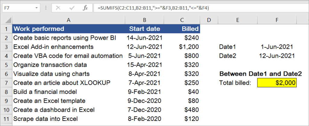
For the following spreadsheet, suppose you want to calculate the total bill for works that are still ongoing (not finished yet). To do that, you calculate the sum based on the finish dates that are blank using the following formula:
=SUMIF(C2:C11,"", D2:D11)

#7: Excel SUMIF to sum values based on cells that are not blank
Use the “not equal to” operator enclosed with double quotes (“<>“) in the criteria if you want to sum based on cells that are not blank.
Now, suppose you want to calculate the total bill only for works that are done (finish dates are not empty), use the following formula:
=SUMIF(C2:C11,"<>",D2:D11)

#8: If date is greater than, greater than or equal to
Use the “>” operator for greater than and “>=” for greater than or equal to. The following example sums the total bill for works that started:
- After Jun 5, 2021 (F5):
=SUMIF(B2:B11,">6/5/2021",C2:C11)
- On or after Jun 5, 2021 (F6):
=SUMIF(B2:B11,">="&DATE(2021,6,5),C2:C11)
Notice the formula in F6. You can also use the DATE function in the criteria.

Check out our guide dedicated to Excel SUMIF with Date Criteria.
#9: Excel SUMIF to sum values with the time format
Excel time values are actually numbers and you can sum them up using the SUMIF function like other numeric values. All you need to do is ensure that your data is in the correct time format. But how to set the correct time format? Well, it’s easy. Here’s an example:
Suppose you want to format Duration (column C) so that it uses the “h:mm:ss” format as shown in the following screenshot:

Follow the simple steps below:
Step 1: Select the entire column C (or only C2:C14 if you want to select this range only).
Step 2: Right-click and select Format Cells.
Step 3: Click Custom in the category list, then select h:mm:ss on the right.
Step 4: Click OK.
Now, let’s say you want to sum the total duration for Specialization 2. You can use the following formula:
=SUMIF(A2:A14,E4,C2:C14)

Note: When the sum of time can be greater than 24 hours, you should format the result cells to [h]:mm:ss to avoid the wrong total hours displayed in the results. That’s because for the normal time format like “h:mm:ss”, hours will reset to zero every 24 hours.
#10: With multiple OR criteria
To sum numbers based on other cells being equal to either one value or another, one of the solutions is by using multiple SUMIF functions in one formula.
With the following table, suppose you want to sum the quantity sold for either Orchid OR Sunflower. To do that, you can use the following formula:
=SUMIF(B2:B9,"Orchid",C2:C9)+SUMIF(B2:B9,"Sunflower",C2:C9)
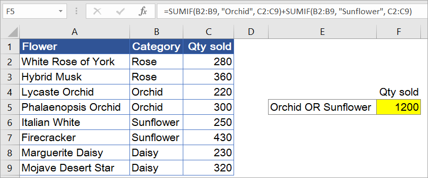
The solution here is very simple, and when there are only a few criteria, it often gets the job done quickly. However, if you want to sum values with more than three OR conditions (let’s say), then the formula will become long and complex. To avoid this problem, check out example #11 below, which uses a more advanced method that does not require adding up all of those different parts separately in order to get your total value.
Advanced examples of how to use the SUMIF function in Excel + without Excel SUMIF
Here are some more examples you may find helpful when summing values with criteria.
#11: Excel SUMIF with an array as the criteria argument
With the following data, suppose you want to sum the quantity sold for either Orchid OR Sunflower.

Notice that it uses multiple OR criteria, like in example #10. But this time, we’ll use an array in the criteria by following the steps below:
Step 1: List each condition separated by a comma and then enclose with curly brackets: {"Orchid","Sunflower"}
Step 2: Write the complete SUMIF formula using the array:
=SUMIF(B2:B9, {"Orchid","Sunflower"},C2:C9)
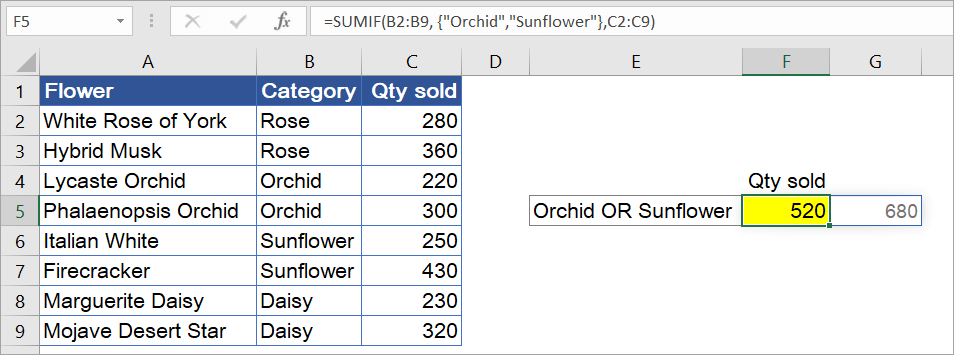
However, when you look at the result, the value is not correct. It only sums the total for Orchid, which is 520. And you’ll also see 680 next to it, which is the total for Sunflower. Why?
The SUMIF formula takes on an array argument that consists of two values. This forces the formula to return two results separately: 520 and 680. Since we put the formula in cell F5, the function only returns one result for this cell — i.e., the total for Orchid.
For this technique to work, you have to use one more step:
Step 3: Wrap your SUMIF formula in a SUM function, as follows:
=SUM(SUMIF(B2:B9, {"Orchid","Sunflower"},C2:C9))
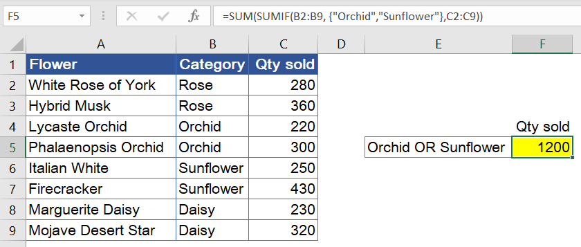
As you can see, the array criteria make the formula much more compact compared to multiple SUMIFs, as seen in example #10. You can also use arrays with numbers, but you don’t need to double-quote them.
#12: With date range criteria (between two dates)
Unfortunately, the SUMIF Excel formula does not work for this case. Instead, you have to use SUMIFS.
With the following data, suppose you want to sum the total bill for works started between 1-Jun-2021 (cell F3) and 12-Jun-2021 (cell F4). Use the formula below:
=SUMIFS(C2:C11,B2:B11,">="&F3,B2:B11,"<="&F4)
#13: Excel SUMIF by month
Suppose you have the following table and want to find the total bill for works that started in June 2001. To get the result, you can use a SUMIFS function with these two criteria: start dates >= first day of June AND start dates <= last day of June.

Follow the steps below:
Step 1: Type the first date of June 2021 in E3.

Step 2: Change the format of E3 to “mmmm” to display the month name.

Step 3: Write the following formula to F3, then press Enter. Note: The EOMONTH function helps you to find the last day of the month.
=SUMIFS(C2:C11, B2:B11, ">="&E3,B2:B11,"<="&EOMONTH(E3,0))

#14: Excel SUMIF by year
Still using the same data with the previous example, suppose you want to find the total bill for works that started in 2020. To get the result, use SUMIFS with these two criteria: start dates >= first day of 2020 AND start dates <= last day of 2020.
=SUMIFS(C2:C11, B2:B11, ">="&DATE(E3,1,1),B2:B11,"<="&DATE(E3,12,31))

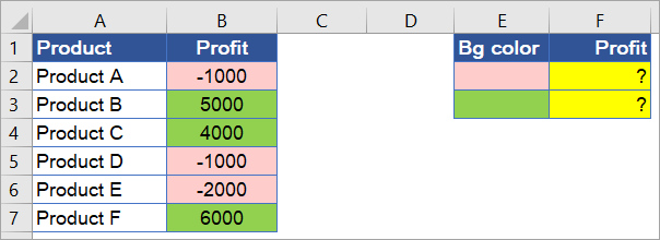
#15: Sum values based on background color
Suppose you have the following profit/loss data and want to sum based on the background color. In Excel, there is no default function to do that. But you can create an Excel VBA function to return the color index of a cell, and then use that index as the criteria in SUMIF.
Follow the steps below:
Step 1: Press Alt+F11 to open the Visual Basic Editor (VBE).
Step 2: Click Insert > Module.

Step 3: Copy-paste the following function to the editor:
Function ColorIndex(CellColor As Range)
    ColorIndex = CellColor.Interior.ColorIndex
End Function

Step 4: Type “Bg Color” as the header of column C. Then, type =ColorIndex(B2) in C2 and copy the formula down to C7.

Step 5: Use SUMIF to calculate the total profit based on the background color, as follows:
- Formula in F2:
=SUMIF(C2:C7, 19, B2:B7)
- Formula in F3:
=SUMIF(C2:C7, 43, B2:B7)

Read our guide on Excel SUMIFS VBA.
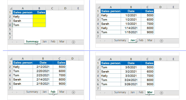
#16: Excel SUMIF to sum across multiple sheets
Suppose you have identical ranges in separate worksheets and want to summarize the total in the first worksheet, as shown in the following screenshot:
To do that, you can use the SUMIF function with INDIRECT, wrapped in SUMPRODUCT.
See the below steps to calculate the summary for the first salesperson (Kelly):
Step 1: List all the sheet names that are going to be summed in the Summary sheet. For example, in E2:E4 as shown below:
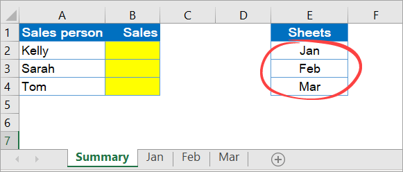
Step 2: Write a SUMIF formula for one sheet only – for example, Jan.
=SUMIF(Jan!A2:A6,Summary!A2,Jan!C2:C6)

Step 3: Nest the formula inside SUMPRODUCT.
=SUMPRODUCT(SUMIF(Jan!A2:A6,Summary!A2,Jan!C2:C6))
Step 4: Replace the sheet reference with a list of sheet names. In this case,
- Replace
Jan!A2:A6withINDIRECT("'"&E2:E4&"'!"&"A2:A6") - Replace
Jan!C2:C6withINDIRECT("'"&E2:E4&"'!"&"C2:C6")
The complete formula will be:
=SUMPRODUCT(SUMIF(INDIRECT("'"&E2:E4&"'!"&"A2:A6"),Summary!A2,INDIRECT("'"&E2:E4&"'!"&"C2:C6")))

#17: Sum multiple columns using one criteria
With the following data, suppose you want to calculate how many roses were sold in three months — Jan, Feb, and Mar. You can’t use either SUMIF or SUMIFS in this case. One alternative is to use the SUMPRODUCT function, as follows:
=SUMPRODUCT((A3:A11="Rose")*(B3:D11))

The first expression checks the range A3:A11 and returns an array of TRUE and FALSE. If any cell equals “Rose“, it will return TRUE, otherwise FALSE:
{TRUE;FALSE;FALSE;FALSE;FALSE;TRUE;TRUE;FALSE;FALSE}
The result above is then multiplied by the values in range B3:D11:
{500,400,300;400,500,200;500,300,400;300,400,500;400,200,500;400,500,200;600,200,300;400,300,200;400,500,300}
The SUMPRODUCT function will calculate the following values, which finally returns 3400.
=SUMPRODUCT({500,400,300;0,0,0;0,0,0;0,0,0;0,0,0;400,500,200;600,200,300;0,0,0;0,0,0})
Limitations of the Excel SUMIF function
After looking at these examples, we are sure you have your own conclusion about the limitations of the SUMIF function. But anyway, here’s the summary:
- You can’t use Excel SUMIF with multiple AND criteria. SUMIF is designed to handle one criteria only. As shown in example #10, you can use SUMIF + SUMIF for multiple OR conditions. However, you can’t use it with multiple AND criteria. For this case, use SUMIFS instead.
- You can’t use Excel SUMIF to sum multiple columns at once. As demonstrated in example #17, you can’t use either SUMIF and SUMIFS to sum multiple columns using one criteria. One of the solutions is to use the SUMPRODUCT function.
- You can’t use Excel SUMIF with an array as its range argument. In example #11, you can see that SUMIF accepts an array in its criteria argument. However, for its range argument, SUMIF requires a cell range. Because of this, you can’t use a formula that returns an array in its range argument — here’s an example:
Suppose you have the following table and want to sum the total bill for works that started in 2020; you can’t use this formula:
=SUMIF(TEXT(B2:B11,"yyyy"),"2020",C2:C11)

Why? That’s because the TEXT function in the above formula will return an array, which SUMIF doesn’t support.
What to do when your Excel SUMIF function is not working
There are times when you’ll find that your SUMIF formula in Excel is not working, or returns inaccurate results. There can be many reasons for that. Most of them have to do with incorrect ranges and defining criteria incorrectly. Thus, we recommend checking the following points:
- Check the order of the arguments used in the formula. For example, if you use three arguments, remember the first argument is the range that contains criteria, not the range you want to sum. You might have confused this with the SUMIFS formula.
- Check the range of cells you use, especially if you copy-pasted the formula from another cell. These include the range you want to sum as well as the range that contains the criteria.
- Ensure that you use double quotation marks (“”) for any criteria other than numeric.
- Check the format of the values involved in the calculation. For example, if you sum values with the time format, ensure you use the correct time format for your range values and the result cells.
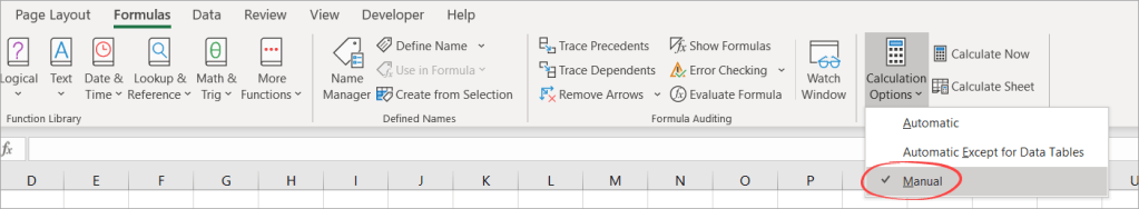
- You are sure that you’ve written the correct formula. Still, when you update the sheet, the SUMIF function doesn’t return the updated value? Well, in this case, check the formula calculation option in your spreadsheet. If it’s set to manual, press the F9 key to recalculate the sheet.
Finally, you’ve learned about the SUMIF function, including what it is, its syntax, how to use it, and its differences with SUMIFS. We also have covered various examples, as well as what to do when your function is not working.
We hope this article helped you, but if it didn’t, let us know if you have any comments or suggestions in the comments section below.
-

Senior analyst programmer

Back to Blog
Focus on your business
goals while we take care of your data!
Try Coupler.io

This Excel tutorial explains how to use the Excel SUMIF function with syntax and examples.
Description
The SUMIF function is a worksheet function that adds all numbers in a range of cells based on one criteria (for example, is equal to 2000).
The SUMIF function is a built-in function in Excel that is categorized as a Math/Trig Function. It can be used as a worksheet function (WS) in Excel. As a worksheet function, the SUMIF function can be entered as part of a formula in a cell of a worksheet.
To add numbers in a range based on multiple criteria, try the SUMIFS function.
![]() Subscribe
Subscribe
If you want to follow along with this tutorial, download the example spreadsheet.
Download Example
Syntax
The syntax for the SUMIF function in Microsoft Excel is:
SUMIF( range, criteria, [sum_range] )
Parameters or Arguments
- range
- The range of cells that you want to apply the criteria against.
- criteria
- The criteria used to determine which cells to add.
- sum_range
- Optional. It is the range of cells to sum together. If this parameter is omitted, it uses range as the sum_range.
Returns
The SUMIF function returns a numeric value.
Applies To
- Excel for Office 365, Excel 2019, Excel 2016, Excel 2013, Excel 2011 for Mac, Excel 2010, Excel 2007, Excel 2003, Excel XP, Excel 2000
Type of Function
- Worksheet function (WS)
Example (as Worksheet Function)
Let’s explore how to use SUMIF as a worksheet function in Microsoft Excel.
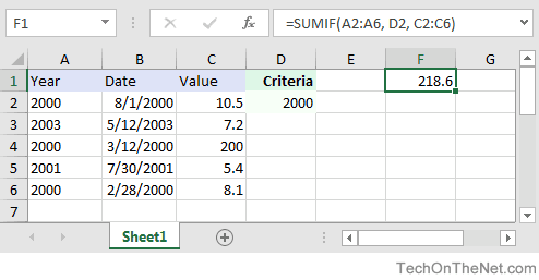
Based on the Excel spreadsheet above, the following SUMIF examples would return:
=SUMIF(A2:A6, D2, C2:C6)
Result: 218.6   'Criteria is the value in cell D2

=SUMIF(A:A, D2, C:C)
Result: 218.6   'Criteria applies to all of column A (ie: A:A)

=SUMIF(A2:A6, 2003, C2:C6)
Result: 7.2     'Criteria is the number 2003

=SUMIF(A2:A6, ">=2001", C2:C6)
Result: 12.6    'Criteria is greater than or equal to 2001

=SUMIF(C2:C6, "<100")
Result: 31.2    'Adds values in C2:C6 that are less than 100 (3rd parameter is omitted)
Now, let’s look at the example =SUMIF(A2:A6, D2, C2:C6) that returns a value of 218.6 and take a closer look why.
First Parameter
The first parameter in the SUMIF function is the range of cells that you want to apply the criteria against.
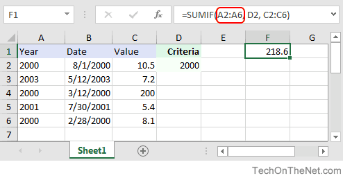
In this example, the first parameter is A2:A6. This is the range of cells that will be tested to determine if they meet the criteria.
Second Parameter
The second parameter in the SUMIF function is the criteria that will be applied against the range, A2:A6.
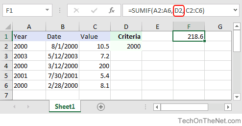
In this example, the second parameter is D2. This is a reference to the cell D2 which contains the numeric value, 2000. The SUMIF function will test each value in A2:A6 to see if it is equal to 2000.
Third Parameter
The third parameter in the SUMIF function is the range of numbers that will potentially be added together.
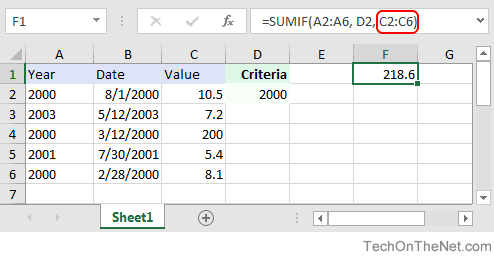
In this example, the third parameter is C2:C6. For every value in A2:A6 that matches D2, the corresponding value in C2:C6 will be summed.
Using Named Ranges
You can also use a named range in the SUMIF function. A named range is a descriptive name for a collection of cells or range in a worksheet. If you are unsure of how to setup a named range in your spreadsheet, read our tutorial on Adding a Named Range.
For example, if we created a named range called years in our spreadsheet that refers to cells A2:A6 in Sheet1 (Notice that the named range is an absolute reference that refers to =Sheet1!$A$2:$A$6 in the image below):
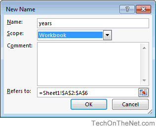
We could use this named range in our current example.
This would allow us to replace A2:A6 as the first parameter with the named range called years, as follows:
=SUMIF(A2:A6, D2, C2:C6)    'First parameter uses a standard range
Result: 218.6

=SUMIF(years, D2, C2:C6)    'First parameter uses a named range called years
Result: 218.6
Frequently Asked Questions
Question: I have a question about how to write the following formula in Excel.
I have a few cells, but I only need the sum of all the negative cells. So if I have 8 values, A1 to A8 and only A1, A4 and A6 are negative then I want B1 to be sum(A1,A4,A6).
Answer: You can use the SUMIF function to sum only the negative values as you described above. For example:
=SUMIF(A1:A8,"<0")
This formula would sum only the values in cells A1:A8 where the value is negative (ie: <0).
Question:In Microsoft Excel I’m trying to achieve the following with IF function:
If a value in any cell in column F is «food» then add the value of its corresponding cell in column G (eg a corresponding cell for F3 is G3). The IF function is performed in another cell altogether. I can do it for a single pair of cells but I don’t know how to do it for an entire column. Could you help?
At the moment, I’ve got this:
=IF(F3="food"; G3; 0)
Answer:This formula can be created using the SUMIF formula instead of using the IF function:
=SUMIF(F1:F10,"=food",G1:G10)
This will evaluate the first 10 rows of data in your spreadsheet. You may need to adjust the ranges accordingly.
I notice that you separate your parameters with semi-colons, so you might need to replace the commas in the formula above with semi-colons.
На чтение 2 мин
Функция СУММЕСЛИ (SUMIF) в Excel используется для суммирования значений, отвечающих заданным вами критериям.
Содержание
- Что возвращает функция
- Синтаксис
- Аргументы функции
- Дополнительная информация
- Примеры использования функции СУММЕСЛИ в Excel
Что возвращает функция
Возвращает сумму чисел, указанных в качестве аргументов и отвечающих заданным в формуле критериям.
 Больше лайфхаков в нашем Telegram Подписаться
Синтаксис
=SUMIF(range, criteria [sum_range]) — английская версия
=СУММЕСЛИ(диапазон; условие; [диапазон_суммирования]) — русская версия
Аргументы функции
- range (диапазон) — диапазон ячеек, по которым оцениваются критерии. Аргументом могут быть числа, текст, массивы или ссылки, содержащие числа;
- criteria (условие) — критерии, которые проверяются по указанному диапазону ячеек и определяют, какие ячейки суммировать;
- sum_range (диапазон_суммирования) — (не обязательно) суммируемые ячейки. Если этот аргумент не указан, то функция использует аргумент range (диапазон) в качестве sum_range (диапазон_суммирования).
Дополнительная информация
- суммирование ячеек в функции СУММЕСЛИ производится на основе одного критерия, если вам необходимо указать несколько критериев — используйте функцию SUMIFS (СУММЕСЛИМН);
- пустые и текстовые ячейки в аргументе sum_range (диапазон_суммирования) игнорируются;
- критерием для функции могут служить числа, выражения, результаты вычисления из других ячеек, текст или формула;
- если в качестве критерия указан текст или математический/логический символ (=,+,-,/,*), то такие значения должны быть указаны в двойных кавычках;
- аргумент с критерием не должен быть длиннее чем 255 символов;
- в качестве критерия могут использоваться подстановочные знаки (*);
- если количество ячеек в диапазоне критерия и аргументе sum_range (диапазон_суммирования) различаются, то размер диапазона критерия будет в приоритете.
Примеры использования функции СУММЕСЛИ в Excel
Probably everyone can summarize data in Excel program. But with the improved version of the SUM function, which is called SUMIF, the capabilities of this operation are significantly expanded.
By the name of the function, you can understand that it does not only calculate the sum, but also complies with some logical conditions.
SUMIF and its syntax
The SUMIF function allows you to sum cells that meet a certain criterion (a given condition). The arguments of the function are as follows:
- Range — cells, which should be evaluated on the basis of the criterion (the specified condition).
- Criteria, determining which cells from the range will be selected (written in quotation marks).
- Sum range — the actual cells that are needed to be summed if they meet the criterion.
Consequently the function has only 3 arguments. However, sometimes the third one can be excluded, and then the command will work only by the range and criteria.
How does the SUMIF function work in Excel?
Let’s consider the simplest example, which will clearly demonstrate how to use the SUMIF function and how convenient it can be for solving certain tasks.
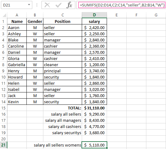
We have a table in which the names of employees, their gender and salary, calculated for January are indicated. If we just need to calculate the total amount of money that is required to pay out to employees, we use the SUM function, specifying all salaries by the range.
But what do we have to do if we need to quickly calculate only sellers’ salaries? In this case, the use of the SUMIF function will help.
Enter the arguments.
- The range in this case will be a list of all staff posts, because we will need to determine the whole amount of salaries. Therefore, enter E2:E14.
- The criterion of choice in our case is the seller. Enclose the word in quotation marks and put it as the second argument.
- The range of summation is salaries, because we need to know the amount of salaries of all sellers. Therefore, enter F2:F14.
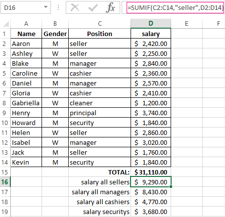
We have obtained 9290$. It means that the function automatically elaborated the list of all posts, chose only sellers from them and summed up their salaries.
Similarly, you can calculate the salaries of all managers, vendors, cashiers and security guards. When the table is small, it seems that everything can be counted manually, but when working with lists having several hundreds of positions, it makes sense to use SUMIF function.
SUMIF function in Excel with multiple criteria SUMIFS
If the letter S is added to the end of the standard SUMIF command, then it implies the function with several criteria (SUMIFS function). It is used in the case when you need to specify more than one criterion.
Syntax of using the function by several criteria
There can be as many arguments for SUMIFS as you like, but no less than 5.
- Sum range. If in SUMIF it was at the end, then here it is in the first place. It also indicates the cells that need to be summed.
- Criteria range 1 — cells that need to be evaluated on the basis of the first criterion.
- Criteria 1 — defines the cells that the function will select from the first range of the condition.
- Criteria range 2 — cells, which should be evaluated on the basis of the second criterion.
- Criteria 2 — defines the cells that the function will select from the second condition range.
And so on. Depending on the number of criteria, the number of arguments can increase in an arithmetic progression in step 2. That is, 5, 7, 9 …
Example of use
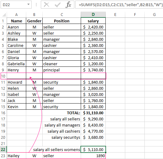
Suppose we need to calculate the amount of salaries of all female sellers for January. We have two conditions. The employee must be:
- a seller;
- a woman.
So, we will use the SUMIFS command.
Enter the arguments.
- Sum range — cells with a salary;
- Criteria range 1 — cells indicating the post of the employee;
- Criteria 1 — the seller;
- Criteria range 2 — cells with gender of the employee;
- Criteria 2 — female (f).
The result: all female sellers in January received in summation 5110$.
SUMIF in Excel with dynamic criterion
The SUMIF and SUMIFS functions are useful because they automatically fit themselves to the changing criteria. That is, we can change the data in cells, and the sums will change with them. For example, when calculating salaries, it turned out that we forgot to take into account one employee who works as a seller. We can add one more line by right-clicking and selecting the ВСТАВИТЬ command.
We have an additional row. We can see that the range of conditions and summations has automatically expanded to 15 rows.
Copy the employee’s data and paste it into the general list. The sums in the resulting cells have changed. The functions have reacted to the appearance of another female seller in the range.
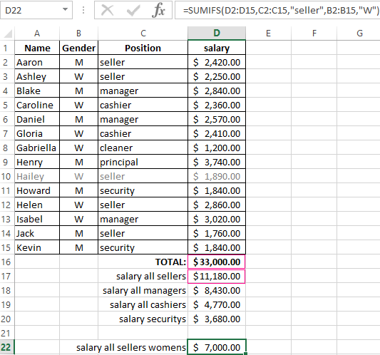
Similarly, you can not only add, but also delete any rows (for example, when the employee is discharged), change the values, etc.
Excel SUMIF Function: Ultimate Guide
In this guide, you are going to learn all about the Excel SUMIF function, which is the most important Excel formula for summarizing your information (and also SUMIFS, which will be tackled later).
Now, the SUMIF is all about conditional summing, that is we only sum all numbers in a range based on one criterion. Aside from numbers, SUMIF can also add cells based on dates and text that match specific criteria. Logical operators can be utilized such as <, >, = and wildcards (*,?) for partial matching.
How to use SUMIF Function
SUMIF function’s syntax is:
=SUMIF(range, criteria, [sum_range])
Range – this is the range of cells that you want to apply the criteria against
Criteria – the criteria used to determine which cells to add
Sum_range – Optional, this is the range of cells to sum together. However, it uses the Range (1st argument) as the sum_range if this parameter is omitted.
Let us explore how to use the Excel SUMIF function:
Suppose we have a list of the quantity of our product (in this case, ribbon) and we want to sum all based on their colors. Below, you can see our data, formulas, and the results returned by our SUMIF formula.
=SUMIF($B$2:$B$11:E2,$C$2:$C$11)
Let’s evaluate our sample starting with the Red ribbons. By manual verification, we can see that we have 2 entries of Red with quantities 16 and 2, which sums up to 18. Next is 3 entries of Blue with quantities 12, 6 and 22. That’s a total of 40. Again, same results returned by the SUMIF formula.
SUMIF Not Equal
SUMIF not equal, by using logical operators “<>” returns the sum of all cells that are NOT EQUAL TO THE SUPPLIED CRITERIA. Here’s a quick example to show how to use it.

Formula in cell F2:
=SUMIF($B$2:$B$11,”<>”&2000,$C$2:$C$11)
Formula in cell F3:
=SUMIF($B$2:$B$11,”<>”&E3,C$2:$C$11)
In our example, we want to get the sum of the persons not born in the year 2000. As you can see, we can use the formula in 2 ways, one is to manually include the criteria (2000) in the formula by typing it in and the other is to use cell reference as shown in the second formula. Both yield the same result (53), but I personally prefer the latter, since it’s dynamic and gives convenience when changing the criteria from one to another.
Another scenario is using text in the ‘not equal to’ criteria. Below is an example:

Formula in cell F2:
=SUMIF($B$2:$B$11,”<>”&”Red”,$C$2:$C$11)
Formula in cell F3:
=SUMIF($B$2:$B$11,”<>”&E3,$C$2:$C$11)
Same as our first example, we can use the formula in 2 ways; 1st is manually typing the text criteria in the formula and the 2nd is to use cell reference. Again, 2nd formula is preferable due to its convenience when changing the criteria from one to another.
Note that the text in criteria is not case sensitive.
SUMIF Date Range
To sum cell values based on dates, you can use SUMIF function together with logical operators <,>, =>, etc. in your criteria. You can refer to the examples below for better comprehension.

Formula in cells F2 and F6:
=SUMIF($B$2:$B$11,”>”&E2,$C$2:$C$11)
=SUMIF($B$2:$B$11,”>”&DATE(2000,5,12),$C$2:$C$11)
Formula in cells F3 and F7:
=SUMIF($B$2:$B$11,”<”&E2,$C$2:$C$11)
=SUMIF($B$2:$B$11,”<”&DATE(2000,5,12),$C$2:$C$11)
Formula in cells F4 and F8:
=SUMIF($B$2:$B$11,”=”&E3,$C$2:$C$11)
=SUMIF($B$2:$B$11,”=”&DATE(2000,5,12),$C$2:$C$11)
Note that ‘=’ operator can be omitted for ‘is equal’ comparison. It will also yield same result.
By looking at the example, there are 2 ways to use the Excel SUMIF function on date ranges. One is by cell referencing and the other is by using the DATE function to create a date.
The DATE function is a safe way to use on function criteria since it creates a valid date from the individual year, month, and day components. This eradicates problems related to regional date settings.
SUMIF Greater Than
To sum cell values that are greater than a given value (criteria), use SUMIF function with “>” at the beginning of criteria argument. You can use it to compare either a number or a text. Here are some examples.

Formula in cell G2:
=SUMIF($C$2:$C$11,”>”&F2,$D$2:$D$11)
Formula in cell G3:
=SUMIF($C$2:$C$11,”>”&F3,$D$2:$D$11)
Formula in cell G4:
=SUMIF($C$2:$C$11,”>”&F4,$D$2:$D$11)
As discussed in the introduction of this article, we can use SUMIF and logical operators to sum cell values that satisfy the comparison criteria, which, in this case, is the greater than ‘>’ operator. Looking at our 1st formula, it sums up all the quantities with prices that are >1,300, and that is the item with product code MD00926 with quantity 35, same as what our formula returned.
SUMIF With Or
Excel SUMIF function is basically designed with AND logic. That means a value must match ALL CONDITIONS for it to be included in the result.
Nevertheless, some techniques allow us to use OR logic instead. One method is to supply Excel SUMIF multiple criteria in an array constant (enclose the criteria list in curly braces ‘{}’) and to wrap the formula in a SUM function like this:
=SUM(SUMIF(range, {“criteria1”, ”criteria2”}, sum_range))
Let’s see an example that is used in a worksheet:

Our sample data consists of 3 variations of a product with different prices and what we want to add up are the ones that are either red or blue. As discussed previously, we can use SUMIF function wrapped inside a SUM function. So, the formula in cell F4 is this:
=SUM(SUMIF($B$2:$B$11,{“Red”,”Blue”},$C$2:$C$11))
Remember that the criteria values should be manually inputted and not as a cell reference. Text values should be enclosed in double quotation marks, and numeric values are without double quotation marks.
Note: This is not an array formula, simply hit Enter key after inputting the formula.
SUMIF Vlookup
If we want to sum the values in a dataset based on matching instances of the specified criteria, we can make a dynamic SUMIF function in Excel by combining it with the VLOOKUP function. The below sample formulas will help you understand how these Excel functions work and how to apply them to actual data.

Suppose our task is to find the total stock quantity of the product Essentials Spring – Super King. Looking at our main table, we only have product codes in our list. Thus, requiring us to search for the product name in the lookup table using its product code.
The first thing that our formula needs to do is to find all the Essentials Spring – Super King mattresses on our Main Table.
The second is to sum all the stock quantity of that product. That means we should enclose the VLOOKUP function inside the SUMIF formula in Excel just like this:
Notice that we used the VLOOKUP as the criteria argument of the Excel SUMIF function. By doing that, we have looked up the product code of Essentials Spring – Super King in our Lookup Table, and then sum up all the stock based on the matched instances of that specific product in our Main Table. Our formula returned a result of 90, equivalent to our manual count of 90 (highlighted in the previous screenshot).
The formula we used in cell B17 is:
=SUMIF($A$3:$A$12,VLOOKUP(B16,$E$3:$F$14,2,0),$C$3:$C$12)
Again, we simply hit Enter key since this is not an array formula.
Excel SUMIF Multiple Criteria
SUMIF Multiple Criteria is Excel SUMIFS
Excel SUMIFS function performs multiple conditions summing, returning the sum of cell values based on multiple criteria.
Or simply, it is the Excel SUMIF multiple criteria or the plural form of SUMIF. However, the Excel SUMIFS function’s syntax is more complex than SUMIF.
=SUMIFS(sum_range, criteria_range1, criteria1, [criteria_range2, criteria2], …)
Note that the first 3 arguments are required, additional ranges and their accompanying criteria are optional.
Just like SUMIF, SUMIFS function is designed to work with AND logic so sum range is added ONLY IF IT MEETS ALL OF THE SPECIFIED CRITERIA.
Tip: You can use up to 127 range & criteria pairs in the Excel SUMIFS formula.
How to Use SUMIFS in Excel
Let’s look at an example data and how SUMIFS function is used.

In this example, we can see that we are looking for the sum using 2 criteria – Product: Orange and Sales Rep.: John.
In order to get the total quantity of oranges John was able to sell, highlight the cell where you want the output to show and use SUMIFS function with formula in cell G3:
=SUMIFS($C$2:$C$13,$B$2:$B$13.$G$2,$A$2:$A$13,$G$2)
By analyzing that, the cells to add are from C2 to C13. Criteria 1 range is from B2 to B13 and criteria 1 is for the cell to have the word “Orange” in it. Criteria 2 range is from A2 to A13 and criteria 2 is for the cell to have the word “John” in it. Thus, the formula adds rows 3, 6 and 11 in column C where it satisfies both conditions.
Note: This is not an array formula, simply hit Enter key after inputting the formula.
SUMIF Multiple Columns
Suppose the data you want to add is in multiple, different columns. There are two scenarios where we may deal with multiple columns. One is if we want to add values of the cells in multiple columns. Here, we can use the Excel SUMIF function by simply doing SUMIF ()+SUMIF()+SUMIF() and so on… Each SUMIF Excel function containing the different sum ranges that need to be added. For instance:

SUMIF
In our example, our purpose is to sum all sales quantity of Watermelon from Monday to Friday. Looking at our formula, we used:
=SUMIF($A$2:$A$13,$A$17,$B$2:$B$13)+SUMIF($A$2:$A$13,$A$17,$C$2:$C$13)+
SUMIF($A$2:$A$13,$A$17,$D$2:$D$13)+SUMIF($A$2:$A$13,$A$17,$E$2:$E$13)+
SUMIF($A$2:$A$13,$A$17,$F$2:$F$13)
Let’s break it down one by one for analysis.
The first SUMIF, SUMIF($A$2:$A$13,$A$17,$B$2:$B$13) refers to: range A2 to A13, criteria Watermelon in cell A17, and with sum range in column B – Monday. That means we will sum all quantities of Watermelon sales on Monday. Now, to add the all the watermelon sales on Tuesday, we will add another SUMIF function, replacing the sum range to column C like so. SUMIF($A$2:$A$13,$A$17,$C$2:$C$13). And so on, until we have included all watermelon sales across column F which is Friday.
The second scenario is where we may need to sum up values across multiple columns with multiple criteria. The solution is to combine SUMIF function with INDEX and MATCH functions. This will be the syntax:
=SUMIF(range, criteria, INDEX(array, , MATCH(lookup_value,lookup_array,[match_type])))
Let us try to use that in an Excel worksheet.

In this example, we want to add all Watermelon sales on Wednesday. Looking at our formula we can see that we have replaced the sum_range argument with INDEX & MATCH functions. This way, we are horizontally searching for our second criteria which is Wednesday across multiple columns. And so, we have a result of 35. Manually counting, we also get the value of 35.
Note: This is not an array formula, simply hit Enter key after inputting the formula.
SUMPRODUCT for Dealing With Excel SUMIF Multiple Criteria
In case our multiple criteria are listed in the worksheet instead of manually inputted in the formula, we can use SUMIF and SUMPRODUCT functions together. The SUMPRODUCT function multiplies the components in the given arrays and returns the sum of the items. Below is a sample formula used in the worksheet:

Formula used in cell B19:
=SUMPRODUCT(SUMIF($A$2:$A$13,$A$17:$A$18,$B$2:$B$13))
Alternatively, you can still list the criteria directly into the formula enclosed in curly braces like so:
=SUMPRODUCT(SUMIF($A$2:$A$13{“Watermelon”, “Apple”},$B$2:$B$13))
Both methods will be returning same results.
Note: This is not an array formula, simply hit Enter key after inputting the formula.
Troubleshooting
Array Arguments to SUMIFS are of Different Size
When using SUMIFS function always make sure that the sum range and all criteria ranges are the same size and orientation. In other words, if the sum range column is in a column from row 1 to 100, then the criteria range MUST be in a column with the same number of rows as well.
Look at the illustrations below:

See that #VALUE! error? Look at the picture below with highlighted formula arguments. Notice that the first argument range is from row 2 to 11, but the sum_range is from row 3 to 11.

Let’s evaluate the formula:
=SUMIFS($C$3:$C$11,$B$2:$B$11,”>=”&B13,$B$2:$B$11,”<=”&B14)
$C$3:$C$11 – sum_range (row 3 to 11)
$B$2:$B$11 – criteria_range1 (row 2 to 11)
This is what caused the #VALUE! error in cell B16.
Again, always keep in mind when using SUMIFS: The sum_range and criteria ranges are required to be same in size and orientation.
The SUMIF Excel function calculates the sum of a range of cells based on given criteria. The criteria can include dates, numbers, and text. For example, the formula “=SUMIF(B1:B5, “<=12”)” adds the values in the cell range B1:B5, which are less than or equal to 12.
SUMIF function is categorized under the Excel Math and Trigonometry functions. Moreover, this function works similar to the SUMIFS functionSUMIFS is an enhanced version of the SUMIF formula in Excel that enables you to sum any range of data by matching several criteria. read more. The SUMIF function uses a single criterion, whereas the SUMIFS function uses multiple criteria.
Table of contents
- SUMIF in Excel
- SUMIF Formula in Excel
- How to Use the SUMIF Excel Function?
- Example #1
- Example #2
- Example #3
- Example #4
- The “Criteria” Argument of the SUMIF Function
- Frequently Asked Questions (FAQs)
- SUMIF Excel Function Video
- Recommended Articles
SUMIF Formula in Excel
The SUMIF formula is stated as follows:

The formula accepts the following arguments:
- Range: It refers to the range of cells on which the criteria is applied.
- Criteria: It refers to the conditions that are applied to the range of cells. It determines the cells to be added from the given “sum_range.”
- Sum_range: It indicates the range of cells to be added together.
“Range” and “criteria” are the required parameters, whereas “sum_range” is an optional parameter.
Note: If “sum_range” is not specified, the SUMIF function refers to the parameter “range” as the range of cells to be added.
How to Use the SUMIF Excel Function?
Let us understand the SUMIF excel function with the help of the following examples. Each example covers a different case, implemented using the SUMIF function.
You can download this SUMIF Function in Excel Template here – SUMIF Function in Excel Template
Example #1
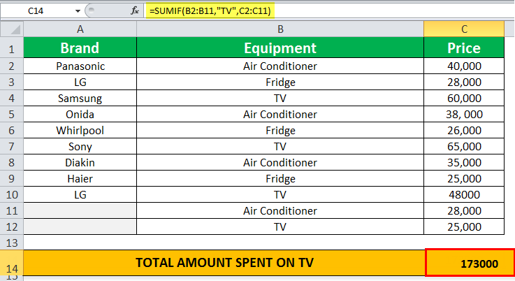
Total Amount Spent on Branded Televisions (TVs)
The following table shows a list of branded equipment and their prices. For some equipment, the brands are not specified. We have to calculate the total amount spent on purchasing branded TVs using the SUMIF function.
In the succeeding table, the cells that satisfy the given criteria are C4, C7, and C10, which shows the prices of the branded TVs. Hence, the sum of the values of cells C4, C7, and C10 is 1,73,000, shown in cell C14. This is the total amount spent on purchasing branded TVs.
The following SUMIF formula is applied to the range C2:C11:
“=SUMIF(B2:B11,“TV”,C2:C11)”
Where,
- B2:B11 refers to the range of cells on which the specific criterion is to be applied.
- “TV” refers to the condition applied to the range B2:B11.
- C2:C11 refers to the range of values to be added.
Example #2
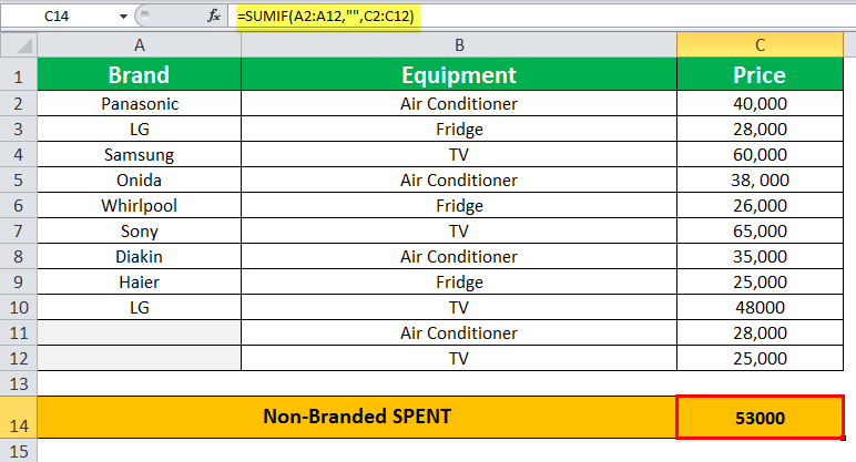
Sum of the Amount Spent on Non-Branded Items
Working on the data of example #1, we want to calculate the total amount spent on purchasing non-branded items using the SUMIF function.
In the following table, the cells C11 and C12 satisfy the given criteria where no brand name is entered in the cells. Hence, the sum of the values of cells C11and C12 is 53,000, as shown in cell C14. This indicates the total amount spent on purchasing non-branded items.
The following SUMIF formula is applied to the range C2:C12:
“=SUMIF(A2:A12,“”,C2:C12)”
Where,
- A2:A12 refers to the range of cells on which the specific criterion is to be applied.
- “” refers to the condition which checks for blank cells in the range B2:B12.
- C2:C12 is the range of values to be summed up.
Example #3
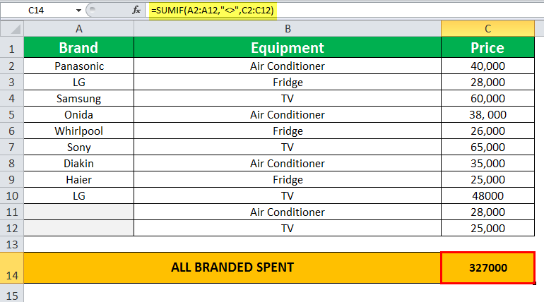
Sum of the Amount Spent on Branded Items
Working on the data of example #1, we want to calculate the total amount spent on branded items using the SUMIF function.
In the following table, the cells B11, B12 satisfy the given criteria with no brand names. Hence, the sum of the values of C1 to C10 is 53,000, displayed in cell C14. This is the total amount spent on purchasing branded items. The cells C11 and C12 are skipped because they are blank cells.
The following SUMIF formula is applied to the range C2:C12:
“=SUMIF(A2:A12,“<>”,C2:C12)”
Where,
- A2:A12 refers to the range on which the criteria are to be applied.
- “<>” is the condition which checks for non-blank cells in the range B2:B12.
- C2:C12 is the range of values to be added.
Example #4
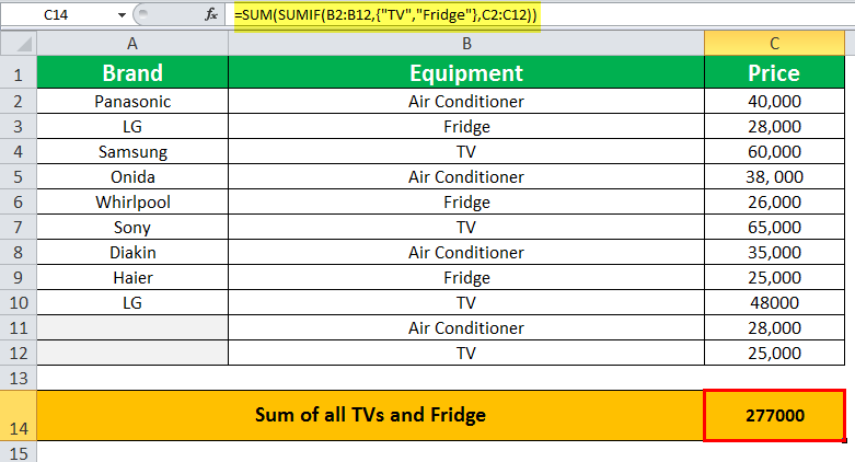
Sum of the Two Different Items
Working on the data of example #1, we want to calculate the sum of two different items using the SUMIF formula.
The following table shows the total amount calculated by adding the sum of the prices of two items – TV and fridge in the cell C14, using the SUMIF formula. The SUM of the prices of the fridges and TVs are 79,000 and 1,98,000, respectively. Hence, the total SUM of the prices of two items is 2,77,000.
The SUMIF formula is applied to the range C2:C12 and is stated as follows:
“=SUM(SUMIF(B2:B12,{“TV”,“Fridge”},C2:C12))”
Where,
- B2: B12 refers to the range on which the criteria are to be applied.
- “TV,” “fridge” refers to the two individual conditions to be checked in range B2: B12. The curly braces {} of the criterion represent the collection of constants.
- C2: C12 refers to the range of values to be added.
In the formula, the SUMIF function is enclosed within the SUM function. The SUMIF formula executes two different conditions, “TV” and “fridge.” Finally, the SUM functionThe SUM function in excel adds the numerical values in a range of cells. Being categorized under the Math and Trigonometry function, it is entered by typing “=SUM” followed by the values to be summed. The values supplied to the function can be numbers, cell references or ranges.read more sums the results of the SUMIF functions to return the output.
The “Criteria” Argument of the SUMIF Function
The guidelines of the argument of the SUMIF formula are stated as follows:
- The numeric criteria are not enclosed in double quotes.
- The text criteria for SUMIFSUMIF function is a conditional IF function to sum the cells based on specific criteria. For example, to add a group of cells, if the cell adjacent to them has a specified text in them, then function is used as follows =SUMIF(Text Range,” Text”, cells range for sum).read more, including the mathematical symbols, are enclosed within double quotes.
- The wildcard characters – question mark (?) and asterisk (*) used in the criteria match a single character and a series of characters, respectively.
- The tilde operator (~) followed by the wildcard characters refer to the actual characters. For example, the “~?” indicates criteria as a question mark literally.
- The SUMIF formula returns “#VALUE! error” when the criterion is a text string that is greater than 255 characters.
Frequently Asked Questions (FAQs)
1. What is the SUMIF function in Excel?
The SUMIF function returns the sum of cells that satisfy the given criteria. This worksheet (WS) function is categorized as a Math and Trigonometry function. Furthermore, for partial matching, it uses logical operators and wildcards.
The SUMIF formula is stated as follows:
“=SUMIF(range, criteria, [sum_range])”
Where,
• Range refers to the range of cells against which we need to apply the criteria.
• Criteria are the conditions that are applied to the range of cells.
• Sum_range is an array of numeric values. The values are added if the specific criterion matches the range.
The “range” and “criteria” are the required arguments, and “sum_range” is an optional argument.
Note: If the argument “sum_range” is omitted, the values in the “range” will be added.
2. How to use the SUMIF Excel function for multiple criteria?
The formula for the SUMIF with multiple criteria is stated as follows:
“=SUMIF(sum_range, range 1, criteria1)+SUMIF(sum_range, range 2, criteria2)”
Where,
• Sum_range refers to the range of cells to be added.
• Range1, range 2 are the range of cells on which the criteria are to be applied.
• Criteria1, criteria 2 are the conditions applied to the respective range of cells. Alternatively, we can use the SUMIFS function to sum cells satisfying the multiple criteria.
3. Can we use the SUMIF function with text criteria?
The SUMIF excel function can be used to add cells containing text strings that meet specific criteria. In the formula, the text criteria are enclosed in double quotes.
For example, consider the below SUMIF formula:
“=SUMIF(A1:A4,“Purple”,B1:B4)”
The formula adds the values in range B1:B4 if the range A1:A4 contains the text “Purple”.
SUMIF Excel Function Video
Recommended Articles
This has been a guide to SUMIF Excel Function. Here we discuss how to use SUMIF Formula along with excel examples and downloadable templates. You may also look at these useful functions in Excel –
- Excel SUM ShortcutThe Excel SUM Shortcut is a function that is used to add up multiple values by simultaneously pressing the “Alt” and “=” buttons in the desired cell. However, the data must be present in a continuous range for this function to function.read more
- SUMIF With VLOOKUPSUMIF is used to sum cells based on some condition, which takes arguments of range, criteria, or condition, and cells to sum. When there is a large amount of data available in multiple columns, we can use VLOOKUP as the criteria.read more
- Excel SUMIF Between Two DatesWhen we wish to work with data that has serial numbers with different dates and the condition to sum the values is based between two dates, we use Sumif between two dates. read more
- SUM in ExcelThe SUM function in excel adds the numerical values in a range of cells. Being categorized under the Math and Trigonometry function, it is entered by typing “=SUM” followed by the values to be summed. The values supplied to the function can be numbers, cell references or ranges.read more