
Excel for Microsoft 365 Excel 2021 Excel 2019 Excel 2016 Excel 2013 Excel 2010 More…Less
Just by using the Power Query Editor, you have been creating Power Query formulas all along. Let’s see how Power Query works by looking under the hood. You can learn how to update or add formulas just by watching the Power Query Editor in action. You can even roll your own formulas with the Advanced Editor.
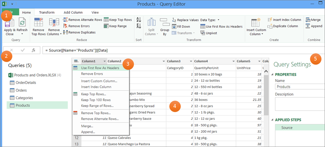
The Power Query Editor provides a data query and shaping experience for Excel that you can use to reshape data from many data sources. To display the Power Query Editor window, import data from external data sources in an Excel worksheet, select a cell in the data, and then select Query > Edit. The following is a summary of the main components.
-
The Power Query Editor ribbon that you use to shape your data
-
The Queries pane that you use to locate data sources and tables
-
Context menus that are convenient shortcuts to commands in the ribbon
-
The Data Preview that displays the results of the steps applied to the data
-
The Query Settings pane that lists properties and each step in the query
Behind the scenes, each step in a query is based on a formula that is visible in the formula bar.
There may be times when you want to modify or create a formula. Formulas use the Power Query Formula Language, which you can use to build both simple and complex expressions. For more information about syntax, arguments, remarks, functions, and examples, see Power Query M formula language.
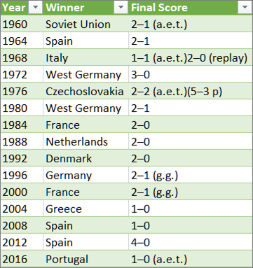
Using a list of soccer championships as an example, use Power Query to take raw data that you found on a website and turn it into a well-formatted table. Watch how query steps and corresponding formulas are created for each task in the Query Settings pane under Applied Steps and in the Formula bar.

Procedure
-
To import the data, select Data > From Web, enter «http://en.wikipedia.org/wiki/UEFA_European_Football_Championship» in the URL box, and then select OK.
-
In the Navigator dialog box, select the Results [Edit] table on the left, and then select Transform Data at the bottom. The Power Query editor appears.
-
To change the default query name, in the Query Settings pane, under Properties, delete «Results [Edit]» and then enter «UEFA champs».
-
To remove unwanted columns, select the first, fourth, and fifth columns, and then select Home > Remove Column > Remove Other Columns.
-
To remove unwanted values, select Column1, select Home > Replace Values, enter «details» in the Values to Find box, and then select OK.
-
To remove rows that have the word «Year’ in them, select the filter arrow in Column1, clear the check box next to «Year», and then select OK.
-
To rename the column headers, double-click each of them and then change «Column1» to «Year», «Column4» to «Winner», and «Column5» to «Final Score».
-
To save the query, select Home > Close & Load.
Result
The following table is a summary of each applied step and the corresponding formula.
|
Query step and task |
Formula |
|---|---|
|
Source Connect to a web data source |
= Web.Page(Web.Contents(«http://en.wikipedia.org/wiki/UEFA_European_Football_Championship»)) |
|
Navigation Select the table to connect |
=Source{2}[Data] |
|
Changed Type Change datatypes (which Power Query does automatically) |
= Table.TransformColumnTypes(Data2,{{«Column1», type text}, {«Column2», type text}, {«Column3», type text}, {«Column4», type text}, {«Column5», type text}, {«Column6», type text}, {«Column7», type text}, {«Column8», type text}, {«Column9», type text}, {«Column10», type text}, {«Column11», type text}, {«Column12», type text}}) |
|
Removed Other Columns Remove other columns to only display columns of interest |
= Table.SelectColumns(#»Changed Type»,{«Column1», «Column4», «Column5»}) |
|
Replaced Value Replace values to clean up values in a selected column |
= Table.ReplaceValue(#»Removed Other Columns»,»Details»,»»,Replacer.ReplaceText,{«Column1»}) |
|
Filtered Rows Filter values in a column |
= Table.SelectRows(#»Replaced Value», each ([Column1] <> «Year»)) |
|
Renamed Columns Changed column headers to be meaningful |
= Table.RenameColumns(#»Filtered Rows»,{{«Column1», «Year»}, {«Column4», «Winner»}, {«Column5», «Final Score»}}) |
Important Be careful editing the Source, Navigation, and Changed Type steps because they are created by Power Query to define and set up the data source.
Show or hide the formula bar
The formula bar is shown by default, but if it’s not visible you can redisplay it.
-
Select View > Layout > Formula Bar.
Edit a formula in the formula bar
-
To open a query, locate one previously loaded from the Power Query Editor, select a cell in the data, and then select Query > Edit. For more information see Create, load, or edit a query in Excel.
-
In the Query Settings pane, under Applied Steps, select the step you want to edit.
-
In the formula bar, locate and change the parameter values, and then select the Enter
 icon or press Enter. For example, change this formula to also keep Column2:
Before: = Table.SelectColumns(#»Changed Type»,{«Column4», «Column1», «Column5»})
After:= Table.SelectColumns(#»Changed Type»,{«Column2», «Column4», «Column1», «Column5»}) -
Select the Enter
icon or press Enter to see the new results displayed in the Data Preview. -
To see the result in an Excel worksheet, select Home > Close & Load.
 icon or press Enter. For example, change this formula to also keep Column2:
Create a formula in the formula bar
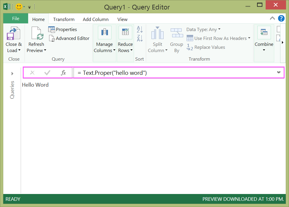
For a simple formula example, let’s convert a text value to proper case using the Text.Proper function.
-
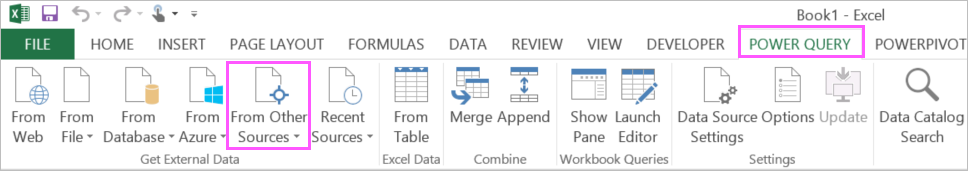
To open a blank query, in Excel select Data > Get Data > From Other Sources > Blank Query. For more information see Create, load, or edit a query in Excel.
-
In the formula bar, enter =Text.Proper(«text value»), and then select the Enter
icon or press Enter.The results display in Data Preview .
-
To see the result in an Excel worksheet, select Home > Close & Load.
Result:
When you create a formula, Power Query validates the formula syntax. However, when you insert, reorder, or delete an intermediate step in a query you might potentially break a query. Always verify the results in Data Preview.
Important Be careful editing the Source, Navigation, and Changed Type steps because they are created by Power Query to define and set up the data source.
Edit a formula by using a dialog box
This method makes use of dialog boxes that vary depending on the step. You don’t need to know the syntax of the formula.
-
To open a query, locate one previously loaded from the Power Query Editor, select a cell in the data, and then select Query > Edit. For more information see Create, load, or edit a query in Excel.
-
In the Query Settings pane, under Applied Steps, select the Edit Settings
icon of the step you want to edit or right-click the step, and then select Edit Settings. -
In the dialog box, make your changes, and then select OK.
 icon of the step you want to edit or right-click the step, and then select Edit Settings.
Insert a step
After you complete a query step that reshapes your data, a query step is added below the current query step. but when you insert a query step in the middle of the steps, an error might occur in subsequent steps. Power Query displays an Insert Step warning when you try to insert a new step and the new step alters fields, such as column names, that are used in any of the steps that follow the inserted step.
-
In the Query Settings pane, under Applied Steps, select the step you want to immediately precede the new step and its corresponding formula.
-
Select the Add Step
icon to the left of the formula bar. Alternatively, right click a step and then select Insert Step After. A new formula is created in the format := <nameOfTheStepToReference>, such as =Production.WorkOrder.
-
Type in the new formula using the format:
=Class.Function(ReferenceStep[,otherparameters])
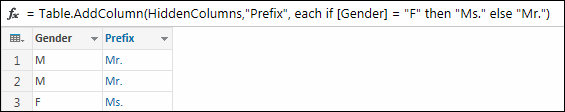
For example, assume you have a table with the column Gender and you want to add a column with the value “Ms.” or “Mr.”, depending on the person’s gender. The formula would be:
=Table.AddColumn(<ReferencedStep>, «Prefix», each if [Gender] = «F» then «Ms.» else «Mr.»)
 icon to the left of the formula bar. Alternatively, right click a step and then select Insert Step After. A new formula is created in the format :
Reorder a step
-
In the Queries Settings pane under Applied Steps, right click the step, and then select Move Up or Move Down.
Delete a step
-
Select the Delete
icon to the left of the step, or right click the step, and then select Delete or Delete Until End. The Delete icon is also available to the left of the formula bar.
 icon to the left of the step, or right click the step, and then select Delete or Delete Until End. The Delete
 In this example, let’s convert the text in a column to proper case using a combination of formulas in the Advanced Editor.
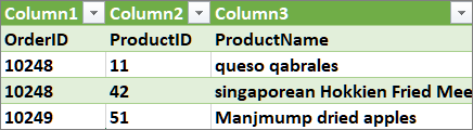
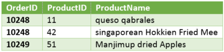
For example, you have an Excel table, called Orders, with a ProductName column that you want to convert to proper case.
Before:
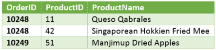
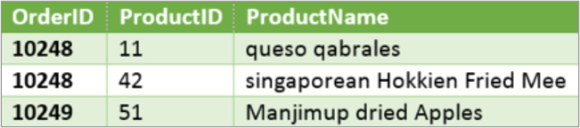
After:
When you create an advanced query, you create a series of query formula steps based on the let expression. Use the let expression to assign names and calculate values that are then referenced by the in clause, which defines the Step. This example returns the same result as the one in the «Create a formula in the formula bar» section.
let
Source = Text.Proper(«hello world»)
in
Source
You’ll see that each step builds upon a previous step by referring to a step by name. As a reminder, the Power Query Formula Language is case-sensitive.
Phase 1: Open the Advanced Editor
-
In Excel, select Data > Get Data > Other Sources > Blank Query. For more information see Create, load, or edit a query in Excel.
-
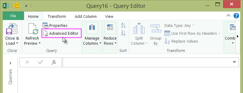
In the Power Query Editor, select Home > Advanced Editor, which opens with a template of the let expression.

Phase 2: Define the data source
-
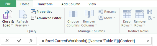
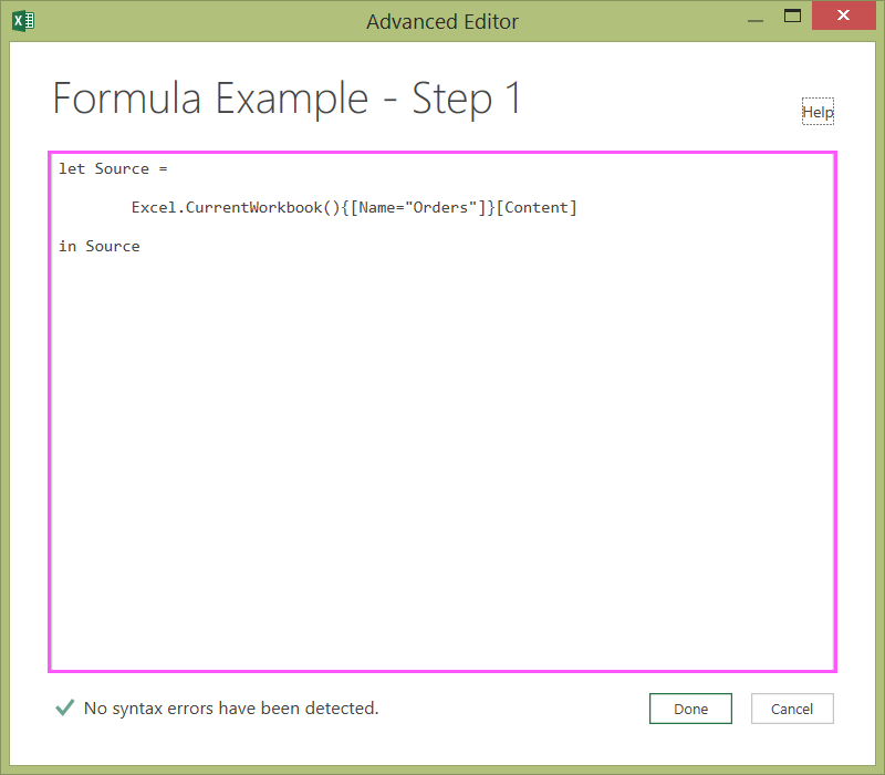
Create the let expression using the Excel.CurrentWorkbook function as follows:
let
Source = Excel.CurrentWorkbook(){[Name=»Orders»]}[Content]
in
Source -
To load the query to a worksheet, select Done, and then select Home > Close & Load > Close & Load.
Result:
Phase 3: Promote the first row to headers
-
To open the query, from the worksheet select a cell in the data, and then select Query > Edit. For more information see Create, load, or edit a query in Excel (Power Query).
-
In the Power Query Editor, select Home > Advanced Editor, which opens with the statement you created in Phase 2: Define the data source.
-
In the let expression, add #»First Row as Header» and Table.PromoteHeaders function as follows:
let
Source = Excel.CurrentWorkbook(){[Name=»Orders»]}[Content],
#»First Row as Header» = Table.PromoteHeaders(Source)
in
#»First Row as Header» -
To load the query to a worksheet, select Done, and then select Home > Close & Load > Close & Load.
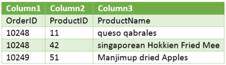
Result:
Phase 4: Change each value in a column to proper case
-
To open the query, from the worksheet select a cell in the data, and then select Query > Edit. For more information see Create, load, or edit a query in Excel.
-
In the Power Query Editor, select Home > Advanced Editor, which opens with the statement you created in Phase 3: Promote the first row to headers.
-
In the let expression, convert each ProductName column value to proper text by using the Table.TransformColumns function, referring to the previous «First Row as Header” query formula step, adding #»Capitalized Each Word» to the data source, and then assigning #»Capitalized Each Word» to the in result.
let
Source = Excel.CurrentWorkbook(){[Name=»Orders»]}[Content],
#»First Row as Header» = Table.PromoteHeaders(Source),
#»Capitalized Each Word» = Table.TransformColumns(#»First Row as Header»,{{«ProductName», Text.Proper}})
in
#»Capitalized Each Word» -
To load the query to a worksheet, select Done, and then select Home > Close & Load > Close & Load.
Result:
You can control the behavior of the formula bar in the Power Query Editor for all your workbooks.
Display or hide the formula bar
-
Select File > Options and Settings > Query Options.
-
In the left pane, under GLOBAL, select Power Query Editor.
-
In the right pane, under Layout, select or clear Display the Formula Bar.
Turn on or off M Intellisense
-
Select File > Options and Settings > Query Options .
-
In the left pane, under GLOBAL, select Power Query Editor.
-
In the right pane, under Formula, select or clear Enable M Intellisense in the formula bar, advanced editor, and custom column dialog.
Note Changing this setting will take effect the next time you open the Power Query Editor window.
See Also
Power Query for Excel Help
Create and invoke a custom function
Using the Applied Steps list (docs.com)
Using custom functions (docs.com)
Power Query M formulas (docs.com)
Dealing with errors (docs.com)
Need more help?
Want more options?
Explore subscription benefits, browse training courses, learn how to secure your device, and more.
Communities help you ask and answer questions, give feedback, and hear from experts with rich knowledge.
Excel for Microsoft 365 Excel 2021 Excel 2019 Excel 2016 Excel 2013 Excel 2010 More…Less
Note: This article has done its job, and will be retiring soon. To prevent «Page not found» woes, we’re removing links we know about. If you’ve created links to this page, please remove them, and together we’ll keep the web connected.
Note:
Power Query is known as Get & Transform in Excel 2016. Information provided here applies to both. To learn more, see Get & Transform in Excel 2016.
To create Power Query formulas in Excel, you can use the Query Editor formula bar, or the Advanced Editor. The Query Editor is a tool included with Power Query that lets you create data queries and formulas in Power Query. The language used to create those formulas is the Power Query Formula Language. There are many Power Query formulas you can use to discover, combine and refine data. To learn more about the full range of Power Query formulas, see Power Query formula categories.
Let’s create a simple formula, and then create an advanced formula.
-
Create a simple formula
-
Create an advanced formula
Create a simple formula
For a simple formula example, let’s convert a text value to proper case using the Text.Proper() formula.
-
In the POWER QUERY ribbon tab, choose From Other Sources > Blank Query.
-
In the Query Editor formula bar, type = Text.Proper(«text value»), and press Enter or choose the Enter icon.
-
Power Query shows you the results in the formula results pane.
-
To see the result in an Excel worksheet, choose Close & Load.
The result will look like this in a worksheet:
You can also create advanced query formulas in the Query Editor.
Create an advanced formula
For an advanced formula example, let’s convert the text in a column to proper case using a combination of formulas. You can use the Power Query Formula Language to combine multiple formulas into query steps that have a data set result. The result can be imported into an Excel worksheet.
Note: This topic is an introduction to advanced Power Query formulas. To learn more about Power Query formulas, see Learn about Power Query formulas.
For example, let’s assume you have an Excel table with product names you want to convert to proper case.
The original table looks like this:
And, you want the resulting table to look like this:
Let’s go through the query formula steps to change the original table so that the values in the ProductName column are proper case.
Advanced query using Advanced Editor example
To clean up the original table, you use the Advanced Editor to create query formula steps. Let’s build each query formula step to show how to create an advanced query. The complete query formula steps are listed below. When you create an advanced query, you follow this process:
-
Create a series of query formula steps that start with the let statement. Please note that the Power Query Formula Language is case sensitive.
-
Each query formula step builds upon a previous step by referring to a step by name.
-
Output a query formula step using the in statement. Generally, the last query step is used as the in final data set result.
Step 1 – Open Advanced Editor
-
In the POWER QUERY ribbon tab, choose From Other Sources > Blank Query.
-
In Query Editor, choose Advanced Editor.
-
You will see the Advanced Editor.
Step 2 – Define the original source
In the Advanced Editor:
-
Use a let statement that assigns Source = Excel.CurrentWorkbook() formula. This will use an Excel table as the data source. For more information about the Excel.CurrentWorkbook() formula, see Excel.CurrentWorkbook.
-
Assign Source to the in result.
let Source = Excel.CurrentWorkbook(){[Name="Orders"]}[Content] in Source -
Your advanced query will look like this in the Advanced Editor.
-
To see the results in a worksheet:
-
Click Done.
-
In the Query Editor ribbon, click Close & Load.
-
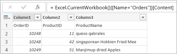
The result looks like this in a worksheet:
Step 3 – Promote the first row to headers
To convert the values in the ProductName column to proper text, you first need to promote the first row to become the column headers. You do this in the Advanced Editor:
-
Add a #»First Row as Header» = Table.PromoteHeaders() formula to your query formula steps and refer to Source as the data source. For more information about the Table.PromoteHeaders() formula, see Table.PromoteHeaders.
-
Assign #»First Row as Header» to the in result.
let
    Source = Excel.CurrentWorkbook(){[Name="Orders"]}[Content],
    #"First Row as Header" = Table.PromoteHeaders(Source)
in
    #"First Row as Header"
The result looks like this in a worksheet:
Step 4 – Change each value in a column to proper case
To convert each ProductName column value to proper text, you use Table.TransformColumns() and refer to the «First Row as Header” query formula step. You do this in the Advanced Editor:
-
Add a #»Capitalized Each Word» = Table.TransformColumns() formula to your query formula steps and refer to #»First Row as Header» as the data source. For more information about the Table.TransformColumns() formula, see Table.TransformColumns.
-
Assign #»Capitalized Each Word» to the in result.
let
    Source = Excel.CurrentWorkbook(){[Name="Orders"]}[Content],
    #"First Row as Header" = Table.PromoteHeaders(Source),
    #"Capitalized Each Word" = Table.TransformColumns(#"First Row as Header",{{"ProductName", Text.Proper}})
in
    #"Capitalized Each Word"
The final result will change each value in the ProductName column to proper case, and looks like this in a worksheet:
With the Power Query Formula Language you can create simple to advanced data queries to discover, combine and refine data. To learn more about Power Query, see Microsoft Power Query for Excel Help.
Need more help?
Formulas are the lifeblood of Excel; they are essential to achieve even basic tasks. On the other hand, Power Query has been designed so that most transformations are accessed through the intuitive user interface. But Power Query formulas exist; it has a formula language with over 700 functions.
Each time we make a transformation with the user interface, Power Query formulas are used in the background. We can see them in the Formula Bar and Advanced Editor.
Do we need to use Power Query formulas?
When I started using Power Query, I used lots of formulas because that is what I did in Excel. However, once I understood the interface, it became clear that many transformations can be achieved without manually writing any formulas. Therefore, I recommend you look for transformations available from the standard menus before delving into specific functions.
Formulas are essential to tackle some of the more complicated situations we might encounter. So, you can’t avoid them entirely.
One confusion is that the functions are not the same as Excel’s; they are written using M code. At the start, it’s frustrating that we can’t transfer our existing Excel knowledge into Power Query. But once we understand how the formulas are constructed, it is easy to find what you need.
Where can we write Power Query formulas?
Every transformation we undertake in Power Query is a formula. When we promote headers, it creates a formula:
= Table.PromoteHeaders(#"Changed Type", [PromoteAllScalars=true])Or if we split a column by a comma, Power Query writes a formula
= Table.SplitColumn(#"Changed Type", "Text", Splitter.SplitTextByDelimiter(",", QuoteStyle.Csv), {"Text.1", "Text.2"})We can write these formulas directly into the Formula Bar or the Advanced Editor. Though, if you are getting started, these can be overwhelming. The most accessible place to start is the Custom Column dialog box.
When we use a Custom Column, it is writing a formula inside the Table.AddColumn function. Even if we just enter 1+1 as a formula. Power Query wraps this in the Table.AddColumn transformation.
= Table.AddColumn(Source, "New Column Name", each 1+1)As this post is part of an introductory series into Power Query, we will focus on writing formulas inside a custom column. But be aware that much more is possible if you want to go further.
Writing a Power Query formula in a Custom Column
The easiest place to write a Power Query formula is in a custom column.
Create a custom column by clicking Add Column > Custom Column.
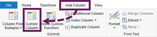
The Custom Column dialog box opens.
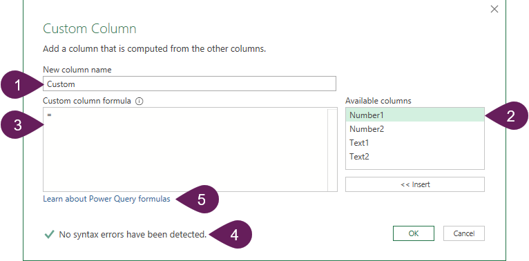
The critical areas of this dialog box are:
- New column name
The text entered here is used as the column name in the table. - Available columns
This contains a list of columns in the query which exist in the previous step. Selecting a column and clicking the Insert button (or double-clicking the name) inserts the column name into the formula. This is useful as it reduces typos that stop our code from working as intended. - Custom column formula
This is where we enter the text which forms the formula. - Error check
The error check helps to let us know if the syntax is correct. For example, it will check if matching opening and closing brackets exist. However, it will not tell us if the formula gives the right result, only that the syntax is correct. Actually, it’s challenging to interpret what the errors mean. To learn more about the types of errors we might encounter, check out this post: Power Query – Common Errors & How to Fix Them. - Learn about Power Query formulas
This link takes us to Microsoft’s Power Query formulas web pages. If you get stuck, this is the place to go.
Simple formula operations
Simple formula operations are similar to Excel.
We do not need to enter the equals symbol ( = ) at the start; it will automatically be in the formula box.
Numeric operators
=[Column 1] + [Column 2] //Addition
=[Column 1] - [Column 2] //Subtraction
=[Column 1] * [Column 2] //Multiplication
=[Column 1] / [Column 2] //Division
=[Column 1] & [Column 2] //Concatenate
Brackets / Parentheses
Parentheses or Brackets (depending on what you call them) work the same as in Excel.
=([Column 1] + [Column 2]) / [Column 3]Logical operators
=[Column 1] = [Column 2] //Equal
=[Column 1] > [Column 2] //Greater Than
=[Column 1] >= [Column 2] //Greater Than or Equal To
=[Column 1] < [Column 2] //Less Than
=[Column 1] <= [Column 2] //Less Than or Equal To
=[Column 1] <> [Column 2] //Does Not Equal
The formulas above will give a True or False result.
Power
The Power operator ( ^ ) we use in Excel does not work in Power Query formulas. Instead, we have to use the Number.Power formula.
Formula Example #1
The screenshot below shows some basic formula operations in action.
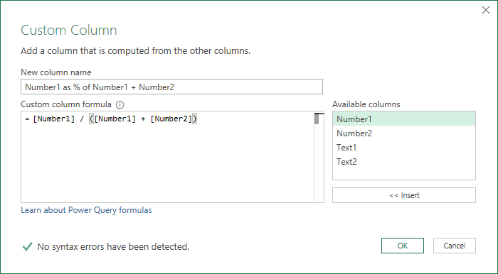
You can see the column names being used; Number1 is divided by the total of Number1 + Number2.
Formula Example #2
The screenshot below shows that formulas can be constructed from static values.
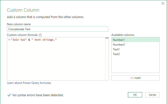
A formula can include a mix of columns and static values.
Row Context
Unless you do some advanced formula magic, the formulas in Power Query have what is known as Row Context. This means the formula is applied to each row one by one.
Data types
Power Query formulas are picky about data types.
If the column used within the function is not the correct data type, the formula will calculate an error. So, if the data type does not match the formula requirements, we need to find a way to convert it. We can either add a step before creating the custom column or use a converting formula.
Some of the most common converting formulas are:
- Text.From – To convert anything to text
- Date.ToText – To convert a date to text
- Date.From – To convert a number into a date
- Date.FromText – To convert text into a date
- Number.ToText – To convert a number to text
- Number.From – To convert any inputs to a number
- Number.FromText – To convert text into a number
- Logical.From – To convert numbers into their True or False values
- Logical.FromText – To convert text strings of “True” or “False” into boolean values of True or False
- Logical.ToText – To convert Boolean True or False values into “True” or “False” text strings
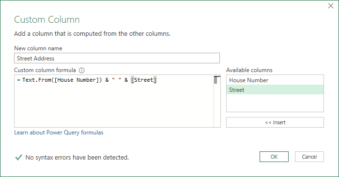
Formula Example #3
The following table contains numbers and text. As the House Number is numeric, we need to convert it to text before combining it with Street Name into a single address string.

The formula text would be:
=Text.From([House Number]) & " " & [Street]The bold text highlights the use of the Text.From function to convert the House Number into a Text data type before combining with the Street Name column.
Finding Functions
As noted earlier, we cannot use Excel formulas inside Power Query.
Power Query function library
The easiest way to find the available formulas is to click the Learn about Power Query formulas link.
The functions are grouped by what they do. We will look at the Number group if we want a formula that uses or returns numbers. Most of the formulas in this section start with the word Number. Here are some examples:
- Number.Abs – Returns the absolute value of a number
- Number.FromText – Returns a number from a text string
- Number.IsOdd – Returns true if the value is odd, or false if it is even.
Specific number formulas might start with other words too, such as:
- Decimal.From – Returns a decimal from a given value
- Percentage.From – Returns a percentage from a given value
Generally, formulas that output a date start with Date in the formula name (such as Date.Year), and formulas that output text start with Text in the formula name (such as Text.Start).
Think about Excel functions; how did you learn them? You probably had someone show you, or you had to do some guesswork with a lot of trial and error. Because of how Power Query functions are named, it is much easier to find the function we want.
#Shared to show Power Query functions
Another option to discover the Power Query function is entering #shared in the formula bar.
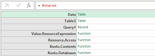
This provides us with a complete list of functions. We can click on any function name to find out about it.
IntelliSense
Power Query has IntelliSense built in. This means we can start typing the name of a function, and a list of options appears. For example, the screenshot below shows the list of functions just by typing “Tex” into the formula box.
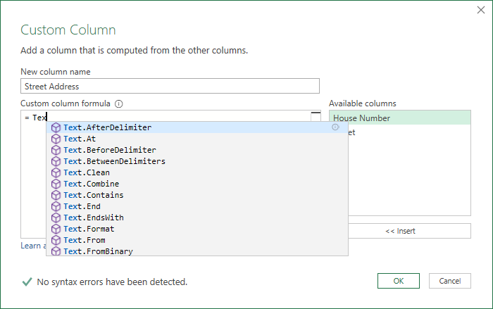
Note: At the time of writing, an annoying bug makes IntelliSense repeat words when formulas are entered. Check out this video for further details on how to avoid it: https://www.youtube.com/watch?v=p3hhUZwQGVE
IntelliSense helps us to discover functions and makes them easier to use. After you’ve got the name of the function, type the opening bracket, and Power Query shows the arguments and data types required. It took a while for Power Query to get this functionality, but now that it’s here, I couldn’t live without it.
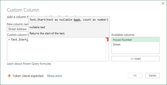
In the screenshot above, we can see that Text.Start has text as the first argument, which must be a text data type.
Looking at existing transformation steps
The transformations we use through the standard interface use functions. Therefore, we can use these as a guide to help us write our own formulas.
Let’s say we wanted to extract the first 4 letters from a text string. We could use Add Column > Extract > First Characters from the Ribbon, then insert 4 into the Insert First Character dialog box. Then, we could take a look at the M code in the Formula Bar for that applied step; it would show the following:
= Table.AddColumn(#"Changed Type", "First Characters", each Text.Start([Text Column], 4), type text)The bold section is the function Text.Start. This function extracts the first characters from a text string (it is similar to Excel’s LEFT function).
This illustrates that any time you’re stuck, looking at the M code for similar transformations may guide you to the type of function you need.
Essential formula tips
The differences between M code and Excel Functions can trip us up. Some of the key differences are:
M code is case sensitive
In Excel, we can write functions in upper or lower case; Excel understands what we want and converts functions to upper case for us. But Power Query is case sensitive; Text.Start is the name of a function, but text.start is not. Power Query may make some automatic text conversions for us to avoid some errors, but do not rely on it.
M starts counting at 0
Text.PositionOf is a function that finds the position of a string within another string. If we use the following M code as an example:
=Text.PositionOf("Excel Off The Grid","Excel")This is similar to Excel’s FIND function with the arguments in the opposite order.
=FIND("Excel","Excel Off The Grid")The Excel function returns a value of 1, while the Power Query function returns a value of 0. This is because Power Query starts counting from 0. It may seem odd to most Excel users, but it is common in programming languages.
Practice, practice, practice
In this post, we’ve covered the basics of Power Query formulas. I guarantee that you will forget everything you’ve read unless you practice this over the next few weeks or months. You will likely need to refer to the M function library to find what you need at various times. There is no shame in that… actually, that’s the whole point of it being there.
That’s enough talk from me; it’s time you went and tried some of these out for yourself.
Read more posts in this series
- Introduction to Power Query
- Get data into Power Query – 5 common data sources
- DataRefresh Power Query in Excel: 4 ways & advanced options
- Use the Power Query editor to update queries
- Get to know Power Query Close & Load options
- Power Query Parameters: 3 methods
- Common Power Query transformations (50+ powerful transformations explained)
- Power Query Append: Quickly combine many queries into 1
- Get data from folder in Power Query: combine files quickly
- List files in a folder & subfolders with Power Query
- How to get data from the Current Workbook with Power Query
- How to unpivot in Excel using Power Query (3 ways)
- Power Query: Lookup value in another table with merge
- How to change source data location in Power Query (7 ways)
- Power Query formulas (how to use them and pitfalls to avoid)
- Power Query If statement: nested ifs & multiple conditions
- How to use Power Query Group By to summarize data
- How to use Power Query Custom Functions
- Power Query – Common Errors & How to Fix Them
- Power Query – Tips and Tricks

About the author
Hey, I’m Mark, and I run Excel Off The Grid.
My parents tell me that at the age of 7 I declared I was going to become a qualified accountant. I was either psychic or had no imagination, as that is exactly what happened. However, it wasn’t until I was 35 that my journey really began.
In 2015, I started a new job, for which I was regularly working after 10pm. As a result, I rarely saw my children during the week. So, I started searching for the secrets to automating Excel. I discovered that by building a small number of simple tools, I could combine them together in different ways to automate nearly all my regular tasks. This meant I could work less hours (and I got pay raises!). Today, I teach these techniques to other professionals in our training program so they too can spend less time at work (and more time with their children and doing the things they love).
Do you need help adapting this post to your needs?
I’m guessing the examples in this post don’t exactly match your situation. We all use Excel differently, so it’s impossible to write a post that will meet everybody’s needs. By taking the time to understand the techniques and principles in this post (and elsewhere on this site), you should be able to adapt it to your needs.
But, if you’re still struggling you should:
- Read other blogs, or watch YouTube videos on the same topic. You will benefit much more by discovering your own solutions.
- Ask the ‘Excel Ninja’ in your office. It’s amazing what things other people know.
- Ask a question in a forum like Mr Excel, or the Microsoft Answers Community. Remember, the people on these forums are generally giving their time for free. So take care to craft your question, make sure it’s clear and concise. List all the things you’ve tried, and provide screenshots, code segments and example workbooks.
- Use Excel Rescue, who are my consultancy partner. They help by providing solutions to smaller Excel problems.
What next?
Don’t go yet, there is plenty more to learn on Excel Off The Grid. Check out the latest posts:
Это продолжение перевода книги Кен Пульс и Мигель Эскобар. Язык М для Power Query. Главы не являются независимыми, поэтому рекомендую читать последовательно.
Предыдущая глава Содержание Следующая глава
Пользовательский интерфейс Power Query позволяет выполнять огромное число операций. Но наверняка возникнут моменты, когда вам потребуется что-то сделать, что не встроено в интерфейс. Вот мы и добрались до языка программирования Power Query: M.
Хотя некоторые аспекты M могут быть довольно сложными, есть простой способ получить представление о языке, начав с формул в пользовательских столбцах. Поскольку Power Query был создан для профессионалов Excel, можно было ожидать, что его язык будет подобен языку формул Excel. К сожалению, это не так.

Рис. 17.1. Интерфейс создания пользовательского столбца
Скачать заметку в формате Word или pdf, примеры в формате архива
Создание пользовательских столбцов
Окно создания настраиваемого столбца содержит три важные части (см. 17.1):
- Имя столбца
- Доступные столбцы: здесь перечислены имена всех столбцов в запросе. Двойной щелчок любого элемента в этом поле помещает его в область формулы с правильным синтаксисом для ссылки на поле.
- Пользовательская формула столбца – место, где вы записываете формулу.
Некоторые функции, доступные в Excel, могут использоваться и здесь. Например, чтобы объединить два текстовых поля, постройте формулу следующим образом:
- Дважды щелкните Class в списке Доступные столбцы (или выделите строку Class и нажмите кнопку Вставить)
- Введите символ &
- Дважды щелкните столбец Account #2 в списке Доступные столбцы
Power Query построит формулу: =[Class]&[#"Account #2"]
Самое замечательное в использовании интерфейса двойного щелчка заключается в том, что для вас не имеет значения, что синтаксис Class и Account #2 должен обрабатываться по-разному. Этот специфический синтаксис объясняется в главе 19 и главе 20. Вы также можете выполнить все четыре арифметических действия: –, + , /, *. В то же время для возведения в степень нужно применить формулу: =Number.Power([Column1],[Column2]).
К сожалению, Power Query не имеет подсказок, чтобы выяснить, какие функции можно использовать. Но… в окне Настраиваемый столбец есть гиперссылка Сведения о формулах Power Query (см. рис. 17.1). Щелкнув на нее, вы попадете на страницу с подробным каталогом функций, правда, на английском языке. В отличие от Excel, но аналогично Power Pivot, функции Power Query не русифицированы.
Подводные камни формул на языке М
Power Query и Excel существенно различаются в том, как они обрабатывают входные данные.

Рис. 17.2. Различия Power Query и Excel в обработке данных
Чувствительность к регистру. Запомните, что в 99% случаев первая буква каждого слова в формуле на языке М – заглавная, а остальные – строчные. В то время как Excel не заботится, какие буквы вы используете и преобразует формулы в верхний регистр по умолчанию, Power Query просто возвращает ошибку.
База 0 против базы 1. Если бы вас спросили о номере позиции буквы x в слове Excel, вы сказали бы 2. Это логично, и так считает программа MS Excel. Но Power Query скажет, что буква x в слове Excel занимает позицию 1.
Преобразование типов данных. В Excel вы можете добавить единицу к дате, что изменит дату на один день. В Power Query, если дата отформатирована с типом Даты, необходимо использовать специальную формулу чтобы добавить к ней день. Если вы попытаетесь использовать ту же формулу для добавления дней к числу, Power Query вернет ошибку. Это означает, что перед использованием столбцов в формулах необходимо явно задавать в них тип данных.
В Excel вы можете объединить две ячейки вместе с помощью функции конкатенации &. Содержат ли ячейки текст или числа, не важно. Excel неявно преобразует их в текст, а затем объединяет вместе:

Рис. 17.3. Неявное преобразование данных в Excel: число и текст, преобразованные в текст
Создайте на основе двух первых столбцов Таблицы Excel запрос, а затем внутри Power Query создаете пользовательский столбец, используя формулу: =[Column1]&[Column2]:

Рис. 17.4. Power Query не может соединить число и текст вместе
Чтобы устранить эту проблему, необходимо сначала преобразовать тип данных Столбец1 в текст, а уже затем создать пользовательский столбец:
![]()
Рис. 17.5. Два текстовых столбца объединить можно
При явном преобразовании данных в столбце 1 в текстовое значение конкатенация будет работать так, как вы изначально предполагали:
На самом деле существует два способа работы с типами данных в Power Query:
- Установите тип данных для столбца, на который вы ссылаетесь, прежде чем использовать его в пользовательской функции.
- Используйте функцию преобразования типа данных, чтобы принудительно преобразовать входные данные в требуемый тип.
Функции преобразования типов данных
Существует несколько функций преобразования типов данных.
Преобразование в текст. Если вам нужно преобразовать значения в столбце в текст, можно использовать универсальную функцию Text.From(). Если же вы хотите подчеркнуть тип преобразуемых данных, также в вашем распоряжении есть: Date.ToText(), Time.ToText(), Number.ToText(). Имейте в виду, что Text.From() преобразует любой тип данных в текст, в то время как Date.ToText() не преобразует число в текст.
Даты. Данные, похожие на даты, могут поступать в формате чисел или текста. Для их преобразования есть две функции: Date.From() и Date.FromText(). Опять же, Date.From() справится с преобразованием в формат даты, как чисел, так и текста.
Время. Значения времени могут поступать как в виде чисел, так и в виде текста. Опять же, есть две функции для них: Time.From() и Time.FromText().
Длительность – это разница между двумя значениями даты/времени: Duration.From() и Duration.FromText().
Числа. Имеется универсальная функция Number.From() и несколько специальных. Для чисел из текста Number.FromText(), для десятичных чисел Decimal.From(), целых чисел Int64.From(), валюты Currency.From().
Сравнение текстовых функций Excel и Power Query
Если вы работали с текстовыми функциями Excel, то привыкли использовать их для извлечения элементов текста из данных. В Power Query текстовые функции работают иначе. Рассмотрим пять наиболее часто используемых текстовых функций Excel, и их аналоги в Power Query. Откройте файл 5 Useful Text Functions.xlsx. Каждый из примеров в этом разделе начинается с набора данных:

Рис. 17.6. Пример данных
В августе 2015 года команда Power Query добавила возможность извлечения первого, последнего и ряда символов на вкладку Преобразование. Несмотря на это, ниже рассматривается процесс извлечения текста с помощью языка M, что позволит глубже познакомиться с языком, и создавать более надежные решения, чем те, что могут быть созданы с помощью команд пользовательского интерфейса.
Итак, что поместить данные, представленные на рис. 17.6, в Power Query, кликните на любой ячейке в диапазоне А1:В8 –> Данные –> Из таблицы/диапазоне. Подтвердите создание Таблицы с заголовком. В окне редактора Power Query переименуйте запрос pqLeft. Перейдите на вкладку Добавление столбца –> Настраиваемый столбец. Назовите новый столбец pqLeft(x,4). Введите формулу: =LEFT([Слово],4). Вроде бы, это должно сработать:

Рис. 17.7. Power Query не находит синтаксических ошибок
Однако, после нажатия Ok, появляется ошибка:
 не работает")
Рис. 17.8. Формула =LEFT([Слово],4) не работает
В Power Query используется иной синтаксис =Text.Start(text,num_chars). Отредактируйте формулу. В области ПРИМЕНЕННЫЕ ШАГИ кликните на шестеренку справа от строки Добавлен пользовательский столбец, и в окне Настраиваемый столбец введите формулу: =Text.Start([Слово],4). Не забывайте, что формулы в Power Query чувствительны к регистру: Text.start и TEXT.START вернут ошибку. Нажмите Ok:
 в Excel соответствует Text.Start() в Power Query")
Рис. 17.9. Функции ЛЕВСИМВ() в Excel соответствует Text.Start() в Power Query
Теперь вы можете завершить запрос: Главная –> стрелочка вниз возле кнопки Закрыть и загрузить –> Закрыть и загрузить в… –> Только создать подключение.
Никогда не используйте имя функции Excel в качестве имени запроса Power Query. Если бы вы назвали запрос ЛЕВСИМВ, вы бы получили ошибки в формулах Excel исходной Таблицы. Имена таблиц обрабатываются перед функциями.

Рис. 17.10. Не давайте запросам имена, совпадающие с именами функций Excel; чтобы увеличить изображение кликните на нем правой кнопкой мыши и выберите Открыть картинку в новой вкладке

Рис. 17.11. Соответствие текстовых функций Excel и Power Query
Первые две функции из таблицы аналогичны только что рассмотренной Text.Start(). Использование двух последних функций требует небольшой коррекции в связи с тем, что Power Query за точку начала отсчета берет ноль. Также обратите внимание на следующее различие: аргумент искомый текст является первым в функции НАЙТИ(), и – вторым в функции Text.PositionOf().
Аналог функции НАЙТИ
В файле 5 Useful Text Functions.xlsx перейдите на лист FIND. Кликните на одной из ячеек таблицы, пройдите по меню Данные –> Из таблицы/диапазона. В окне редактора Power Query переименуйте запрос pqFind. Перейдите на вкладку Добавление столбца –> Настраиваемый столбец. Назовите новый столбец pqFind(x,"o"). Введите формулу: =Text.PositionOf([Word],"o"). Нажмите Ok.

Рис. 17.12. Результат не вполне согласуются с Excel
Возвращаемые значения, следуют базовому правилу. В первой строке буква F идет под номером 0. Измените формулу, добавив 1: =Text.PositionOf([Word],"o")+1.

Рис. 17.13. Есть совпадение с Excel, а вместо ошибок выводится значение ноль
Аналог функции ПСТР
В файле 5 Useful Text Functions.xlsx перейдите на лист MID. Кликните на одной из ячеек таблицы, пройдите по меню Данные –> Из таблицы/диапазона. В окне редактора Power Query переименуйте запрос pqMid. Перейдите на вкладку Добавление столбца –> Настраиваемый столбец. Назовите новый столбец pqMid(x,5,4). Введите формулу: =Text.Range([Word],5,4). Нажмите Ok. Результат не соответствует ожиданиям:

Рис. 17.14. Несколько результатов адекватно, но почему не все?
Это немного удивляет. Вы ожидали, что результат не будет соответствовать Excel. Но что число ошибок будет таким большим!? Для начала исправим положение начального символа. На примере Bookkeeper вы ожидали увидеть keep, а появился eepe. Поскольку первый символ в слове имеет номер ноль, вам нужно исправить формулу на =Text.Range([Word],5-1,4).

Рис. 17.15. Уже лучше, но всё еще ошибки в двух последних строках
Одна из замечательных особенностей функции Mid (ПСТР) Excel заключается в том, что вас не волнует, сколько символов осталось в текстовой строке. Если конечный параметр больше, чем количество оставшихся символов, он просто вернет все оставшиеся символы. Не таков Power Query. Вам нужно дополнить формулу проверкой: вы хотите вернуть четыре символа или меньше, до конца текстовой строки. Для этих целей подойдет функция List.Min (подробнее о ней вы узнаете из главы 20). Вместо того, чтобы пытаться встроить эту функцию в формулу столбца pqMid(x,5,4), создайте еще один пользовательский столбец с формулой =List.Min({Text.Length([Word])-(5-1),4}).

Рис. 17.16. В отдельном столбце определено количество оставшихся символов
Несколько слов о том, как работает формула:
- Text.Length([Word])-(5-1) подсчитывает длину слова в столбце Word и вычитает начальную позицию. Вы использовали выражение (5-1), чтобы подчеркнуть, что хотели взять пятый символ, но исправили формулу для базы 0 (можно использовать и 4).
- Последняя четверка в формуле – максимальное количество символов, которые вы хотите вернуть
- Для того, чтобы использовать их в функции List.Min() они должны быть окружены фигурными скобками и разделены запятыми.
Теперь вы можете отредактировать формулу в столбце pqMid(x,5,4) =Text.Range([Word],5-1, List.Min({Text.Length([Word])-(5-1),4}))

Рис. 17.17. Всё верно, кроме последней строки
Теперь вы можете удалить вспомогательный столбце Пользовательская и загрузить запрос в Таблицу на лист Excel. А как же ошибка в последней строке. Не страшно. Потому что ошибки в Power Query будут показываться в Excel, как пустые ячейки:

Рис. 17.18. Ошибки исчезают при загрузке в Таблицу
Очень жаль, что не все функции в Power Query эквивалентны функциям в Excel. Особенно учитывая, что Power Query – это инструмент для пользователей Excel. Надеемся, что это изменится в будущих версиях. Мы хотели бы видеть новую библиотеку функций Power Query, которые позволяют переносить существующие знания из Excel в Power Query без необходимости изучать новые функции и новый синтаксис.
From what I understand, you can create Excel formulas in Power Query and pass those to your Excel worksheet but the worksheet won’t automatically recalculate. This earlier post addressed the same thing.
I tried this out by creating a table with two columns: «Column1» and «Column2», with the numbers 1 & 2 in each, respectively. Then, I loaded the table into Power Query and created a new column, «Custom», with the formula, "=" & Text.From([Column1]) & "+" & Text.From([Column2]). (To be clear, the = here is not the = that is already populated when the new column dialog box pops up, it’s additional.) Anyhow, I got this table from that formula:

Then, when I clicked «Close and Load,» my Excel worksheet was loaded with this:

Notice it looks just like text, but in the formula bar, it looks like this:

Notice there isn’t a ' before the =, so it’s a formula. If it were just text, it would be '=1+2 instead of =1+2.
Since the cell doesn’t automatically recalculate, I had to click the cell I wanted to update, and then click in the formula bar and then press enter. That gave me this:

I tried to use F9 to manually recalculate, but it did not work.
Also… Every time I refreshed my query, my worksheet was set back to just the text-looking formula (i.e., =1+2) and I had to re-recalculate manually. That would be a real pain to have to do that for a lot of cells each time you refresh your query.
@Umut K posted a VBA-based workaround to trigger refresh all in the earlier post, but I think what you are asking to do might be more trouble than you’re looking for.