Excel and descriptive statistics

Содержание

• Использование описательной статистики
  • Подключение «Пакета анализа»
  • Применение инструмента «Описательная статистика»
• Вопросы и ответы

Пользователи Эксель знают, что данная программа имеет очень широкий набор статистических функций, по уровню которых она вполне может потягаться со специализированными приложениями. Но кроме того, у Excel имеется инструмент, с помощью которого производится обработка данных по целому ряду основных статистических показателей буквально в один клик.

Этот инструмент называется «Описательная статистика». С его помощью можно в очень короткие сроки, использовав ресурсы программы, обработать массив данных и получить о нем информацию по целому ряду статистических критериев. Давайте взглянем, как работает данный инструмент, и остановимся на некоторых нюансах работы с ним.

Использование описательной статистики

Под описательной статистикой понимают систематизацию эмпирических данных по целому ряду основных статистических критериев. Причем на основе полученного результата из этих итоговых показателей можно сформировать общие выводы об изучаемом массиве данных.

В Экселе существует отдельный инструмент, входящий в «Пакет анализа», с помощью которого можно провести данный вид обработки данных. Он так и называется «Описательная статистика». Среди критериев, которые высчитывает данный инструмент следующие показатели:

• Медиана;
• Мода;
• Дисперсия;
• Среднее;
• Стандартное отклонение;
• Стандартная ошибка;
• Асимметричность и др.

Рассмотрим, как работает данный инструмент на примере Excel 2010, хотя данный алгоритм применим также в Excel 2007 и в более поздних версиях данной программы.

Подключение «Пакета анализа»

Как уже было сказано выше, инструмент «Описательная статистика» входит в более широкий набор функций, который принято называть Пакет анализа. Но дело в том, что по умолчанию данная надстройка в Экселе отключена. Поэтому, если вы до сих пор её не включили, то для использования возможностей описательной статистики, придется это сделать.

1. Переходим во вкладку «Файл». Далее производим перемещение в пункт «Параметры».



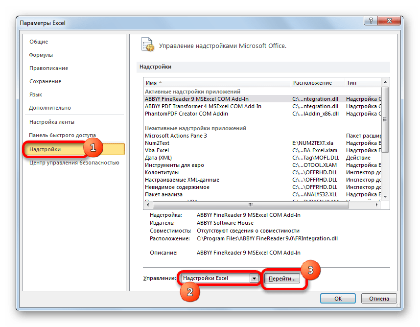
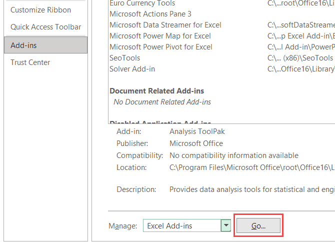
2. В активировавшемся окне параметров перемещаемся в подраздел «Надстройки». В самой нижней части окна находится поле «Управление». Нужно в нем переставить переключатель в позицию «Надстройки Excel», если он находится в другом положении. Вслед за этим жмем на кнопку «Перейти…».



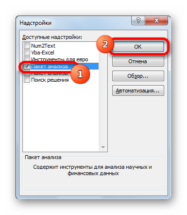
3. Запускается окно стандартных надстроек Excel. Около наименования «Пакет анализа» ставим флажок. Затем жмем на кнопку «OK».

После вышеуказанных действий надстройка Пакет анализа будет активирована и станет доступной во вкладке «Данные» Эксель. Теперь мы сможем использовать на практике инструменты описательной статистики.

Применение инструмента «Описательная статистика»

Теперь посмотрим, как инструмент описательная статистика можно применить на практике. Для этих целей используем готовую таблицу.

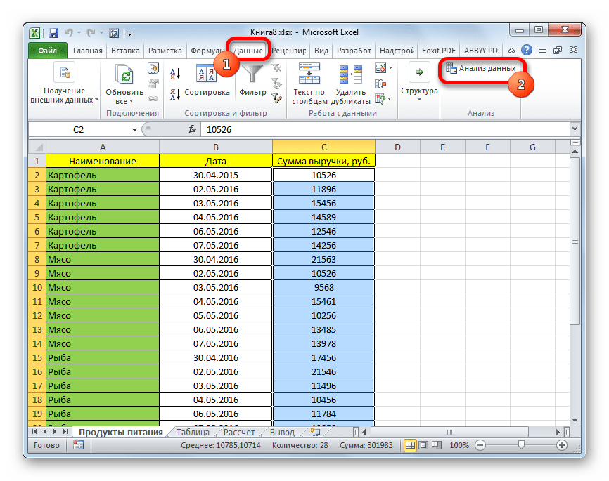
1. Переходим во вкладку «Данные» и выполняем щелчок по кнопке «Анализ данных», которая размещена на ленте в блоке инструментов «Анализ».



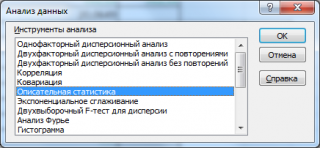
2. Открывается список инструментов, представленных в Пакете анализа. Ищем наименование «Описательная статистика», выделяем его и щелкаем по кнопке «OK».



3. После выполнения данных действий непосредственно запускается окно «Описательная статистика».

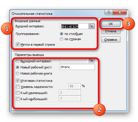
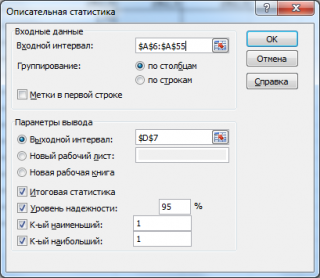
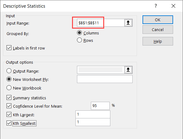
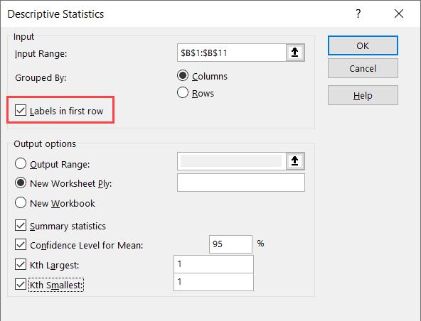
   В поле «Входной интервал» указываем адрес диапазона, который будет подвергаться обработке этим инструментом. Причем указываем его вместе с шапкой таблицы. Для того, чтобы внести нужные нам координаты, устанавливаем курсор в указанное поле. Затем, зажав левую кнопку мыши, выделяем на листе соответствующую табличную область. Как видим, её координаты тут же отобразятся в поле. Так как мы захватили данные вместе с шапкой, то около параметра «Метки в первой строке» следует установить флажок. Тут же выбираем тип группирования, переставив переключатель в позицию «По столбцам» или «По строкам». В нашем случае подходит вариант «По столбцам», но в других случаях, возможно, придется выставить переключатель иначе.

   

   Выше мы говорили исключительно о входных данных. Теперь переходим к разбору настроек параметров вывода, которые расположены в этом же окне формирования описательной статистики. Прежде всего, нам нужно определиться, куда именно будут выводиться обработанные данные:

   • Выходной интервал;
   • Новый рабочий лист;
   • Новая рабочая книга.

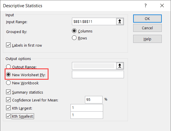
   В первом случае нужно указать конкретный диапазон на текущем листе или его верхнюю левую ячейку, куда будет выводиться обработанная информация. Во втором случае следует указать название конкретного листа данной книги, где будет отображаться результат обработки. Если листа с таким наименованием в данный момент нет, то он будет создан автоматически после того, как вы нажмете на кнопку «OK». В третьем случае никаких дополнительных параметров указывать не нужно, так как данные будут выводиться в отдельном файле Excel (книге). Мы выбираем вывод результатов на новом рабочем листе под названием «Итоги».

   Далее, если вы хотите чтобы выводилась также итоговая статистика, то нужно установить флажок около соответствующего пункта. Также можно установить уровень надежности, поставив галочку около соответствующего значения. По умолчанию он будет равен 95%, но его можно изменить, внеся другие числа в поле справа.

   Кроме этого, можно установить галочки в пунктах «K-ый наименьший» и «K-ый наибольший», установив значения в соответствующих полях. Но в нашем случае этот параметр так же, как и предыдущий, не является обязательным, поэтому флажки мы не ставим.

   После того, как все указанные данные внесены, жмем на кнопку «OK».



4. После выполнения этих действий таблица с описательной статистикой выводится на отдельном листе, который был нами назван «Итоги». Как видим, данные представлены сумбурно, поэтому их следует отредактировать, расширив соответствующие колонки для более удобного просмотра.



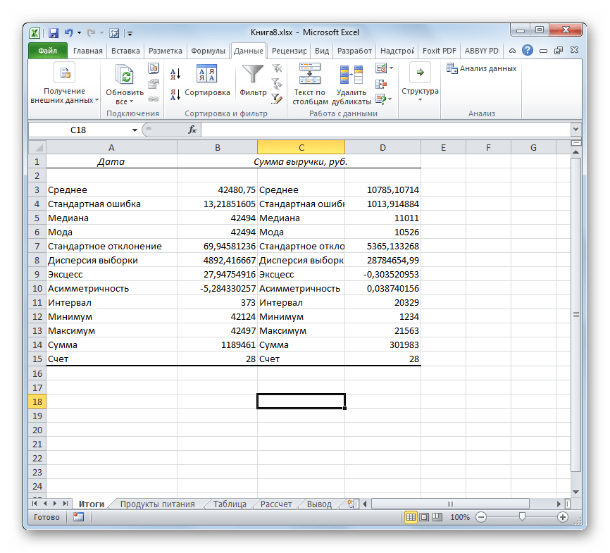
5. После того, как данные «причесаны» можно приступать к их непосредственному анализу. Как видим, при помощи инструмента описательной статистики были рассчитаны следующие показатели:
   • Асимметричность;
   • Интервал;
   • Минимум;
   • Стандартное отклонение;
   • Дисперсия выборки;
   • Максимум;
   • Сумма;
   • Эксцесс;
   • Среднее;
   • Стандартная ошибка;
   • Медиана;
   • Мода;
   • Счет.

Если какие-то из вышеуказанных данных для конкретного вида анализа не нужны, то их можно удалить, чтобы они не мешали. Далее производится анализ с учетом статистических закономерностей.

Урок: Статистические функции в Excel

Как видим, с помощью инструмента «Описательная статистика» можно сразу получить результат по целому ряду критериев, которые в ином случае рассчитывались с применением отдельно предназначенной для каждого расчета функцией, что заняло бы значительное время у пользователя. А так, все эти расчеты можно получить практически в один клик, использовав соответствующий инструмент — Пакета анализа.

Еще статьи по данной теме:

Помогла ли Вам статья?

Рассмотрим инструмент Описательная статистика, входящий в надстройку Пакет Анализа. Рассчитаем показатели выборки: среднее, медиана, мода, дисперсия, стандартное отклонение и др.

Задача

описательной статистики

(descriptive statistics) заключается в том, чтобы с использованием математических инструментов свести сотни значений

выборки

к нескольким итоговым показателям, которые дают представление о

выборке

.В качестве таких статистических показателей используются:

среднее

,

медиана

,

мода

,

дисперсия, стандартное отклонение

и др.

Опишем набор числовых данных с помощью определенных показателей. Для чего нужны эти показатели? Эти показатели позволят сделать определенные

статистические выводы о распределении

, из которого была взята

выборка

. Например, если у нас есть

выборка

значений толщины трубы, которая изготавливается на определенном оборудовании, то на основании анализа этой

выборки

мы сможем сделать, с некой определенной вероятностью, заключение о состоянии процесса изготовления.

Содержание статьи:

• Надстройка Пакет анализа;
• Среднее выборки

  ;

• Медиана выборки

  ;

• Мода выборки

  ;

• Мода и среднее значение

  ;

• Дисперсия выборки

  ;

• Стандартное отклонение выборки

  ;

• Стандартная ошибка

  ;

• Ассиметричность

  ;

• Эксцесс выборки

  ;

• Уровень надежности

  .

Надстройка Пакет анализа

Для вычисления статистических показателей одномерных

выборок

, используем

надстройку Пакет анализа

. Затем, все показатели рассчитанные надстройкой, вычислим с помощью встроенных функций MS EXCEL.

СОВЕТ

: Подробнее о других инструментах надстройки

Пакет анализа

и ее подключении – читайте в статье

Надстройка Пакет анализа MS EXCEL

.

Выборку

разместим на

листе

Пример

в файле примера

в диапазоне

А6:А55

(50 значений).

Примечание

: Для удобства написания формул для диапазона

А6:А55

создан

Именованный диапазон

Выборка.

В диалоговом окне

Анализ данных

выберите инструмент

Описательная статистика

.

После нажатия кнопки

ОК

будет выведено другое диалоговое окно,

в котором нужно указать:

• 
  входной интервал
  
  (Input Range) – это диапазон ячеек, в котором содержится массив данных. Если в указанный диапазон входит текстовый заголовок набора данных, то нужно поставить галочку в поле
  
  Метки в первой строке (
  
  Labels
  
  in
  
  first
  
  row
  
  ).
  
  В этом случае заголовок будет выведен в
  
  Выходном интервале.
  
  Пустые ячейки будут проигнорированы, поэтому нулевые значения необходимо обязательно указывать в ячейках, а не оставлять их пустыми;
• 
  выходной интервал
  
  (Output Range). Здесь укажите адрес верхней левой ячейки диапазона, в который будут выведены статистические показатели;
• 
  Итоговая статистика (
  
  Summary
  
  Statistics
  
  )
  
  . Поставьте галочку напротив этого поля – будут выведены основные показатели выборки:
  
  среднее, медиана, мода, стандартное отклонение
  
  и др.;
• Также можно поставить галочки напротив полей
  
  Уровень надежности (
  
  Confidence
  
  Level
  
  for
  
  Mean
  
  )
  
  ,
  
  К-й наименьший
  
  (Kth Largest) и
  
  К-й наибольший
  
  (Kth Smallest).

В результате будут выведены следующие статистические показатели:

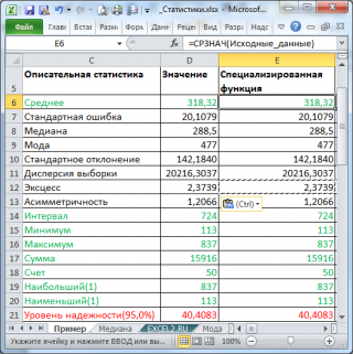
Все показатели выведены в виде значений, а не формул. Если массив данных изменился, то необходимо перезапустить расчет.

Если во

входном интервале

указать ссылку на несколько столбцов данных, то будет рассчитано соответствующее количество наборов показателей. Такой подход позволяет сравнить несколько наборов данных. При сравнении нескольких наборов данных используйте заголовки (включите их во

Входной интервал

и установите галочку в поле

Метки в первой строке

). Если наборы данных разной длины, то это не проблема — пустые ячейки будут проигнорированы.

Зеленым цветом на картинке выше и в

файле примера

выделены показатели, которые не требуют особого пояснения. Для большинства из них имеется специализированная функция:

• 
  Интервал
  
  (Range) — разница между максимальным и минимальным  значениями;
• 
  Минимум
  
  (Minimum) – минимальное значение в диапазоне ячеек, указанном во
  
  Входном интервале
  
  (см.

  статью про функцию
  
  МИН()
  
  );

• 
  Максимум
  
  (Maximum)– максимальное значение (см.

  статью про функцию
  
  МАКС()
  
  );

• 
  Сумма
  
  (Sum) – сумма всех значений (см.

  статью про функцию
  
  СУММ()
  
  );

• 
  Счет
  
  (Count) – количество значений во
  
  Входном интервале
  
  (пустые ячейки игнорируются, см.

  статью про функцию
  
  СЧЁТ()
  
  );

• 
  Наибольший
  
  (Kth Largest) – выводится К-й наибольший. Например, 1-й наибольший – это максимальное значение (см.

  статью про функцию
  
  НАИБОЛЬШИЙ()
  
  );

• 
  Наименьший
  
  (Kth Smallest) – выводится К-й наименьший. Например, 1-й наименьший – это минимальное значение (см.

  статью про функцию
  
  НАИМЕНЬШИЙ()
  
  ).

Ниже даны подробные описания остальных показателей.

Среднее выборки

Среднее

(mean, average) или

выборочное среднее

или

среднее выборки

(sample average) представляет собой

арифметическое среднее

всех значений массива. В MS EXCEL для вычисления среднего выборки используется функция

СРЗНАЧ()

.

Выборочное среднее

является «хорошей» (несмещенной и эффективной) оценкой

математического ожидания

случайной величины (подробнее см. статью

Среднее и Математическое ожидание в MS EXCEL

).

Медиана выборки

Медиана

(Median) – это число, которое является серединой множества чисел (в данном случае выборки): половина чисел множества больше, чем

медиана

, а половина чисел меньше, чем

медиана

. Для определения

медианы

необходимо сначала

отсортировать множество чисел

. Например,

медианой

для чисел 2, 3, 3,

4

, 5, 7, 10 будет 4.

Если множество содержит четное количество чисел, то вычисляется

среднее

для двух чисел, находящихся в середине множества. Например,

медианой

для чисел 2, 3,

3

,

5

, 7, 10 будет 4, т.к. (3+5)/2.

Если имеется длинный хвост распределения, то

Медиана

лучше, чем

среднее значение

, отражает «типичное» или «центральное» значение. Например, рассмотрим несправедливое распределение зарплат в компании, в которой руководство получает существенно больше, чем основная масса сотрудников.

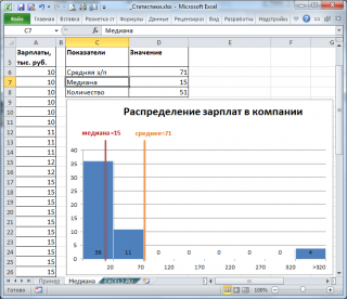
Очевидно, что средняя зарплата (71 тыс. руб.) не отражает тот факт, что 86% сотрудников получает не более 30 тыс. руб. (т.е. 86% сотрудников получает зарплату в более, чем в 2 раза меньше средней!). В то же время медиана (15 тыс. руб.) показывает, что

как минимум

у 50% сотрудников зарплата меньше или равна 15 тыс. руб.

Для определения

медианы

в MS EXCEL существует одноименная функция

МЕДИАНА()

, английский вариант — MEDIAN().

Медиану

также можно вычислить с помощью формул

=КВАРТИЛЬ.ВКЛ(Выборка;2) =ПРОЦЕНТИЛЬ.ВКЛ(Выборка;0,5).

Подробнее о

медиане

см. специальную статью

Медиана в MS EXCEL

.

СОВЕТ

: Подробнее про

квартили

см. статью, про

перцентили (процентили)

см. статью.

Мода выборки

Мода

(Mode) – это наиболее часто встречающееся (повторяющееся) значение в

выборке

. Например, в массиве (1; 1;

2

;

2

;

2

; 3; 4; 5) число 2 встречается чаще всего – 3 раза. Значит, число 2 – это

мода

. Для вычисления

моды

используется функция

МОДА()

, английский вариант MODE().

Примечание

: Если в массиве нет повторяющихся значений, то функция вернет значение ошибки #Н/Д. Это свойство использовано в статье

Есть ли повторы в списке?

Начиная с

MS EXCEL 2010

вместо функции

МОДА()

рекомендуется использовать функцию

МОДА.ОДН()

, которая является ее полным аналогом. Кроме того, в MS EXCEL 2010 появилась новая функция

МОДА.НСК()

, которая возвращает несколько наиболее часто повторяющихся значений (если количество их повторов совпадает). НСК – это сокращение от слова НеСКолько.

Например, в массиве (1; 1;

2

;

2

;

2

; 3;

4

;

4

;

4

; 5) числа 2 и 4 встречаются наиболее часто – по 3 раза. Значит, оба числа являются

модами

. Функции

МОДА.ОДН()

и

МОДА()

вернут значение 2, т.к. 2 встречается первым, среди наиболее повторяющихся значений (см.

файл примера

, лист

Мода

).

Чтобы исправить эту несправедливость и была введена функция

МОДА.НСК()

, которая выводит все

моды

. Для этого ее нужно ввести как

формулу массива

.

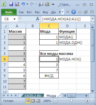
Как видно из картинки выше, функция

МОДА.НСК()

вернула все три

моды

из массива чисел в диапазоне

A2:A11

: 1; 3 и 7. Для этого, выделите диапазон

C6:C9

, в

Строку формул

введите формулу

=МОДА.НСК(A2:A11)

и нажмите

CTRL+SHIFT+ENTER

. Диапазон

C

6:

C

9

охватывает 4 ячейки, т.е. количество выделяемых ячеек должно быть больше или равно количеству

мод

. Если ячеек больше чем м

о

д, то избыточные ячейки будут заполнены значениями ошибки #Н/Д. Если

мода

только одна, то все выделенные ячейки будут заполнены значением этой

моды

.

Теперь вспомним, что мы определили

моду

для выборки, т.е. для конечного множества значений, взятых из

генеральной совокупности

. Для

непрерывных случайных величин

вполне может оказаться, что выборка состоит из массива на подобие этого (0,935; 1,211; 2,430; 3,668; 3,874; …), в котором может не оказаться повторов и функция

МОДА()

вернет ошибку.

Даже в нашем массиве с

модой

, которая была определена с помощью

надстройки Пакет анализа

, творится, что-то не то. Действительно,

модой

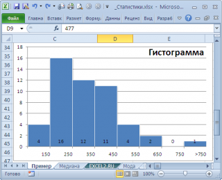
нашего массива значений является число 477, т.к. оно встречается 2 раза, остальные значения не повторяются. Но, если мы посмотрим на

гистограмму распределения

, построенную для нашего массива, то увидим, что 477 не принадлежит интервалу наиболее часто встречающихся значений (от 150 до 250).

Проблема в том, что мы определили

моду

как наиболее часто встречающееся значение, а не как наиболее вероятное. Поэтому,

моду

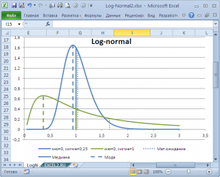
в учебниках статистики часто определяют не для выборки (массива), а для функции распределения. Например, для

логнормального распределения

мода

(наиболее вероятное значение непрерывной случайной величины х), вычисляется как

exp

(

m

—

s

²

)

, где m и s параметры этого распределения.

Понятно, что для нашего массива число 477, хотя и является наиболее часто повторяющимся значением, но все же является плохой оценкой для

моды

распределения, из которого взята

выборка

(наиболее вероятного значения или для которого плотность вероятности распределения максимальна).

Для того, чтобы получить оценку

моды

распределения, из

генеральной совокупности

которого взята

выборка

, можно, например, построить

гистограмму

. Оценкой для

моды

может служить интервал наиболее часто встречающихся значений (самого высокого столбца). Как было сказано выше, в нашем случае это интервал от 150 до 250.

Вывод

: Значение

моды

для

выборки

, рассчитанное с помощью функции

МОДА()

, может ввести в заблуждение, особенно для небольших выборок. Эта функция эффективна, когда случайная величина может принимать лишь несколько дискретных значений, а размер

выборки

существенно превышает количество этих значений.

Например, в рассмотренном примере о распределении заработных плат (см. раздел статьи выше, о Медиане),

модой

является число 15 (17 значений из 51, т.е. 33%). В этом случае функция

МОДА()

дает хорошую оценку «наиболее вероятного» значения зарплаты.

Примечание

: Строго говоря, в примере с зарплатой мы имеем дело скорее с

генеральной совокупностью

, чем с

выборкой

. Т.к. других зарплат в компании просто нет.

О вычислении

моды

для распределения

непрерывной случайной величины

читайте статью

Мода в MS EXCEL

.

Мода и среднее значение

Не смотря на то, что

мода

– это наиболее вероятное значение случайной величины (вероятность выбрать это значение из

Генеральной совокупности

максимальна), не следует ожидать, что

среднее значение

обязательно будет близко к

моде

.

Примечание

:

Мода

и

среднее

симметричных распределений совпадает (имеется ввиду симметричность

плотности распределения

).

Представим, что мы бросаем некий «неправильный» кубик, у которого на гранях имеются значения (1; 2; 3; 4; 6; 6), т.е. значения 5 нет, а есть вторая 6.

Модой

является 6, а среднее значение – 3,6666.

Другой пример. Для

Логнормального распределения

LnN(0;1)

мода

равна =EXP(m-s2)= EXP(0-1*1)=0,368, а

среднее значение

1,649.

Дисперсия выборки

Дисперсия выборки

или

выборочная дисперсия (

sample

variance

) характеризует разброс значений в массиве, отклонение от

среднего

.

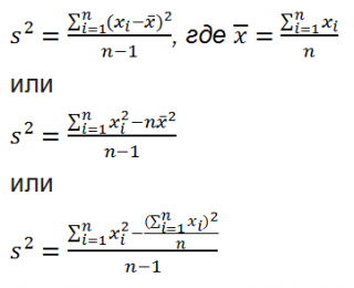
Из формулы №1 видно, что

дисперсия выборки

это сумма квадратов отклонений каждого значения в массиве

от среднего

, деленная на размер выборки минус 1.

В MS EXCEL 2007 и более ранних версиях для вычисления

дисперсии выборки

используется функция

ДИСП()

. С версии MS EXCEL 2010 рекомендуется использовать ее аналог — функцию

ДИСП.В()

.

Дисперсию

можно также вычислить непосредственно по нижеуказанным формулам (см.

файл примера

):

=КВАДРОТКЛ(Выборка)/(СЧЁТ(Выборка)-1) =(СУММКВ(Выборка)-СЧЁТ(Выборка)*СРЗНАЧ(Выборка)^2)/ (СЧЁТ(Выборка)-1)

– обычная формула

=СУММ((Выборка -СРЗНАЧ(Выборка))^2)/ (СЧЁТ(Выборка)-1)

–

формула массива

Дисперсия выборки

равна 0, только в том случае, если все значения равны между собой и, соответственно, равны

среднему значению

.

Чем больше величина

дисперсии

, тем больше разброс значений в массиве относительно

среднего

.

Размерность

дисперсии

соответствует квадрату единицы измерения исходных значений. Например, если значения в выборке представляют собой измерения веса детали (в кг), то размерность

дисперсии

будет кг

²

. Это бывает сложно интерпретировать, поэтому для характеристики разброса значений чаще используют величину равную квадратному корню из

дисперсии – стандартное отклонение

.

Подробнее о

дисперсии

см. статью

Дисперсия и стандартное отклонение в MS EXCEL

.

Стандартное отклонение выборки

Стандартное отклонение выборки

(Standard Deviation), как и

дисперсия

, — это мера того, насколько широко разбросаны значения в выборке

относительно их среднего

.

По определению,

стандартное отклонение

равно квадратному корню из

дисперсии

:

Стандартное отклонение

не учитывает величину значений в

выборке

, а только степень рассеивания значений вокруг их

среднего

. Чтобы проиллюстрировать это приведем пример.

Вычислим стандартное отклонение для 2-х

выборок

: (1; 5; 9) и (1001; 1005; 1009). В обоих случаях, s=4. Очевидно, что отношение величины стандартного отклонения к значениям массива у

выборок

существенно отличается.

В MS EXCEL 2007 и более ранних версиях для вычисления

Стандартного отклонения выборки

используется функция

СТАНДОТКЛОН()

. С версии MS EXCEL 2010 рекомендуется использовать ее аналог

СТАНДОТКЛОН.В()

.

Стандартное отклонение

можно также вычислить непосредственно по нижеуказанным формулам (см.

файл примера

):

=КОРЕНЬ(КВАДРОТКЛ(Выборка)/(СЧЁТ(Выборка)-1)) =КОРЕНЬ((СУММКВ(Выборка)-СЧЁТ(Выборка)*СРЗНАЧ(Выборка)^2)/(СЧЁТ(Выборка)-1))

Подробнее о

стандартном отклонении

см. статью

Дисперсия и стандартное отклонение в MS EXCEL

.

Стандартная ошибка

В

Пакете анализа

под термином

стандартная ошибка

имеется ввиду

Стандартная ошибка среднего

(Standard Error of the Mean, SEM).

Стандартная ошибка среднего

— это оценка

стандартного отклонения

распределения

выборочного среднего

.

Примечание

: Чтобы разобраться с понятием

Стандартная ошибка среднего

необходимо прочитать о

выборочном распределении

(см. статью

Статистики, их выборочные распределения и точечные оценки параметров распределений в MS EXCEL

) и статью про

Центральную предельную теорему

.

Стандартное отклонение распределения выборочного среднего

вычисляется по формуле σ/√n, где n — объём

выборки, σ — стандартное отклонение исходного

распределения, из которого взята

выборка

. Т.к. обычно

стандартное отклонение

исходного распределения неизвестно, то в расчетах вместо

σ

используют ее оценку

s

—

стандартное отклонение выборки

. А соответствующая величина s/√n имеет специальное название —

Стандартная ошибка среднего.

Именно эта величина вычисляется в

Пакете анализа.

В MS EXCEL

стандартную ошибку среднего

можно также вычислить по формуле

=СТАНДОТКЛОН.В(Выборка)/ КОРЕНЬ(СЧЁТ(Выборка))

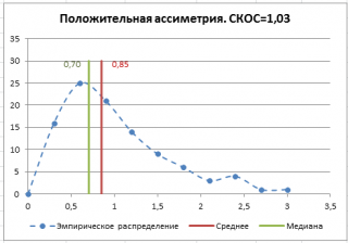
Асимметричность

Асимметричность

или

коэффициент асимметрии

(skewness) характеризует степень несимметричности распределения (

плотности распределения

) относительно его

среднего

.

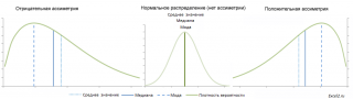
Положительное значение

коэффициента асимметрии

указывает, что размер правого «хвоста» распределения больше, чем левого (относительно среднего). Отрицательная асимметрия, наоборот, указывает на то, что левый хвост распределения больше правого.

Коэффициент асимметрии

идеально симметричного распределения или выборки равно 0.

Примечание

:

Асимметрия выборки

может отличаться расчетного значения асимметрии теоретического распределения. Например,

Нормальное распределение

является симметричным распределением (

плотность его распределения

симметрична относительно

среднего

) и, поэтому имеет асимметрию равную 0. Понятно, что при этом значения в

выборке

из соответствующей

генеральной совокупности

не обязательно должны располагаться совершенно симметрично относительно

среднего

. Поэтому,

асимметрия выборки

, являющейся оценкой

асимметрии распределения

, может отличаться от 0.

Функция

СКОС()

, английский вариант SKEW(), возвращает коэффициент

асимметрии выборки

, являющейся оценкой

асимметрии

соответствующего распределения, и определяется следующим образом:

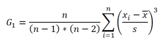
где n – размер

выборки

, s –

стандартное отклонение выборки

.

В

файле примера на листе СКОС

приведен расчет коэффициента

асимметрии

на примере случайной выборки из

распределения Вейбулла

, которое имеет значительную положительную

асимметрию

при параметрах распределения W(1,5; 1).

Эксцесс выборки

Эксцесс

показывает относительный вес «хвостов» распределения относительно его центральной части.

Для того чтобы определить, что относится к хвостам распределения, а что к его центральной части, можно использовать границы μ +/-

σ

.

Примечание

: Не смотря на старания профессиональных статистиков, в литературе еще попадается определение

Эксцесса

как меры «остроконечности» (peakedness) или сглаженности распределения. Но, на самом деле, значение

Эксцесса

ничего не говорит о форме пика распределения.

Согласно определения,

Эксцесс

равен четвертому

стандартизированному моменту:

Для

нормального распределения

четвертый момент равен 3*σ

⁴

, следовательно,

Эксцесс

равен 3. Многие компьютерные программы используют для расчетов не сам

Эксцесс

, а так называемый Kurtosis excess, который меньше на 3. Т.е. для

нормального распределения

Kurtosis excess равен 0. Необходимо быть внимательным, т.к. часто не очевидно, какая формула лежит в основе расчетов.

Примечание

: Еще большую путаницу вносит перевод этих терминов на русский язык. Термин Kurtosis происходит от греческого слова «изогнутый», «имеющий арку». Так сложилось, что на русский язык оба термина Kurtosis и Kurtosis excess переводятся как

Эксцесс

(от англ. excess — «излишек»). Например, функция MS EXCEL

ЭКСЦЕСС()

на самом деле вычисляет Kurtosis excess.

Функция

ЭКСЦЕСС()

, английский вариант KURT(), вычисляет на основе значений выборки несмещенную оценку

эксцесса распределения

случайной величины и определяется следующим образом:

Как видно из формулы MS EXCEL использует именно Kurtosis excess, т.е. для выборки из

нормального распределения

формула вернет близкое к 0 значение.

Если задано менее четырех точек данных, то функция

ЭКСЦЕСС()

возвращает значение ошибки #ДЕЛ/0!

Вернемся к

распределениям случайной величины

.

Эксцесс

(Kurtosis excess) для

нормального распределения

всегда равен 0, т.е. не зависит от параметров распределения μ и σ. Для большинства других распределений

Эксцесс

зависит от параметров распределения: см., например,

распределение Вейбулла

или

распределение Пуассона

, для котрого

Эксцесс

= 1/λ.

Уровень надежности

Уровень

надежности

— означает вероятность того, что

доверительный интервал

содержит истинное значение оцениваемого параметра распределения.

Вместо термина

Уровень

надежности

часто используется термин

Уровень доверия

. Про

Уровень надежности

(Confidence Level for Mean) читайте статью

Уровень значимости и уровень надежности в MS EXCEL

.

Задав значение

Уровня

надежности

в окне

надстройки Пакет анализа

, MS EXCEL вычислит половину ширины

доверительного интервала для оценки среднего (дисперсия неизвестна)

.

Тот же результат можно получить по формуле (см.

файл примера

):

=ДОВЕРИТ.СТЬЮДЕНТ(1-0,95;s;n)

s —

стандартное отклонение выборки

, n – объем

выборки

.

Подробнее см. статью про

построение доверительного интервала для оценки среднего (дисперсия неизвестна)

.

Descriptive statistics with excel is a popular way to describe your data. It makes the tons of formula became easier just by simple click and drop.

Years ago, I do the formula one by one and find the statistic value that I need. It is really uncomfortable, is not it?

You have to remember the correct formula of your data and choose the right formula because perhaps there is more than one similar formula for one statistic value.

Look at he picture I present below. This is what you will using descriptive statistics with excel by typing the formula one by one

There are 7 formulas that excel provide to you to generate the variance of your data. My question is, which one will you use?

Still, writing one by one formula to summarize the statistic value that you need? Well, keep reading!

Microsoft Excel is a phenomenal software developed by Microsoft helping Billions of human to solve their problems. Excel helps us to makes almost our calculation problem easier included statistics.

Why using descriptive statistics in excel?

If you are wondering why you should Microsoft Excel to process your statistical data, let me tell you these interesting facts!

1. The user interface is so friendly

Yes, Microsoft Excel interface is so friendly so almost every user could use it without any meaningful problem. You may use it through simple steps and clicks to produce the output that you want.

2. No coding needed

Usually, almost all statistical software needs to code the form. But, Excel does not require you to code anything. You just need to know the simple formula or use the toolbar that will help you to finish the job.

3. Easy to interpret

The output is served simply so we may see it and understand what the output is. If you did not strong statistical basics, do not worry. It’s just basic formula which you may learn in your study.

Before using Microsoft Excel to process your data, you must activate the data analysis toolpak to makes your job easier.

Follow these simple steps!

1. Activate the data analysis toolpak, go to file >> options

2. Choose add ins >> analysis toolpak

3. Ok

Now, you will have the tools that you need to make your works easier and faster. By using this toolpak, you do not have to input every single formula that you need. Now, let’s calculate the descriptive statistics in excel

Already have your data set? Let’s do the analysis. Here is the steps!

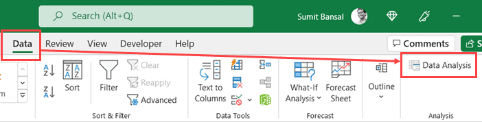
1. Go to Data >> data analysis

2. You’ll see many statistical options there, choose descriptive statistics >> ok

3. In the popup window, you have several fields that you have to fill

• Input range: block the data you want to analyze
• Grouped by: whether the data is grouped in columns or rows
• Labels in the first row: if the blocked data has labels in the first row, check this
• Output options: where the output will be displayed
• Summary statistics: if you want to do descriptive statistics analysis
• The confidence level for mean: if you want to show confidence level for mean
• Kth largest: if you want to show the data in “k”th largest
• Kth smallest: if you want to show the data in “k”th smallest

4. Click Ok

5. See the magic happens!

Interpretation of Descriptive Statistics Output in Excel

1. Mean = 7,434. In average, there are 7,434 poor people in these 12 areas

2. Standard error = 468.412. This value indicates that the sample we chose has a fairly high distribution of the population mean.

3. Median = 7,575. This value indicates that the middle numbers of poor people based on the sample we use are 7,575 people.

4. Mode = 8000. This value shows that the most number of poor people based on the sample we have is 8000 people.

5. Standard deviation = 1622. This value indicates that the sample values ​​that we use are spread far enough from the mean value.

6. Kurtosis = -0.68485. Because the value of kurtosis is smaller than 3, we can conclude that the sample used is platicurtic distribution (tends to be flat).

7. Skewness = -0.12018. Because the skewness value is smaller than zero, we can conclude that the data tends to be left inclined or left skewed.

8. Range = 5100. This value indicates that the difference between the regions with the highest number of poor people and the lowest number of poor people is 5100 people.

9. Minimum = 4900. This value shows the lowest number of poor people is 4900 people in the L area.

10. Maximum = 10,000. This value shows that the highest number of poor people is 10,000 people in J area.

11. Sum = 89,210. This value indicates that the total number of poor people based on the data used was 89,210 people.

12. Count = 12. This value indicates the amount of data used is 12.

13. Confidence level = 1030,968. It’s quite difficult to understand, right? Okay, keep reading.

Confidence interval means we will predict a value in the form of a range. In this case, we need upper values ​​and lower values.

In the descriptive statistics feature in Microsoft Excel, they only provide one value, and this figure is very far from the mean.

The confidence level value that appears is a value that can be used to get the upper and lower limits of the confidence interval you are using.

If you want to get the upper limit, you simply add an average to the value of the confidence level. The following calculations. Check the picture below!

If you want to get a lower bound value, you can simply reduce the average value with that confidence level. Consider the following picture.

Now, let’s make the interpretation of this value!

With a confidence level of 95 percent, the average number of poor people in the 12 regions is 6,403 to 8,465 people.

The Disadvantage of Using Excel For Descriptive Statistics

1. The formula is limited

Although the formula is super easy just by drag and click, the numbers of excel formula in the statistical process are limited.

Excel provided not much formula so the user can use to do data processing. But, Excel is the best tool to study statistical computing if you want to be advanced in the future.

2. It is only for numerical data

It’s sad but if you are using categorical or non-numeric data, probably excel is not for your research. Excel only read the data in numeric format. Even you transform it into numerical form, it’s quite difficult to read the output.

3. It is only for single variable analysis

Conclusion

Overall, the steps of using descriptive statistics in excel are:

1. Prepare the data set.

2. Activate analysis toolpak add-ins add options menu.

3. Choose the descriptive statistics at the data analysis menu.

4. Check the statistic value that you want to generate.

5. Click Ok.

6. Do not forget to make the output interpretation.

If you want to do more advanced analysis by software, I recommend you to check the descriptive statistics on spss article. You will find an easier way to produce the descriptive statistics even for the numerical or categorical data set.

If you’re working with large datasets in excel, getting Descriptive Statistics for this data set could be useful.

Descriptive Statistic quickly summarizes your data and gives you a few data points that you can use to quickly understand the entire data set.

While you can also calculate each of these statistical values individually, using the descriptive statistics option in Excel quickly gives you all this data in one single place (and it’s a lot faster than using different formulas to calculate different values).

In this short tutorial, I will show you how to get Descriptive Statistics in Excel.

Descriptive Statistics in Excel

To get the Descriptive Statistics in Excel, you need to have the Data Analysis Toolpak enabled.

You can check whether you already have it enabled by going to the Data tab.

If you see the Data Analysis option in the Analysis group, you already have it enabled (and you can skip the next section and go directly to the ‘Getting Descriptive Analysis’ section).

In case you do not see the data analysis option in the data tab, follow the steps in the next section to enable it.

Enabling Data Analysis Toolpak

Below are the steps to enable the Data Analysis Toolpak in Excel:

1. Open any Excel document
2. Click the File tab

1. Click on Options. This will open the Excel Options dialog box

1. In the Excel Options dialog box, click on Add-ins in the left pane

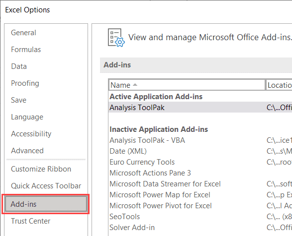
1. From the Manage drop-down (which is at the bottom of the dialog box), select ‘Excel Add-ins’

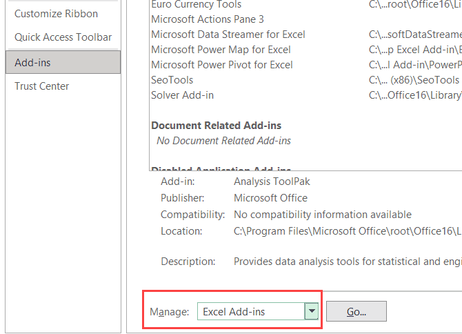
1. Click on the Go button

1. In the Add-ins dialog box that shows up, check the Analysis Toolpak option

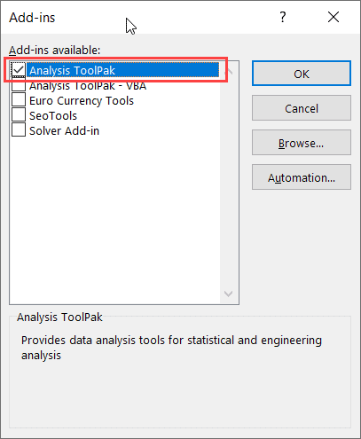
1. Click OK

The other steps would enable the Data Analysis toolpak and you will be able to use it on all your Excel Workbooks.

Getting the Descriptive Analysis

Now that the Data Analysis Toolpak is enabled, let’s see how to get the descriptive statistics using it.

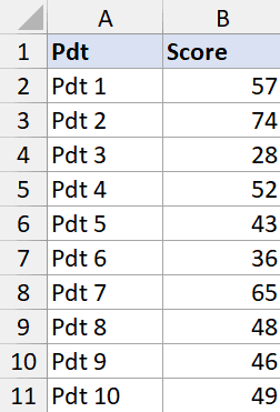
Suppose you have a data set as shown below where I have the sales data of different products of a company. For this data, I want to get descriptive statistics.

Below are the steps to do this:

1. Click the Data tab
2. In the Analysis group, click on Data Analysis

1. In the Data Analysis dialog box that opens, click on Descriptive Statistics

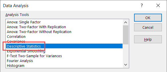
1. Click OK
2. In the Descriptive Statistics dialog box, specify the input range that has the data. Note that I have only used Column B as the data source (as you can only use numeric data as the input here)

1. If your data has headers, check the ‘Labels in first row’ option

1. Select the New Worksheet Ply option (this will give the result in a new sheet)

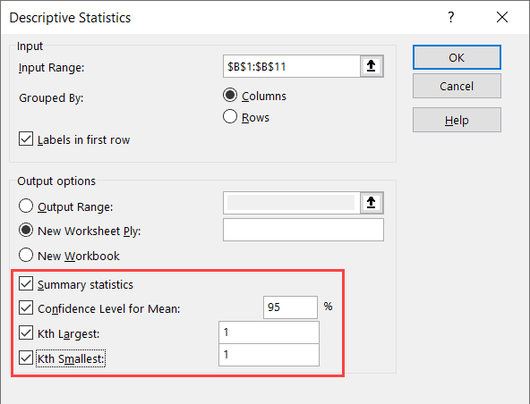
1. Select the statistics options you want (you need to select atleast one, and can select all four)

1. Click OK

The above steps would insert a new sheet and you will get the statistics as shown below:

Note that you can specify the following in step 8:

1. Confidence Level for mean – the default is 95%, but you can change the value
2. Kth Largest – the default is 1, but you can change it. If you enter 3 here, it will give you the third largest value from the dataset
3. Kth Smallest – the default is 1, but you can change it. If you enter 3 here, it will give you the third smallest value from the dataset

Note that the resulting values you get are static values.

In case your original data changes and you again want to get the Descriptive Statistics, you will have to repeat the above steps again.

So this is how you can quickly get Descriptive Statistics in Microsoft Excel.

I hope you found this tutorial useful.

Other Excel Tutorials you may also like:

• How to Calculate Standard Deviation in Excel
• How to Calculate PERCENTILE in Excel
• Calculating Weighted Average in Excel.
• Calculating CAGR in Excel
• How to Calculate Correlation Coefficient in Excel
• Calculate the Coefficient of Variation (CV) in Excel

DESCRIPTIVE STATISTICS
USING EXCEL AND STATA

(Excel
2003 and Stata 10.0+)

If you
do not see the menu on the left click here to see it

These
notes are meant to
provide a general overview on how to input data in Excel and Stata and how to
perform basic data analysis by looking at some descriptive statistics using
both programs.

Excel

To open Excel
in windows go Start — Programs — Microsoft Office — Excel

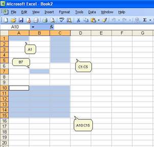
When it opens
you will see a blank worksheet, which consists of alphabetically titled columns
and numbered rows. Each cell is referenced by its coordinates of columns and
rows, for example A1 is the cell located in column A and row 1; B7 is the cell
in column B and row 7. You can reference a range of cells, for example C1:C5
are cells in columns C and rows 1 to 5. You can also reference a matrix,
A10:C15, are cells in columns A, B and C and rows 10 to 15.

Excel has 256
columns and 65,536 rows.

There are
some shortcuts to move within the current sheet:

·        
«Home»
moves to the first column in the current row

·        
«End
— Right Arrow» moves to the last filled cell in the current row

·        
«End
— Down Arrow» moves to the last filled cell in the current column

·        
«Ctrl-Home»
moves to cell A1

·        
«Ctrl-End»
moves to the last cell in your document (not the last cell of the current
sheet)

·        
«Ctrl-Shift-End»
selects everything between the active cell to the last cell in the document

To
select a cell :

·        
Click
on a cell (i.e. A10), hold the shift key, click on
another cell (C15) to select the cells between A10 and C15.

·        
You
can also click on a cell and drag the mouse to the desire range

·        
To
select not-adjacent cells, click on a cell, press ctrl and select another cell
or range of cells.

Excel
stores your work in a workbook, each workbook has one or more worksheets
(and/or charts) which you can view by clicking on the sheet tab (lower left corner
of the active (current) sheet).

Entering
data

You
can type anything on a cell, in general you can enter text (or labels),
numbers, formulas (starting with the «=» sign), and logical values (as in
«true» or «false»).

Click
on a cell and start typing, once you finish typing press «enter» (to move to
the next cell below) or «tab» (to move to the next cell to the right)

You
can write long sentences in one single cell but you may see it partially
depending on the column width of the cell (and whether the adjacent column is
full). To adjust the width of a column go to Format — Column — Width or select
«AutoFit Selection».

Numbers
are assumed to be positive, if you need to enter a negative value use the minus
sign («-«) or enclose the number in parentheses («(number)»).

If
you need to enter percentages, dollar sign, or any other symbol to identify the
number just add the «%» or «$». You can also enter the number and change its
format using the menu: Format — Cell and select the «number» tab which has all
the different formats.

Dates
are automatically stored as mm/dd/yyyy
(or the default format if changed) but there is some flexibility here. Enter
month and number and excel will enter the date in the default format. If you
press «ctrl» and «;» (Crtl-;) excel will enter the
current date.

Time
is also entered in a default format. Enter «5 pm», excel will write «5:00 PM».
To enter the current time press «ctrl» and «:» (Ctrl-:)

To
practice enter the following table (these data are made-up, not real)

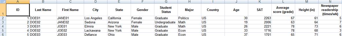
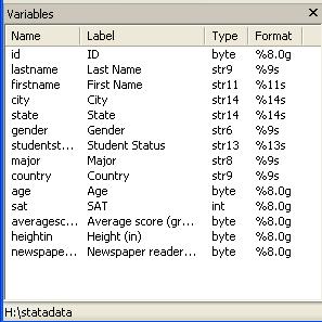
Each
column has a list of items. Column A has IDs, column B
has last names of students and so on.

Let»s say for example you do not want
capital letters for the columns «Last Name» and «First Name». You do not want
«SMITH» you want «Smith». Two options, you can re-type all the names or you can
use the following formula (IMPORTANT: All formulas start
with the equal «=» sign):

=PROPER(cell with the text you want to change)

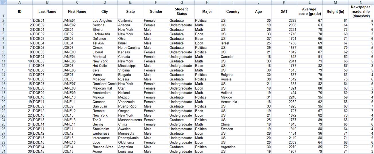
To
get the full table:Click here to get it.

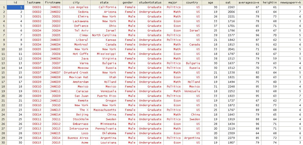
The
full table should look like this. This is a made up table, it is just a
collection of random info and data.

Exploring data in excel

Descriptive
statistics (using excel»s data analysis tool)

Generally
one of the first things to do with new data is to get to know it by asking some
general questions like but not limited to the following:

·        
What
variables are included? What information are we getting?

·        
What
is the format of the variables: string, numeric, etc.?

·        
What
type of variables: categorical, continuous, and discrete?

·        
Is
this sample or population data?

After looking
at the data you may want to know

·        
How
many males/females?

·        
What
is the average age?

·        
How
many undergraduate/graduates students?

·        
What
is the average SAT score? It is the same for graduates and undergraduates?

·        
Who
reads the newspaper more frequently: men or women?

You
can start answering some of these questions by looking directly at the table,
for some other questions you may have to do some calculations by obtaining a
set of descriptive statistics. These statistics are a collection of
measurements of two things: location and variability. Location
tells you the central value (the mean is the most common measure of this) of
your variables. Variability refers to the spread of the data from the center
value (i.e. variance, standard deviation). Statistics is basically the study of
what causes such variability.

Let»s
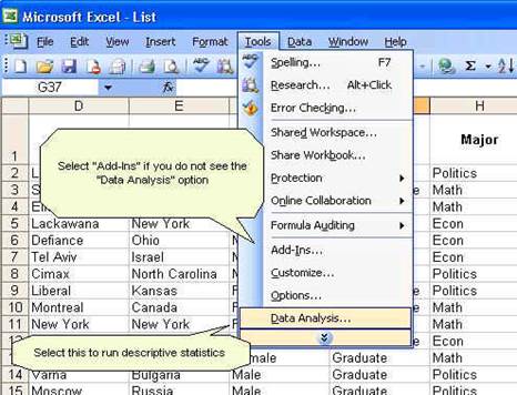
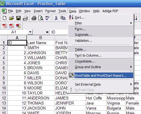
get some descriptive statistics for this data. In excel go to Tools — Data
Analysis. If you do not see «data analysis» option you need to install it, go
to Tools — Add-Ins, a window will pop-up and check the «Analysis ToolPack» option, then press OK. Try running data analysis
again.

For Excel 2007 see http://office.microsoft.com/en-us/excel/HP100215691033.aspx

For Excel 2003 see http://office.microsoft.com/en-us/excel/HP011277241033.aspx 

In
the pop-up window select «Descriptive Statistics» click OK.

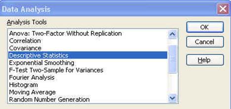
Another
window will pop-up

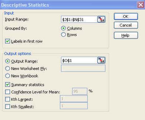
Let»s
check this window:

Input Range: This is to select the data you want
to analyze.

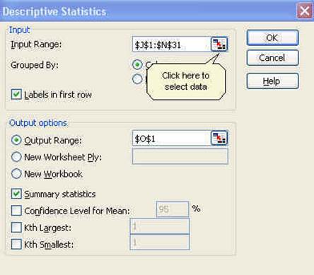
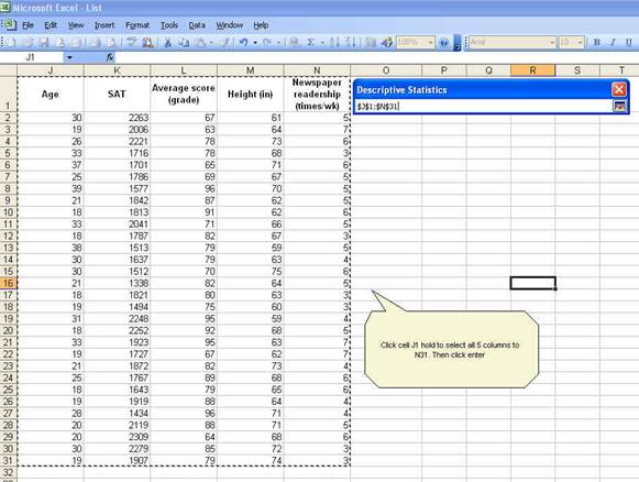
Once
you click in the input range you need to select the cells you want to analyze.

Back
to the window

Since
we include the labels in first row make sure to check that option. For
the output option which is the place where excel will enter the results
select O1 or you can select a new worksheet or even new workbook.

Check
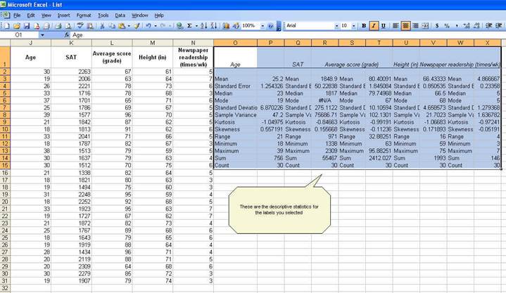
«Summary statistics» and the press OK. You will get the following:

While
the whole descriptive statistics cells are selected go to Format—Cells to
change all numbers to have one decimal point. When you get the «format cells»
window, select the following:

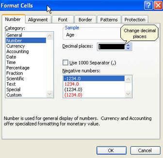
Click OK. All numbers should now have one
decimal as follows:

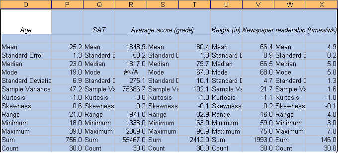
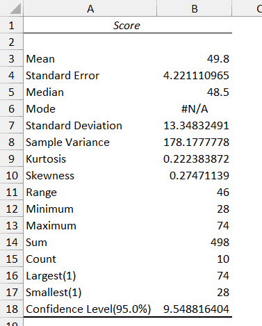
Now we know something about our data.

The
average student in this sample is 25.2 years, has a SAT score of 1848.9, got a
grade of 80.4, is 66.4 inches tall and reads the newspaper 4.9 times a week. We
know this by looking at the «mean» value on each variable.

The
mean is the sum of the observations divided by the total number of
observations. It is the most common indicator of central tendency of a
variable. If you look at the last two rows: «Sum» and «Count» you can estimate
the mean dividing «Sum» by «Count» (sum/count). You can also calculate the mean
using the function below (IMPORTANT: All functions start
with the equal «=» sign):

«Sum» refers to the sum of all the values in a range of
values. For age means the sum of the ages of all students. The excel function
for sum is:

=SUM(range of cells with the values of interest)

«Count» refers to the count of cell that contain values
(numbers). The function is:

=COUNT(range of cells with the values of interest)

«Min» is the lowest value in an array of values. The
function is:

=MIN(range of cells with the values of interest)

«Max»
is the largest value in an array of values. The function is:

=MAX(range of cells with the values of interest)

The «Standard
Error» (SE) indicates how close the sample mean is from the «true»
population mean. The average age of 25.2 years is just an estimate of this
sample of students but it can vary had you used a different set of students.
The standard error is calculated by dividing the standard deviation of the
population (or the sample) by the square root of the total number of
observations. The SE can be used to roughly define a range of certainty for the
mean. Using «age»:

Z	% Certainty	Lower bound	Upper bound
1 (0.99)	68%	23.9	26.5
2 (1.96)	95%	22.7	27.7
3 (2.58)	99%	21.4	29.0

Lower:  Mean—(SE*Z) for example 25.2—(1.3 * 2) =
22.7

Upper:  Mean + (SE*Z) for example 25.2 + (1.3 * 2) =
27.7

·        
You are 68% certain that the average age is
between 23.9 and 26.5 years old

·        
You are 95% certain that the average age is between
22.7 and 27.7 years old

·        
You are 99% certain that the average age is
between 21.4 and 29.0 years old

Note
that the more certainty wider the gap.

The
median is another measure of central tendency. To get
the median you have to order the data from lowest to highest. The median is the
number in the middle.  If the number of
cases is odd the median is the single value, for an even number of cases the
median is the average of the two numbers in the middle. The excel function is:

=MEDIAN(range of cells with the values of interest)

The
mode refers to the most frequent, repeated or common
number in the data. By age there are more students 19 years old in the sample
than any other group. In the SAT scores the mode is «#N/A» which means that all
values are unique. The excel function is:

=MODE(range of cells with the values of interest)

Range is a measure of dispersion. It is
simple the difference between the largest and smallest value, «max»—«min».

The
sample variance measures the dispersion of
the data from the mean. It is the simple mean of the squared distance from the
mean. It is calculated by:

SV
= sum of (X-mean of X)² / Number of observation minus 1

Higher
variance means more dispersion from the mean. 
The excel function is:

=VAR(range of cells with the values of interest)

The
standard deviation is the squared root of the
variance. Indicates how close the data is to the mean. Assuming a normal
distribution, 68% of the values are within 1 sd from
the mean, 95% within 2 sd and 99% within 3 sd. The
excel formula is:

=STDEV(range of cells with the values of interest)

Skewness measures the asymmetry of the data,
when in an otherwise normal curve one of the tails is longer than the other. It
is a roughly test for normality in the data (by dividing it by the SE). If it
is positive there is more data on the left side of the curve (right skewed, the
median and the mode are lower than the mean). A negative value indicates that
the mass of the data is concentrated on the right of the curve (left tail is
longer, left skewed, the median and the mode are higher than the mean). A
normal distribution has a skew of 0. Skewness can
also be estimated with the following function:

=SKEW(range of cells with the values of interest)

Kurtosis. The current view of kurtosis argues
that it measures the peak of a distribution. According to
Peter Westfall, that view is not quite correct. His article «Kurtosis as
Peakedness, 1905—2014. R.I.P.» (http://www.ncbi.nlm.nih.gov/pmc/articles/PMC4321753/)
makes a compelling case against the current perception. In Westfall»s view, the
peak, or lack-thereof, is a symptom rather than a characteristic that shows the
presence of outliers. High kurtosis may suggest the presence of outliers.
Technically speaking, kurtosis focuses more on the tails for the distribution
than the peak, so positive kurtosis indicates too few cases in the tails or a
tall distribution (leptokurtic), negative kurtosis too many cases in the tails
or a flat distribution (platykurtic). A normal
distribution has a kurtosis of 0 (given a correction of -3, otherwise it will
have a kurtosis of 3). The excel function for kurtosis is:

=KURT(range of cells with the values of interest)

—Thank
you to Peter Westfall for useful feedback.

Exploring data using pivot tables

To
explore the data by groups you can sort the columns for the variables you want
(for example gender, or major or country, etc.) and obtain descriptive statistics
by selecting only the range of values that cover particular group. You can also
use pivot tables.

Let»s
say you are interested on looking at the average SAT score by gender and
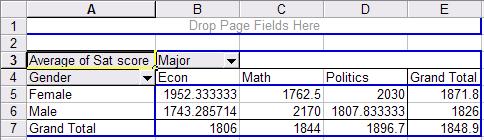
student»s major. Let»s make the following crosstabulation

In
the excel menu go to Menu—PivtoTable and PivotChart
Report:

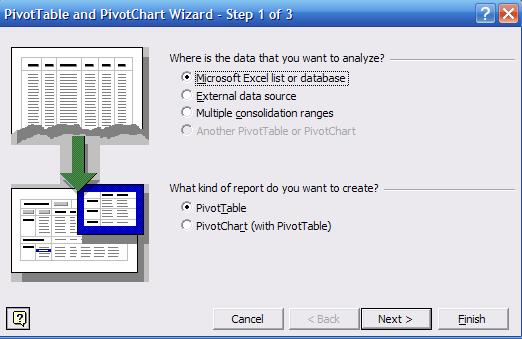
The
pivot wizard will walk you through the process, this is the first window

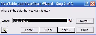
Press
«Next». In step 2 select the range for the range of all values as in the
following picture:

In
step 3 select «New worksheet» and press «Layout»

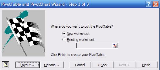
This
is where you make the pivot table:

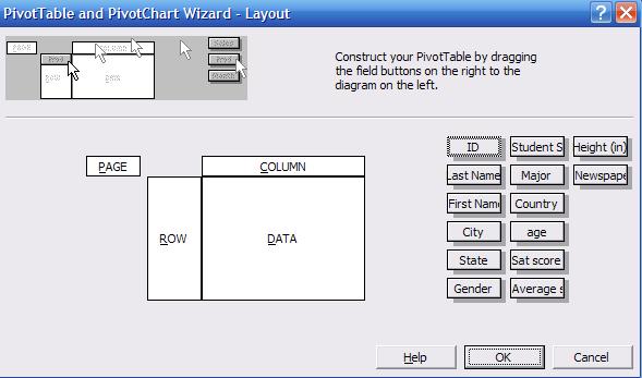
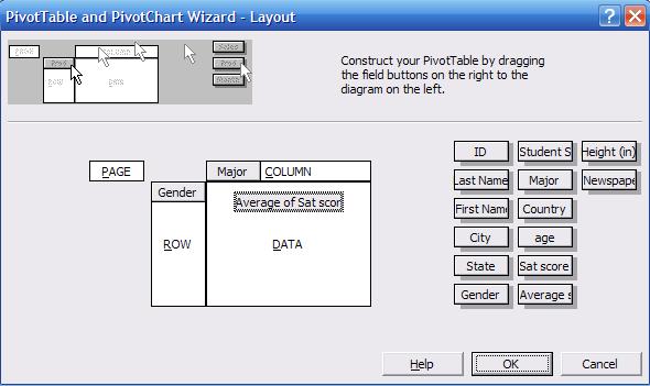
On
the right side of the wizard layout you can see the list of all variables in
the data. Click and drag «Gender» into the «ROW» area. Click and drag «Major»
into the «COLUMN» area, and click and drag «Sat score» into the «DATA» area.
The wizard layout should look like this:

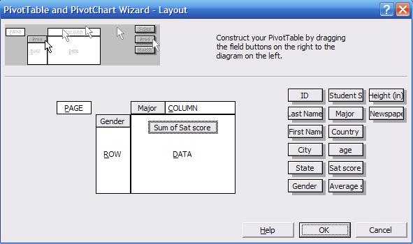
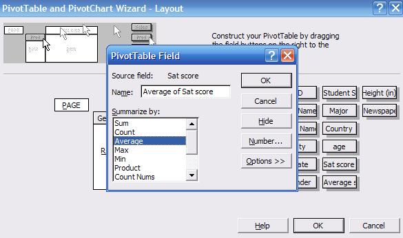
In
the «DATA» area double-click on «Sum of Sat score», a new window will pop-up
select «Average» and click OK.

The
wizard layout should look like this. Click OK, in the wizard window step 3
click «Finish»

In
a new worksheet you will see the following (the pivot table window was moved to
save some space).

This
is a crosstabulation between gender and major. Each cell
represents the average SAT score for a student according to gender and major.
For example a female student with an econ major has an average SAT score of
1952 (cell B5 in the picture) while a male student also with an econ major has
1743 (B6). Overall econ major students have an average SAT score of 1806 (B7) .
In general, female students have an average SAT score in this sample of 1871.8
(E5) while male students 1826 (E6).

For
more information on pivot tables go to the following site.

http://www.microsoft.com/dynamics/using/excel_pivot_tables_collins.mspx

For
graphing in excel we recommend the following links.

(Histograms)

http://office.microsoft.com/en-us/excel/HA011109481033.aspx

(Histograms)

http://www.physics.upenn.edu/~uglabs/Histograms-with-Excel.pdf

http://www.fgcu.edu/support/office2000/excel/charts.html

http://www.csubak.edu/~jross/classes/GS390/Spreadsheets/ExcelCharts/CreateChart.htm

http://www.ncsu.edu/labwrite/res/gt/gt-bar-home.html

(Error bars)

http://peltiertech.com/Excel/ChartsHowTo/ErrorBars.html

(Error bars)

http://mtsu32.mtsu.edu:11009/Graphing_Guides/Excel_Guide_Line_Means.htm

One-way ANOVA using excel

Let»s
say you want to explore whether there is a relationship between the average
score (grade) of each student and his/her major. In the sample we have three
majors: Econ, Math and Politics. The grades are the final grades for the entire
academic year.

To
do this we use one-way ANOVA, which stands for «analysis of variance». ANOVA
«is a broad class of techniques for identifying and measuring the various
sources of variation within a collection of data» (Kachigan,
p. 273, 1986). It is closely related to regression analysis but with the
following difference: «[w]e can think of the analysis of variance technique as
testing hypotheses about the presence of relationships between predictor
and criterion variables, regression analysis as describing the nature of
those relationships, and r² as measuring the strength of the
relationships» (ibidem.) In other words, ANOVA
«tests whether the means of y [grades
in this example] differ across categories of x [majors]» (Hamilton, p. 149)

With
the above in mind, let»s see if there is a relationship between student»s
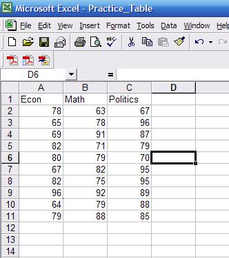
majors and student»s final grades. First we need to rearrange the data so excel
can run the ANOVA. Using only the columns «major» and «average score (grade)».
Copy and paste both columns into a new sheet, sort by major (Data—Sort,
select the column for major and sort ascending) separate by group. Final table
should look like this..

Go
to Tools — Data Analysis, in the pop-up window select «Anova:
Single Factor», the following screen will pop-up

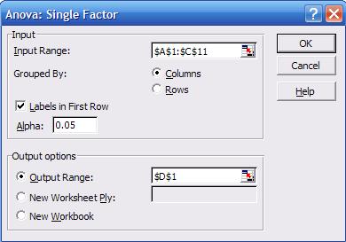
It
looks similar to the one we got when we obtained
«descriptive statistics». Select the input range, check «labels in First Row»,
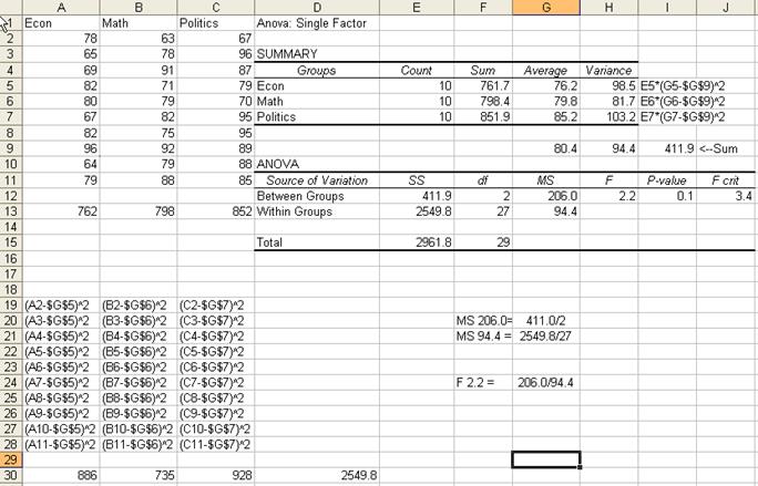
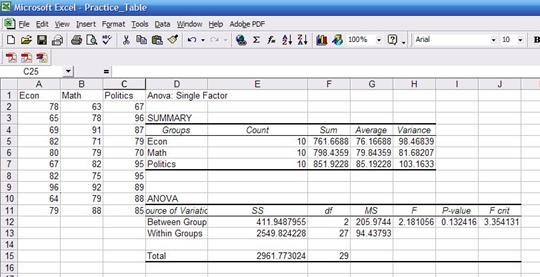
and select as output range «D1», click OK. You»ll get the following:

By
now you should be familiar with the summary statistics presented in the first
table. You may notice that the «sum» column has decimals while the data seems
to be integers. The sum has decimals because some of the scores have decimals;
they are just rounded to the nearest integer.

In
the ANOVA table:

·        
Sources
of variation. The
analysis of variance requires the estimation of two variances: between groups
(econ, math and politics) and the within groups (students).

·        
SS. Sum of square deviations

·        
df.
Degrees of freedom. For between groups is 2 (number of majors minus 1) and for
within groups is 27 (number of students minus number of majors).

·        
MS. Mean square of deviations (variance
estimates), which is equal to SS/df, Roughly 411/2
and 2549/27.

·        
F. Is a probability distribution.
It  is the ratio of two variances.
Roughly 205/94=2.18. According to Kachigan, the F is
the ratio of:

·        
P-value. This is the value that answers your
question. We wanted to know whether there is some sort of relationship between
majors and grades. ANOVA assumes by default that there is no relationship. As a
general rule, a p-value greater than 0.05 means ANOVA»s assumption may be
right. We got a p-value of 0.13 which is greater than 0.05, so it seems there
is no relation between a student»s major and his/her final grade. Had the
p-value been lower than 0.05 then we would have found some kind of relationship
between majors and grades.

·        
F-crit. It is the critical value to check
whether we reject of fail to reject ANOVA»s assumption. Check the table for
0.05 confidence at http://www.statsoft.com/textbook/sttable.html#f05

Here
is a general overview on how some numbers were estimated. Follow the
coordinates by columns and rows

STATA

Stata
is a statistical package to help you perform data analysis, data manipulation
and graphics.

To
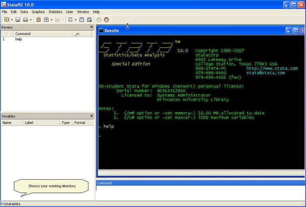
open Stata go to Start — Programs — Stata[ver.*] — Stata[*]. For cluster
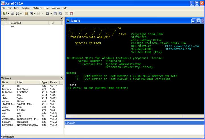
computers contact OIT for instructions. When you open Stata this is what you
will see:

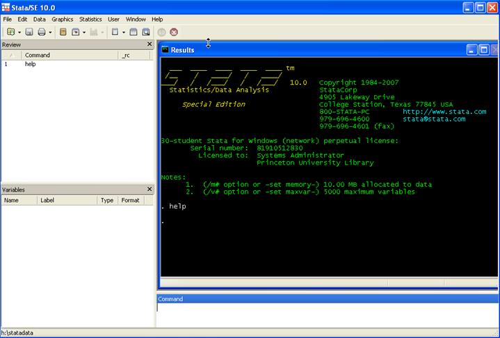
Here
are some brief explanations.

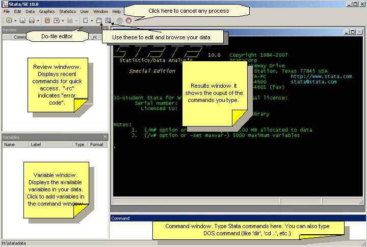
You can
always use the «point-and-click» method by using the menu. We recommend
however, for most of the procedures, to use the command line.

When you work
with Stata there are three basic procedures you may want to do first: create
a log file, set your working directory, and set the correct
memory allocation for your data)

The
log file records everything you type and get while working in Stata. Commands
and output are send to a text file for you to review later. Think of it as a
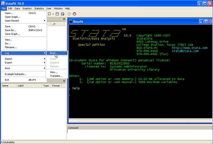
«tape recorder» for your Stata session. To create a log file go
to File — Log — Begin

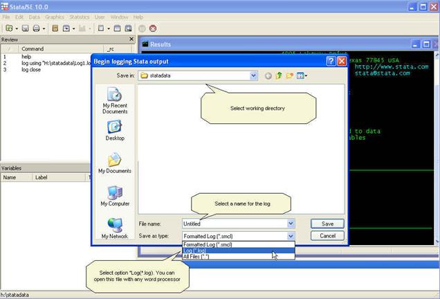
Select
the working directory. In this case will be H:statdata. Name the log and
select the type «Log (*.log)».

In
the results window you will something like

The second
thing to check is your working directory. To do this in the command window type
the following

pwd

Which stands
for «print working directory». This will show you your working directory, which
right now, in this example is H:statadata.

To see what
is in that directory (good old DOS command). Type

dir

For the
purposes of this course we will work in the following directory

H:statadata

To change
directory type in the command window

cd H:statadata

You can check
your current directory by looking at the lower left of the Stata screen.

The third
initial step is to set the necessary memory allocation. In the picture above
you can see in green letters after «Notes:» that the memory allocation is 10 mb. This will be enough for a medium size database but
sometimes you may need more memory space to store your dataset. To determine
the size of your dataset follow the formula:

Size (in
bytes) = (8*Number of cases or rows*(Number of variables + 8))

Depending on your
Stata version and computer power, you can allocate up to around 2 gigabytes. To
allocate 1 g you can type:

set mem 1g

From Excel to
Stata

To
put Excel data to Stata you can simply copy-and-paste.

NOTE: Not recommended for really big
datasets or datasets with long string variables and lots of special characters
(like «;»,»,»,»#»,»%», etc.)

Got
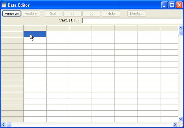
to Stata, click on the «Data editor» icon

A
new window will pop-up, is the data editor window where you can input data or
simply paste it.

In
Excel, select the whole table (A1:N31). Press Ctrl-C. Go to the «Data Editor»
in Stata and paste the table (Ctrl-V)

Numbers
are always black. Red indicates error, in the editor»s case indicates that
values are not numbers, in this case letters or string characters. Close the
data editor by clicking on the «X» in the upper right corner

The
variable window will be populated with all the variables in your data

Stata
automatically eliminates the space in your original titles but keep the format
in the «Label» column. «Type» refers to whether the data is number or string (str*). «Format» shows the length of the variable. In the
command window type help format for
details.

The
whole screen will look like this

Descriptive
statistics

To
start exploring the data you may want to know how many
graduates and undergraduates are in the sample. For this type in the command
window (type help tab for more details):

Click here to
get the data

tab studentstatus

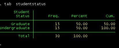
We
have 15 undergrads and 15 grads.

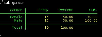
How
many females/males?

tab gender

How
many are econ/politics/math major?

tab major

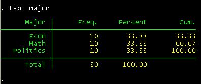
From
what country?

tab country

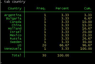
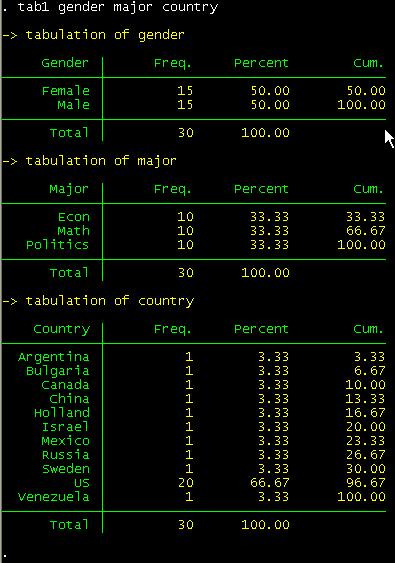
If
you want to run frequencies for more than one variable at the same time use tab1 not tab.

tab1 gender major country

You
should get something like this:

If you want
do a crosstabulation you type:

tab major gender

This is

tab [variable by rows] [variable by column]

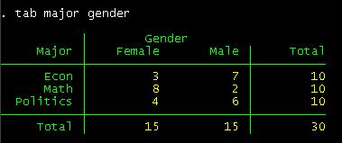
Crosstabulation shows you the subgroups formed by two
variables. You can see that in the sample there are 10 econ majors 3 of which
are females and 7 males. You could also say that there are 15 males 7 of which
are econ major, 2 math and 6 politics.

If you want
percentages by major instead of counts type:

tab major gender, row nofreq

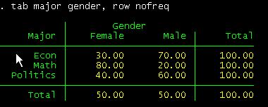
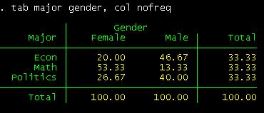
Or by column:

tab major gender, col nofreq

To see more
options type help tab in the command window.

To get more
information on your data we will use the commands: describe, summarize, tabstat and a combination of tab and summarize.

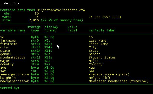
In the
command window type describe.
The describe command will provide you info for the
active dataset and the format of the variables («display format»). [Hit enter
or spacebar to see the rest of the list]. Type help describe for further details (if the «—more—
» message bugs you, type set
more off)

Summarize will provide you with some familiar
descriptive statistics.

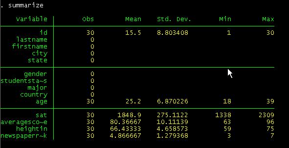
If
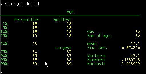
you type summarize, detail, you will get a more detail set of statistics (press
bar space to continue)

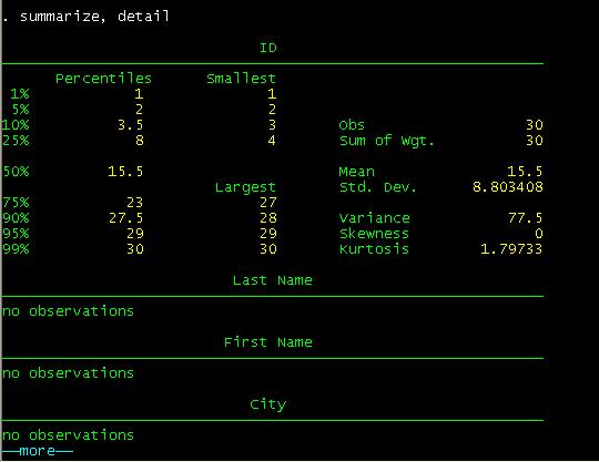
We
skip some results to accommodate some in one window.

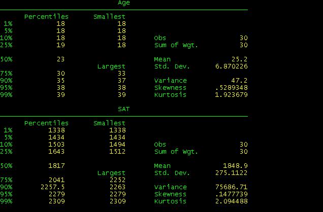
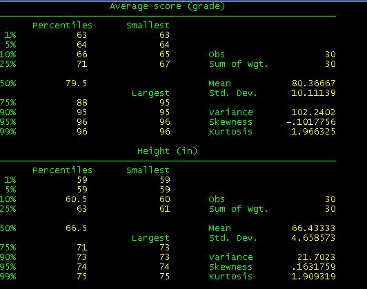
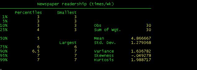
When
you compare these results with the excel file you will see they are basically
the same with the exception of Skewness and Kurtosis which Stata calculates
differently.

Tabstat is another command that provide
summary statistics

In
the command line type. To fastrack type tabstat and then click on each variable in the variables windowo. The «s» before the parenthesis stands for
«statistics» here you select the statistics you need.

tabstat    age sat averagescoregrade heightin newspaperreadershiptimeswk, s(mean semean
median sd var skew k count
sum range min max )

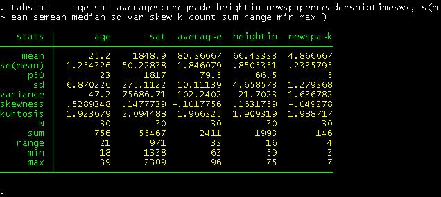
This
table looks similar to the one obtained in excel. Notice that «p50» is the
median.

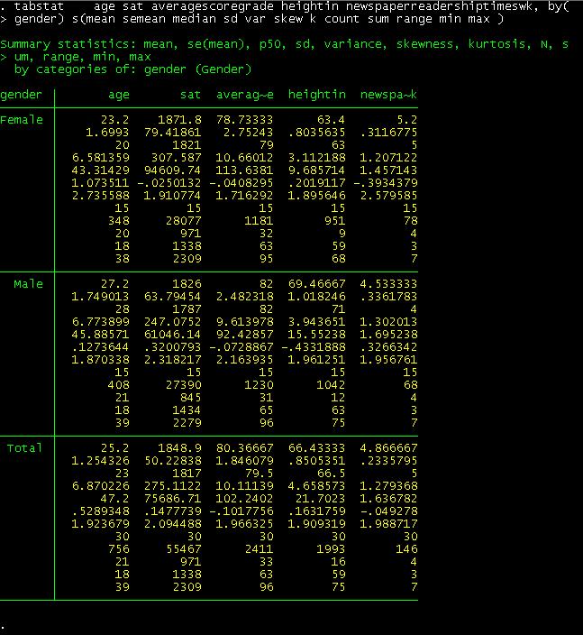
If
you are interested in getting these statistics by gender just add after the
comma the option by(gender)

To
recreate the pivot table we did in excel we just type the
following:

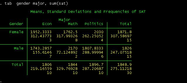
This
is a crosstab between gender and student»s major regarding SAT»s scores. The
following part provide us the way to read the table

For
example, for the cross between females and Econ. A female student with an econ
major has an average SAT score of 1952, with a standard deviation of 312 and in
the sample there are only three students in this category.

Without
the option sum(sat), we will get a simple crosstabulation
between gender and major

You
can have more options if you want (type help
tab for details). For
example if you want percentage by columns and row type:

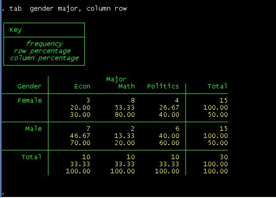
You
can read this table as follows. Among female students, 20% are econ major,
53.3% are math and 26.67% are in politics.

Among
econ majors, 30% are females and 70% are males.

Let»s
say you wan only column percents,
type

tab gender major, column nofreq

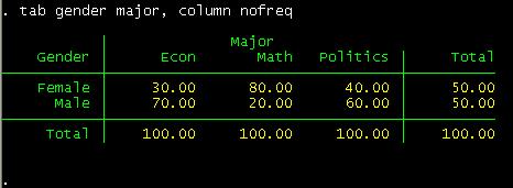
Notice
the «nofreq» option.

By the way, remember the little warm-up we had in excel
converting last and first names into proper format? Well, we can do that in
Stata as well. The following introduces a way to generate new variables (type help generate for more details)

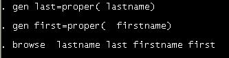
When
you hit enter after browse you will see the
difference.

Rolling standard deviation

*******If you do not see
the menu on the left click
here to see it

NOTE: Replace words in italics with your own

This
will produce a rolling standard deviation every three years as indicated in the
option window()
below, adjust it to your desired window:

cd H:
use http://dss.princeton.edu/training/Panel101.dta,
clear

xtset country year
rolling x1_sd=r(sd),
window(3) saving(x1_sd): sum x1
use x1_sd
rename end year
save, replace
use http://dss.princeton.edu/training/Panel101.dta,
clear
merge 1:1 country year using x1_sd
drop _merge

For
more details type

help rolling

For
similar commands type

help tssmooth

ANOVA using
Stata

*******If you do not see
the menu on the left click
here to see it

One-way
ANOVA tests whether the mean of the dependent variable (y) is statistically significant among different categories of the
independent variable (x). The format
is

oneway [measurement] [categorical]

In
the example below, we are interested on testing whether a student»s major has
some effect on his/her grade. Type:

oneway averagescoregrade major, tabulate

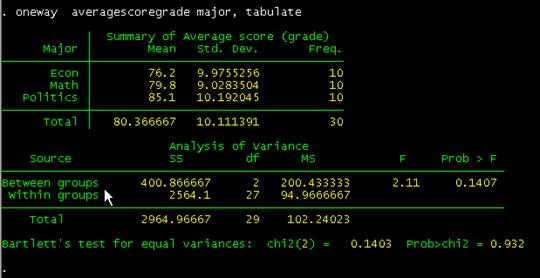
Comparing
these with the results using excel (shown below) they are pretty close. «Prob>F» is the p-value which has to be lower than 0.05
(for 95% confidence) to be significant. Conclusions are basically the same.

For
more details and more options type help
oneway.

As
an exercise run one-way ANOVA by gender.

Graphs

If
you go to the menu and click «Graphics» you will see all the graphing options available
in Stata. If you do not have it already, click
here to get the data to do these graphs.

Let»s
see one basic scatterplot. We will add some options later.
Scatterplots are good to explore possible relationships between variables and
to identify outliers. In this case we want to explore visually whether there is
some relationship between age and SAT scores. If there is some kind of
relationship we would be able to see a specific patter (linear, curve, concave,
etc.). For many more bells and whistles type help scatter
in the command window. The format is twoway scatter y x.
For starters let»s type:

twoway scatter sat age

There
seems to be a downward relationship, older students may show lower SAT scores.
Each dot represents a student, the option mlabel below will help you identify and label the dots.

twoway scatter sat age, mlabel(lastname)

To
fit a regression line type:

twoway scatter
sat age, mlabel(last) || lfit
sat age

You
may want to add some quadrants as in the following.

Quadrants
here represent the mean of both variables. Here is how to do it:

Type

sum age, detail

Then
type:

return list

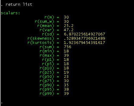
In
this case we are interested in the mean of «age», so we save it as a temporary
variable by typing:

local meanage=r(mean)

We
do the same thing with «sat»

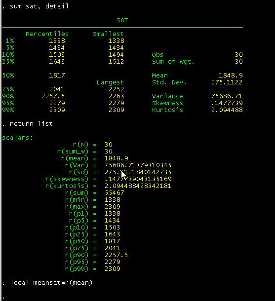
The
local command is used for macros an assigns strings names to macros. In  this case we create temporary variables. To
make the graph with the quadrants type:

twoway scatter
sat age || lfit sat age, yline(`meansat‘) xline(`meanage‘)

Notice
the «yline» and «xline»
options after comma and the single quotes.

If
you want to set your own parameters for the quadrants just type the number in
the «yline» and «xline»
options. For example we want lines that cross age at 30 and SAT at 1800:

twoway scatter sat age, mlabel(lastname) || lfit sat age, yline(1800) xline(30)

If
you want to include the confidence bands we have to reverse the order of the
graphs because the shaded area tends to cover the dots. So we graph the
confidence region first, then the scatter.

twoway (lfitci sat age) || (scatter sat age)

Or
with labels.

twoway (lfitci sat age) || (scatter sat age, mlabel(lastname))

You
may want to add a title to the graph and a title to the y-axis.

twoway (lfitci age sat) || (scatter age sat, mlabel(lastname)), title(«SAT scores by age») ytitle(«Age»)

One
problem in the graph is that some labels overlap making it difficult to read
them.

We
can rearrange them by moving them around the marker in a 12-hour clock
position.

We
need to create the variable position
first. Type:

generate position=3

Position
= 3 is the default, notice that all labels are to the right of the marker (3
pm).

We»ll
move DOE29 to 12 o»clock and DOE10 to 6.

[IMPORTANT: If you get the message «(0
real changes made)» make sure you spell the names correctly, Stata is
case-sensitive.]

To
change the desired positions use the option mlabv()

twoway (lfitci sat age) || (scatter sat age, mlabel(lastname) mlabv(position)),
title(«SAT scores by age») ytitle(«SAT»)

You
may want to see if there is some kind of relationship by particular groups,
let»s say by gender.

twoway scatter sat age, mlabel(lastname) by(gender,
total)

Or
by major,

twoway scatter age sat, mlabel(lastname) by(major, total)
|| lfit age sat

Histogram

Histograms
are another good way to visually explore data, especially to check for a normal
distribution; here are some examples (type help histogram
in the command window for further details):

histogram age, frequency

Adding
a normal curve…

histogram age, frequency normal

Age
by gender

histogram age, frequency by(gender,
total)

A
histogram with SAT scores by gender.

histogram sat, frequency by(gender,
total)

To
save graph right-click on the graph, select «save graph» or you can also copy
it to word by selecting «copy graph».

Bar chart

graph hbar (mean) age  averagescoregrade newspaperreadershiptimeswk, over(gender) over(  studentstatus,
label(labsize(small))) blabel(bar)
title(«Student indicators»)

graph hbar (mean) age  averagescoregrade newspaperreadershiptimeswk, over(gender) over(studentstatus, label(labsize(small)))
blabel(bar) title(Student indicators) legend(label(1
«Age») label(2 «Score») label(3 «Newsp
read»))

Graphing categorical data

To
graph categorical data in Stata you will need a special program called catplot. If your version of Stata does not
have it, you can install it by typing

ssc install catplot

Now
type:

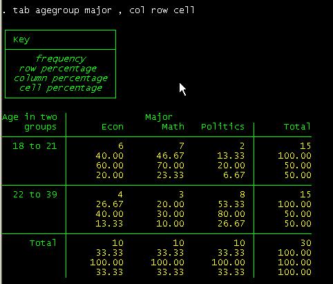
tab agegroup
major, col row cell

To
graph this table type:

catplot bar major agegroup, blabel(bar)

This will get you the following:

Notice you may have to create the variable «agegroup» which is a recode of «age» where 1 «18 to 21» 2
«22 to 39».

The
labels on the graph correspond to the number of students on each group. For
example there are 6 students econ majors with ages between 18 to 21.

If
you are interested on the percentages within «agregroup»
you can specify this as follows:

catplot  bar major agegroup,
percent(agegroup) 
blabel(bar)

The
percent() option indicates the reference group
displayed in the graph. The labels on the previous graph correspond to the
second row in the crosstab between agegroup and
major.

If
you are interested on the percentages within «major» you can specify this as
follows:

catplot  bar agegroup major,
percent(major)  blabel(bar)

References
and useful links

Hamilton,
Lawrence C.Statistics with Stata (updated
for Version 9). Brooks/Cole, 2006

Kachigan, Sam, Statistical analysis: an interdisciplinary introduction to univariate
& multivariate methods. New
York : Radius Press, c1986.

Textbook Examples.
Regression with Graphics. by Lawrence Hamilton

http://www.ats.ucla.edu/stat/examples/rwg/

Stata Library. Graph
Examples (may not work with STATA 10)

http://www.ats.ucla.edu/STAT/stata/library/GraphExamples/default.htm

DSS
help-sheets for STATA

http://dss/online_help/stats_packages/stata/stata.htm

Introduction
to Stata (PDF),
Christopher F. Baum, Boston College,
USA

A 67-page
description of Stata, its key features and benefits, and other useful
information.

http://fmwww.bc.edu/GStat/docs/StataIntro.pdf

STATA
Corporation»s links to resources for learning STATA

http://stata.com/links/resources1.html

STATA FAQ website

http://stata.com/support/faqs/

Useful links
to data, software and analysis

http://www.princeton.edu/~otorres/

UCLA
Resources to learn and use STATA

http://www.ats.ucla.edu/stat/stata/

Graphs in
Stata

http://data.princeton.edu/stata/Graphics.html