
Excel for Microsoft 365 Excel for Microsoft 365 for Mac Excel for the web Excel 2021 Excel 2021 for Mac Excel 2019 Excel 2019 for Mac Excel 2016 Excel 2016 for Mac Excel 2013 Excel 2010 Excel 2007 Excel for Mac 2011 Excel Starter 2010 More…Less
Important: The calculated results of formulas and some Excel worksheet functions may differ slightly between a Windows PC using x86 or x86-64 architecture and a Windows RT PC using ARM architecture. Learn more about the differences.
Click one of the links in the following list to see detailed help about the function.
|
Function |
Description |
|
DAVERAGE function |
Returns the average of selected database entries |
|
DCOUNT function |
Counts the cells that contain numbers in a database |
|
DCOUNTA function |
Counts nonblank cells in a database |
|
DGET function |
Extracts from a database a single record that matches the specified criteria |
|
DMAX function |
Returns the maximum value from selected database entries |
|
DMIN function |
Returns the minimum value from selected database entries |
|
DPRODUCT function |
Multiplies the values in a particular field of records that match the criteria in a database |
|
DSTDEV function |
Estimates the standard deviation based on a sample of selected database entries |
|
DSTDEVP function |
Calculates the standard deviation based on the entire population of selected database entries |
|
DSUM function |
Adds the numbers in the field column of records in the database that match the criteria |
|
DVAR function |
Estimates variance based on a sample from selected database entries |
|
DVARP function |
Calculates variance based on the entire population of selected database entries |
Need more help?
Database Function in Excel (Table of Contents)
- Introduction to Database Function in Excel
- How to Use Database Function in Excel?
Introduction to Database Function in Excel
Excel database functions are designed in such a way that a user can use an Excel database to perform the basic operation on it like Sum, Average, Count, Deviation, etc. The database function is an in-built function in MS Excel that will work only on the proper database or table. These functions can be used with some criteria also.
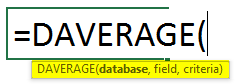
Syntax:
There are some specific in-built Database Functions which are listed below:
- DAVERAGE: It will return the average of the selected database, which is satisfying the user criteria.
- DCOUNT: It will count the cells containing some number in the selected database and satisfy the user criteria.
- DCOUNTA: It will count the non-blank cells in the selected database and which is satisfying the user criteria.
- DGET: It will return a single value from the selected database, which is satisfying the user criteria.
- DMAX: It will return the maximum value of the selected database, which is satisfying the user criteria.
- DMIN: It will return the minimum value of the selected database, which is satisfying the user criteria.
- DPRODUCT: It will return the multiplication output of the selected database, which is satisfying the user criteria.
- DSTDEV: It will return the estimated standard deviation of the population based on the entire population in the selected database, which is satisfying the user criteria.
- DSTDEVP: It will return the standard deviation of the entire population based on the selected database, which is satisfying the user criteria.
- DSUM: It will return the summation of the value from the selected database, which is satisfying the user criteria.
- DVAR: It will return the estimated variance of the population based on the entire population in the selected database, which is satisfying the user criteria.
- DVARP: It will return the Estimates variance of the entire population in the selected database, which is satisfying the user criteria.
How to Use Database Functions in Excel?
Database Functions in Excel is very simple and easy. Let’s understand how to use the Database Functions in Excel with some examples.
You can download this Database Function Excel Template here – Database Function Excel Template
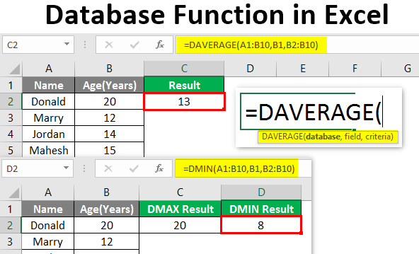
Example #1 – Using DAVERAGE Database Function in Excel
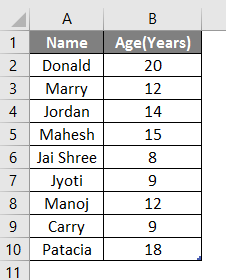
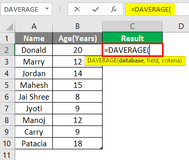
Let’s assume a user has some people’s personal data like Name and Age, where the user wants to calculate the average age of the people in the database. Let’s see how we can do this with the DAVERAGE function.
Open MS Excel from the Start menu, Go to Sheet where the user has kept the data.
Now create headers for DAVERAGE result where we will calculate the average of the people.
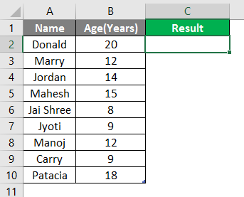
Now calculate the DAVERAGE of the given data by DAVERAGE function, use the equal sign to calculate, Write in C2 Cell.
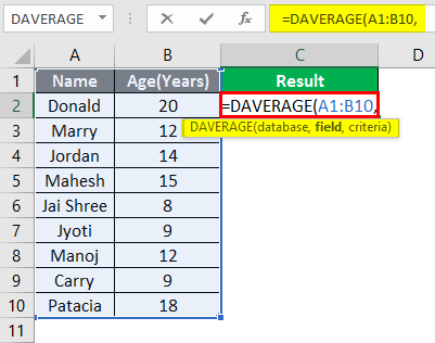
It will then ask for the database given in A1 to B10 cell, select A1 to B10 cell.
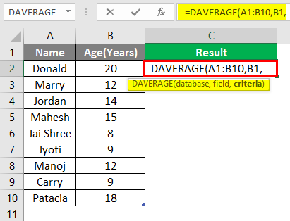
Now it will ask for the Age, so select C1 cell.
It will then ask for criteria from B2 to B10 cell where the condition will be applied and select B2 to B10 cell.
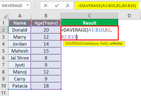
Press the Enter Key.
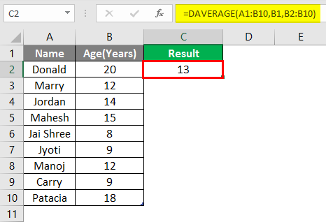
Summary of Example 1: As the user wants to calculate the average age of the people in the database. Everything is calculated in the above excel example, and the Average age is 13 for the group.
Example #2 – Use of DMAX and DMIN Database Function in Excel
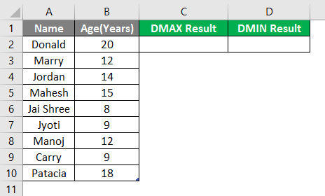
Let’s assume a user has few personal data, like Name and Age, where the user wants to find out the maximum and minimum age of the people in the database. Let’s see how we can do this with the DMAX and DMIN function. Open MS Excel from the Start menu, Go to Sheet where the user kept the data.
Now create headers for DMAX and DMIN results where we will calculate the maximum and minimum age of the people.
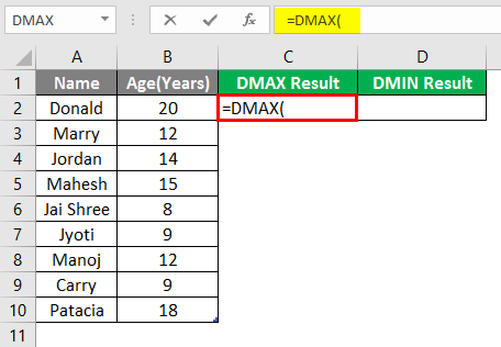
Now calculate the maximum age in the given age data by DMAX function, use the equal sign to calculate, Write in a formula in cell C2.
It will then ask for the database given in cell A1 to B10 and select cell A1 to B10.
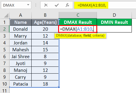
Now it will ask for Age, select B1 cell.
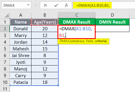
Now it will ask for criteria which are cells B2 to B10 where the condition will be applied, select cell B2 to B10.
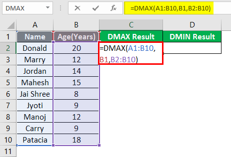
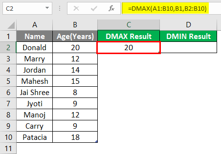
Press the Enter Key.
Now to find out the minimum age, use the DMAX function and follow steps 4 to 7. Use the DMIN formula.
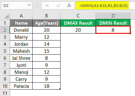
Summary of Example 2: As the user wants to find out the maximum and minimum age of the people in the database. Easley everything calculated in the above excel example and the Maximum age is 20, and the minimum is 8 for the group.
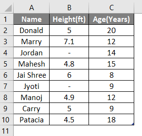
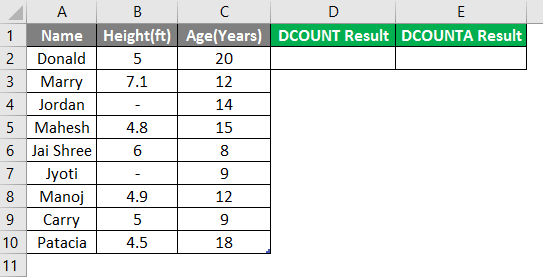
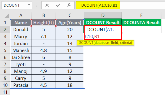
Example #3 – Use of DCOUNT and DCOUNTA Database Function in Excel
A user wants to find out the numeric data count and nonblank cell count in the height column in the database. Let’s see how we can do this with the DCOUNT and DCOUNTA function. Open MS Excel from the Start menu; go to Sheet3, where the user kept the data.
Now create headers for DCOUNT and DCOUNTA results.
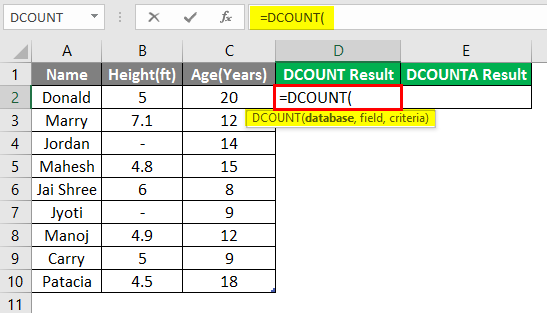
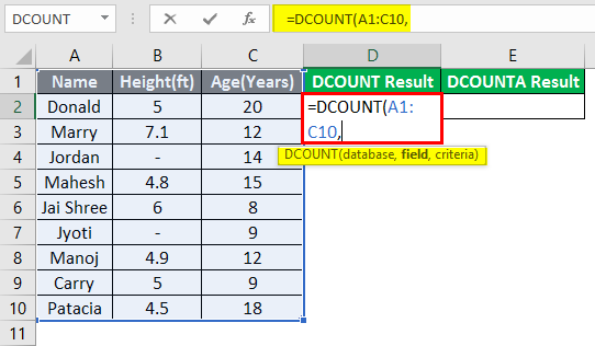
Write the formula in cell D2.
It will then ask for the database given in cell A1 to C10 and select cell A1 to C10.
Now it will ask for the Height, select cell B1.
Now it will ask for criteria which are cell B2 to B10, where the condition will be applied, select cell B2 to B10.
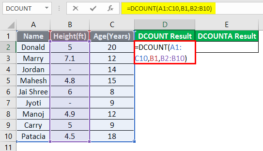
Press Enter key.
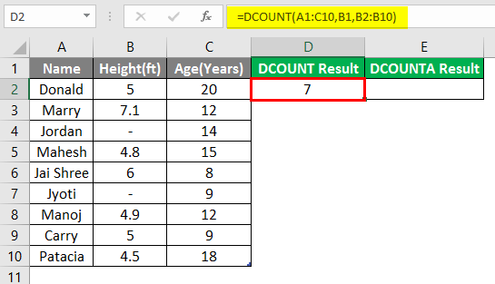
Now to find out nonblank cell function follow steps 4 to 7. Use the DCOUNTA formula.
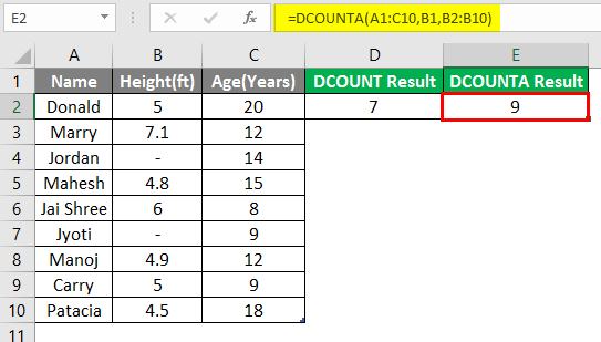
Summary of Example 3: As the user wants to find out the numeric data count and nonblank cell count in the height column. Easley everything calculated in the above excel example, the numeric data count is 7, and the nonblank cell count is 9.
Things to Remember About Database Functions in Excel
- All database functions follow the same syntax, and it has 3 arguments: a database, field, and criteria.
- Database function will work only if the database has a proper table format like it should have a header.
Recommended Articles
This is a guide to Database Function in Excel. Here we discuss how to use Database Function in Excel along with practical examples and downloadable excel template. You can also go through our other suggested articles –
- Excel Create Database
- Excel Database Template
- User-Defined Function in Excel
- PRODUCT Function in Excel
Database functions are designed to perform simple operations on data that is in a “database-like structure”. Database-like structure means that the data must be in a table structure that has organized records with labels and appropriate separation. In this model, each row represents an individual record, and each column is a different type of information. For data that is in this structure, you can use Excel database functions to manipulate and manage your tables much more efficiently.
Excel Database Functions Overview
All Excel database functions, except for DGET, can be used just like the xIFS functions (SUMIFS, AVERAGEIFS, etc.). xIFS formulas perform the specific aggregation or operation on a certain column, with specified filters. On the other hand, the DGET function can grab a cell value as is, without any aggregation, if there is only a single result after filters are applied. Below is a list of Excel database functions.
| Function | Description |
| DAVERAGE | Returns the average of selected database entries |
| DCOUNT | Counts the cells that contain numbers in a database |
| DCOUNTA | Counts nonblank cells in a database |
| DGET | Extracts from a database a single record that matches the specified criteria |
| DMAX | Returns the maximum value from selected database entries |
| DMIN | Returns the minimum value from selected database entries |
| DPRODUCT | Multiplies the values in a particular field of records that match the criteria in a database |
| DSTDEV | Estimates the standard deviation based on a sample of selected database entries |
| DSTDEVP | Calculates the standard deviation based on the entire population of selected database entries |
| DSUM | Adds the numbers in the field column of records in the database that match the criteria |
| DVAR | Estimates variance based on a sample from selected database entries |
| DVARP | Calculates variance based on the entire population of selected database entries |
The formulas look and work very much like their IFS counterparts, the only exception being the DGET function.
Syntax
All Excel database functions use the same syntax which has 3 arguments for data, field, and filters. All arguments are required.
| Database | The range of cells containing the data itself. The top row of the range contains labels for each column. |
| Field | The column that is to be used in calculations. A label (name) or position of a column can be entered. You can enter a name inside quotation marks, such as «Base Salary», or a position index, such as 7 for the 7th column. |
| Criteria | The range of cells that contain the conditions that will determine which records are to be included in the calculations. Criteria has label of column(s) to be filtered and condition(s) under the label. |

Building a criteria
Building the criteria logic might seem intimidating at first. You can create conditions and join them using AND and OR logical operators. The idea is that every condition inside a row is connected with an AND logic, whereas every row is connected with an OR. Let’s see these logical statements in examples. Feel free to download our sample workbook below.
Basics
Enter the field names (columns) in a single row, where you would like to add to the criteria. For example, if we want to filter Atlanta values in a column named Location, our criteria should be like below.

If we need to add a second value for Location, the second value should be placed under the first one. Below criteria refers to the records that has Atlanta or Valdosta values in the corresponding Location. This is an OR connection.

Alternatively, if we want to get records that have Atlanta for Location AND Year smaller than 2017, we need to use the same row.

Note that you can use <, >, <=, >= and <> operators as well. Although, Excel suggests using = with equal conditions, this is not mandatory. The database formulas support * and ? wildcards for unknown characters. To learn more about wildcard characters in Excel, please see How to use a wildcard in Excel formula.
Complex Examples
Multiple AND logic
Boolean logic: (Location = Atlanta AND Year > 2011 AND Year < 2018)
Records in Atlanta between 2011 and 2018.

Multiple OR statements
Boolean logic: (Location = Atlanta OR Location = Dothan OR Location = Valdosta)
Records in Atlanta or Dothan or Valdosta.

OR logic between different fields
Boolean logic: (Location = Atlanta OR Department <> R&D)
Records in Atlanta or not in R&D department.

You can leave fields empty when you do not need them in the criteria.
Combination of AND or OR logics
Boolean logic: ( (Location = Atlanta AND Year > 2011 AND Year < 2018) OR (Location = Dothan AND Department <> R&D) )
Records in Atlanta between 2011 and 2018, or in Dothan but not in R&D department.

Wildcards
Boolean logic: (Full Name = Dana* AND Location = Atlanta AND Year = 2018)
Records with names starting with Dana in Atlanta and in 2018. The department is irrelevant in this case.

Advantages & Disadvantages
Once you understand the structural requirements, managing data in a database-like structure becomes much easier. Finally, let’s take a quick look at some of the advantages and disadvantages of using Excel database formulas, instead of traditional aggregation methods.
Advantages
- Easy to create and modify filters and target column without updating formulas.
- Easy to manage complex filters.
- A single named range is enough in most cases.
- Supports AND and OR logic checks (xIFS functions only supports AND).
Disadvantages
- Data must have headers
- Slight learning curve
Содержание
- How to Use Database Functions in Excel
- General Syntax
- DAVERAGE
- DCOUNT
- DCOUNTA
- DPRODUCT
- DSTDEV
- DSTDEVP
- Creating a database in Excel and its functionality
- Step by step to create a database in Excel
- Excel functions for working with database
- Working with databases in Excel
- Data sorting
- Sort by condition
- Subtotals
How to Use Database Functions in Excel
In this lesson, you will learn about all the database functions in Excel.
Database functions are used to analyze data stored in a database. They have a few common features:
- Each function has three parameters: database, field and criteria. These parameters indicate the worksheet area used by the function.
- Except for the GETPIVOTDATA function, the other twelve functions start with the letter D.
- If you remove the letter D, you may notice that most of the database functions have already appeared in other types of functions in Excel. For example, if from DAVERAGE you remove D, this is well-known AVERAGE function.
General Syntax
Function_name (database, field, criteria)
- Database – range of cells, where your database is
- Field – name or numer of column where values are
- Criteria – your criteria should contain the name of the column and the name of some value from that column.
Let’s train that with examples. To use a database function in Excel, you’ll first need to set up your data in a format that Excel recognizes as a database. This typically involves organizing your data into columns and rows, and using headings for each column. This is an example database:
DAVERAGE
This function shows the average of values that meet your criteria.
The syntax for the DAVERAGE function is:
DAVERAGE(database, field, criteria)
- «database» is the range of cells that make up your database, such as «A1:C10».
- «field» is the column number that you want to average. For example, if you want to average values from column 2, you would enter «2».
- «criteria» is the conditions that must be met for a cell to be included in the calculation. For example, you might use «A2:A10 = «Apples» to average only the values in column 2 that correspond to the «Apples» in column 1.
This is an example:
=DAVERAGE($A$1:$C$11;3;$A$1:$A$2) or =DAVERAGE($A$1:$C$11;»Sales»;$A$1:$A$2)
Note that the DAVERAGE function will only average cells that contain numbers. If a cell in the specified field contains text or an error value, that cell will be ignored in the calculation.
DCOUNT
This function shows the count of cells that meet your criteria.
The syntax for the DCOUNT function is:
DCOUNT(database, field, criteria)
- «database» is the range of cells that make up your database, such as «A1:C10».
- «field» is the column number that you want to count. For example, if you want to count values from column 2, you would enter «2».
- «criteria» is the conditions that must be met for a cell to be included in the calculation. For example, you might use «A2:A10 = «Apples» to count only the values in column 2 that correspond to the «Apples» in column 1.
This is an example:
=DCOUNT($A$1:$C$11,3,$E$2:$E$3) or =DCOUNT($A$1:$C$11,»Sales»,$E$2:$E$3)
DCOUNTA
This function shows the number of noblank cells that meet your criteria. The DCOUNTA function works similarly to the DCOUNT function.
The syntax for the DCOUNTA function is:
DCOUNTA(database, field, criteria)
- «database» is the range of cells that make up your database, such as «A1:C10».
- «field» is the column number that you want to count. For example, if you want to count values from column 2, you would enter «2».
- «criteria» is the conditions that must be met for a cell to be included in the calculation. For example, you might use «A2:A10 = «Apples» to count only the values in column 2 that correspond to the «Apples» in column 1.
This is an example:
=DCOUNTA($A$1:$C$11,3,$E$2:$E$3) or =DCOUNTA($A$1:$C$11,»Sales»,$E$2:$E$3)
Note that the DCOUNTA function will count all cells in the specified field, including cells that contain text, numbers, and error values.
This function shows a single value that meets your criteria.
The function has the following syntax:
DGET(database, field, criteria)
- database: The range of cells that makes up the database. The first row of the range should contain the column labels.
- field: The column label that you want to retrieve the data from.
- criteria: A range of cells that contains the conditions you want to apply to the database. The first row of the criteria range should contain the column labels that correspond to the database.
This is an example:
=DGET($A$1:$C$11,3,A1:A2) or =DGET($A$1:$C$11,»Sales»,A1:A2)
If the criteria match multiple rows in the database, the DGET function will return only the first match it finds.
This function shows the max value that meets your criteria.
The function has the following syntax:
DMAX(database, field, criteria)
- database: The range of cells that makes up the database. The first row of the range should contain the column labels.
- field: The column label that you want to find the maximum value in.
- criteria: A range of cells that contains the conditions you want to apply to the database. The first row of the criteria range should contain the column labels that correspond to the database.
This is an example:
=DMAX($A$1:$C$11,3,$A$1:$A$2) or =DMAX($A$1:$C$11,»Sales»,$A$1:$A$2)
The DMAX function only returns the maximum value from a single column, not the entire row. If multiple rows in the database meet the criteria, the DMAX function will return the maximum value from the specified field for all matching rows.
This function shows the min value that meets your criteria.
The function has the following syntax:
DMIN(database, field, criteria)
- database: The range of cells that makes up the database. The first row of the range should contain the column labels.
- field: The column label that you want to find the minimum value in.
- criteria: A range of cells that contains the conditions you want to apply to the database. The first row of the criteria range should contain the column labels that correspond to the database.
This is an example:
=DMIN($A$1:$C$11,3,$A$1:$A$2) or =DMIN($A$1:$C$11,»Sales»,$A$1:$A$2)
The DMIN function only returns the minimum value from a single column, not the entire row. If multiple rows in the database meet the criteria, the DMIN function will return the minimum value from the specified field for all matching rows.
DPRODUCT
This function shows the multiplication of values that meet your criteria.
The function has the following syntax:
DPRODUCT(database, field, criteria)
- database: The range of cells that makes up the database. The first row of the range should contain the column labels.
- field: The column label that you want to calculate the product of.
- criteria: A range of cells that contains the conditions you want to apply to the database. The first row of the criteria range should contain the column labels that correspond to the database.
This is an example:
=DPRODUCT($A$1:$C$11,3,$A$1:$A$2) or =DPRODUCT($A$1:$C$11,»Sales»,$A$1:$A$2)
If multiple rows in the database meet the criteria, the DPRODUCT function will return the product of the specified field for all matching rows. The DPRODUCT function only works with numeric values, and it will return an error if any of the cells in the specified field contain text or empty cells.
DSTDEV
This function estimates the standard deviation of values that meet your criteria.
The function has the following syntax:
DSTDEV(database, field, criteria)
- database: The range of cells that makes up the database. The first row of the range should contain the column labels.
- field: The column label that you want to calculate the standard deviation of.
- criteria: A range of cells that contains the conditions you want to apply to the database. The first row of the criteria range should contain the column labels that correspond to the database.
This is an example:
=DSTDEV($A$1:$C$11,3,$A$1:$A$2) or =DSTDEV($A$1:$C$11,»Sales»,$A$1:$A$2)
If multiple rows in the database meet the criteria, the DSTDEV function will return the standard deviation of the specified field for all matching rows. The DSTDEV function only works with numeric values, and it will return an error if any of the cells in the specified field contain text or empty cells.
DSTDEVP
This function estimates standard deviation based on the whole population of values that meet your criteria.
It uses the following syntax:
DSTDEVP(database, field, criteria)
- database: is the range of cells that makes up the list or database.
- field: is the column in the database that you want to base your calculations on. This argument should be a number that represents the column number.
- criteria: is an optional argument that allows you to specify certain conditions or criteria that the data in the field must meet in order to be included in the calculation.
This is an example:
=DSTDEVP($A$1:$C$11,3,$A$1:$A$2) or =DSTDEVP($A$1:$C$11,»Sales»,$A$1:$A$2)
This function shows the sum of values that meet your criteria.
The syntax for the DSUM function is as follows:
DSUM(database, field, criteria)
- database: is the range of cells that makes up the list or database.
- field: is the column in the database that you want to base your calculations on. This argument should be a number that represents the column number.
- criteria: is an optional argument that allows you to specify certain conditions or criteria that the data in the field must meet in order to be included in the calculation.
This is an example:
=DSUM($A$1:$C$11,3,$A$1:$A$2) or =DSUM($A$1:$C$11,»Sales»,$A$1:$A$2)
The DSUM function only works with lists or databases that have column headers. If your database does not have column headers, you should use a different function, such as SUMIF.
This function estimates the variance of values that meet your criteria.
The syntax for the DVAR function is as follows:
DVAR(database, field, criteria)
- database: is the range of cells that makes up the list or database.
- field: is the column in the database that you want to base your calculations on. This argument should be a number that represents the column number.
- criteria: is an optional argument that allows you to specify certain conditions or criteria that the data in the field must meet in order to be included in the calculation.
This is an example:
=DVAR($A$1:$C$11,3,$A$1:$A$2) or =DVAR($A$1:$C$11,»Sales»,$A$1:$A$2)
This function estimates the variance of values that meet your criteria based on the entire population.
The syntax for the DVARP function is as follows:
DVARP(database, field, criteria)
- database: is the range of cells that makes up the list or database.
- field: is the column in the database that you want to base your calculations on. This argument should be a number that represents the column number.
- criteria: is an optional argument that allows you to specify certain conditions or criteria that the data in the field must meet in order to be included in the calculation.
This is an example:
=DVARP($A$1:$C$11,3,$A$1:$A$2) or =DVARP($A$1:$C$11,»Sales»,$A$1:$A$2)
Источник
Creating a database in Excel and its functionality
Any database (DB) is a summary table with the parameters and information. Most schools programs included the creation of a database in Microsoft Access. But Excel gives all the opportunities to build simple databases and easily navigate through them.
How to make the database in Excel so it was convenient not to only store but also process the data: generate reports, build charts, graphs, etc.
Step by step to create a database in Excel
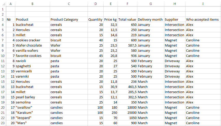
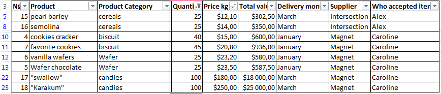
At first we will learn how to create a database using Excel tools. Let’s imagine that we are the shop. We draw up a summary table of data with various products deliveries from different suppliers.
| № | Product | Product Category | Quantity | Price kg | Total value | Delivery month | Supplier | Who accepted items |
We puzzled out with headlines. Now fill the table. We start with a serial number. We don’t have to put down the numbers manually. Enter in cells A4 and A5 one and two respectively. Then select those two cells with left mouse button and grab the corner of the segregation and extend down to any number of rows. In a small little window you will see the final number.
Note. This table can be downloaded at the end of the article.
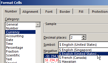
Base show us that some of the information will be presented in text form (product, category, month, etc.), and some is in the financial. Select the cells with the headlines named Price kg and Total value E4:F23. Use right-click to see context menu where choose «Format Cells» CTRL+1.
A window will appear where we will choose the Currency format. Enter the number of decimal places equals 1. We don’t have to choose designation because in the header we already pointed out that the price and value in $ English (United States).
Similarly we proceed with the cells where the quantity column will be filled. Select numerical number.
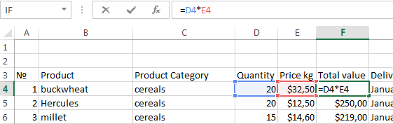
Let’s deal with another preparatory action. You can immediately use that fact that in the corresponding cells value is calculated as the price multiplied by the quantity. To make this we enter in cell F4 formula and stretch it to the other cells in this column. Thus the cost will be calculated automatically while filling the table.
Now fill the table with data.
It’s important! It is necessary to stick to a single style of writing while filling the cells. If the original name of the employee is recorded as Alex AA, then the rest cells should be filled similarly. The work with the database will be difficult if somewhere name will be written differently, for example, Alexey Alex.
The table is ready. In reality it may be much longer. We have added a several positions for example. Let us give the database a more aesthetic appearance with making the frame. To do this select the entire table and find the parameter «All Borders» on the panel.
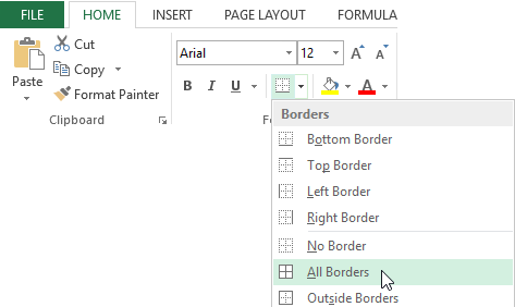
Similarly, frame the headlines thick outer boundary.
Excel functions for working with database
Now we turn to the functions that Excel offers to work with the database.
Working with databases in Excel
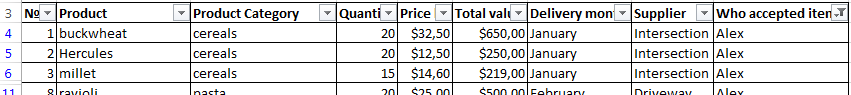
Example: we want to know all the products receipted by Alex AA Theoretically, you can run through the all rows visually where this name appears and then copy them to a separate table. But what if our database composed of several hundreds of items? FILTER comes to help us.
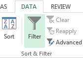
Select all the headlines in the table and click «FILTER» in the «DATA» tab, (CTRL + SHIFT + L).
In each cell in the header appears black arrow on a gray background which can be clicked to filter the data. Click it in the parameter WHO ACCEPTED ITEMS and remove the check mark from the CAROLINE name.
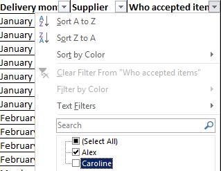
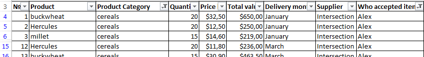
Thus there are remains data only with Alex.
Note! When you are sorting data not only all the positions in the columns stays in its places but rows of numbers also corresponding to the sheet (these are highlighted in blue). This feature is useful to us later.
You can make additional filtering. Determine which kind of grouts Alex accepted. Click the arrow on the cell PRODUCT CATEGORIY and leave only grouts.
If you need to return the full database you can make it in easiest way: set out all the checkboxes in the corresponding filters.
Data sorting
In this example the database was filled in chronological order during the supplying goods in the shop. But if we want to sort the data on a different principle excel allows you to do that too.
For example, we want to sort the products as price increase. Those the first line will be the cheapest product and in the last will be the most expensive. Select the column with the price and on the HOME tab and choose the «Sort & Filter».
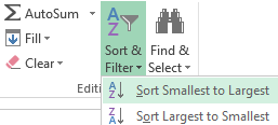
As we decided that lower price would be on top choose «Sort Smallest to Largest». You will see another window where we select «Expand the selection», so the other columns can also adjust to the sorting.
We see that the data is sorted in order to increasing price.
Note! You can make sorting in order to increase or decrease parameter using AutoFilter. Such action is also proposed when you press the arrow.
Sort by condition
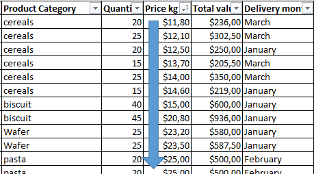
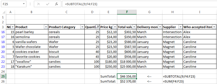
We need to extract from the database products that were purchased in lots of 25 kg or more. For this purpose click the filter arrow on QUANTITY cell, and select the following options.
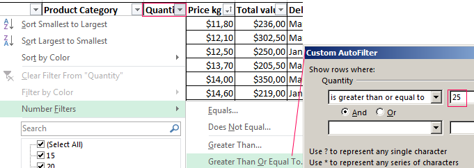
In the window that appears in front of condition БОЛЬШЕ ИЛИ РАВНО inscribe number 25. Then you will get sample indicating the products ordered by the lots greater than 25 kg or equal to this. Those products also sorted in the manner of its price growth since we did not remove sorting by price.
Subtotals
This is another useful function which allows calculating the sum, the multiplication, minimum or average value, etc. using the existing database. It is called the subtotals. =SUBTOTAL() This function has one main advantage. It allows making calculations with certain function even if you change the size of the table. Let’s consider it with an example.
Let us give our full database suitable view. Next we create a formula for the AutoSum in column Total value. Enter formula writing it in the F26 cell. At the same time remember how database sorting in Excel: number of rows fixed in place. Therefore the formula will still be in the F26 cell even when we do filtering.
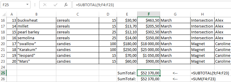
Subtotal function has 30 arguments. The first is static: the action code. By default Excel set code number 9, so let it be. The second and subsequent arguments are dynamic: this is links to ranges which are summed up. We have a range: F4: F24. It turned out 19,670 rubles.
Now try again to sort number, leaving only a party of 25 kg and >.
We see that the amount has changed, too.
In Excel, you can also create a small database and easy to work with them. When large volumes of data is very convenient and efficient.
Источник
Excel database functions fix some, but not all, of the problems with long SUMIFS and SUMPRODUCT formulas.
For example, formulas that use SUMIFS and SUMPRODUCT are often difficult to enter and understand, sometimes dates don’t work correctly, and it’s difficult to set up criteria such as orders that match a certain date range AND a certain Sales Rep but NOT a certain industry.
Database Functions Definition: Excel database functions allow you to sum and count data in spreadsheets based on AND and OR conditions that join together multiple sets of criteria, such as dates, amounts, geographies, industries, and product identifiers.
Database functions do require more time to set up because you must create extra rows in the spreadsheet, and you must get the syntax exactly right, or nothing will work.
A basic Database function setup might look like this:

Some of the key Excel database functions include the following:
=DSUM: Add numbers in a field (i.e., table column) that match specific conditions
=DCOUNT: Count # cells in a field (i.e., a table column) that match specific conditions
=DCOUNTA: Same, but only for nonblank cells
=DGET: Extracts single row from table that matches specific conditions
How Database Functions Work
A few notes on the functionality in the screenshot above:
1) The order of the fields in this area must be the same as the order of the fields in the table itself (Order_Table). If Order Date follows Amount in the table, Order Date must follow Amount here:

2) You do NOT need to use all the fields in the table – you can choose any of them. We only use a few fields from the table here.
3) And you can repeat the same field multiple times as long as the repeats are all entered after the first entry, with nothing in between.
4) In a single row, the conditions are joined with AND. In other words, for the first row here, matching entries must be in the “Industrials” industry, the “Midwest” region, AND between January 1, 2021 and December 31, 2024.
5) Multiple rows are joined with OR. So, in the example above, matching entries must be in the “Industrials” industry, the “Midwest” region, AND between January 1, 2021 and December 31, 2024… OR they must be in the “Energy” industry, the “Northeast” region, AND between January 1, 2021 and December 31, 2024.
6) The last part – Summary!$J$6:$P$8 – cannot include empty rows, or Database functions such as DSUM will sum up the entire table.
Database functions are most useful for writing queries with complex criteria, such as ones that involve multiple dates, amounts, regions, industries, and more.
They tend to be overkill for simple queries, such as summing up all orders between two dates, or summing up all orders in a certain industry; for those, SUMIFS and SUMPRODUCT are fine.
The Most Common Functions
The most common Database function is DSUM, which looks at all the rows in a table and sums up a specific field (column) in each matching row:
=DSUM(Database, Field, Criteria)
The Database part is the range of cell references, which must contain the field names in the header. This range should ideally be a Data Table, but it can be any range of cells in the spreadsheet.
The Field part is the column or field you want to add up or count. You can use a column number or the exact name in text; it’s best to create a direct link to the title in the table header to avoid errors.
The Criteria part is the smaller range we created above: Summary!$J$6:$P$8.
It must include at least one field name that’s in the Database AND at least one other condition to be evaluated. If it does not, DSUM will sum up everything in the table.
Each function mentioned above – DSUM, DCOUNT, DCOUNTA, and DGET – accepts these same inputs: Database, Field, and Criteria.
All the normal operators, such as <, >, <=, >=, <>, =, *, and ?, still work in the Criteria range of cells, but only if they make logical sense for the underlying data.
The biggest problem with Database functions is that it’s extremely easy to make a small mistake that results in the entire function not working.
For example:

Why did these functions suddenly stop working? Because we hard-coded the “Region” field in the header and added an extra space at the end:

This problem shows you why it’s best to link directly to the field names in the Order Table here.
Besides this issue, another drawback of database functions is that it’s not easy to see trends and patterns when you use them.
For example, how have sales to Energy companies changed over 5-10 years? What percentage of total sales did they represent each year, and which sales reps were most responsible?
For those types of tasks, you are better off using pivot tables and related functionality, such as Power Pivot, which we cover in our Excel & Fundamentals course.
Excel Database Functions Multiple Criteria
If you want to set up a function with multiple criteria, remember the rules above: individual fields in a row are joined together with an AND, and individual rows are joined together with an OR.
Therefore, the following function:

Will do the following:
1) First, it will find and add all Order Amounts in the Industrials industry AND in the Midwest AND placed between January 1, 2021 and December 31, 2024 (inclusive).
2) Then, it will find and add all Order Amounts in the Industrials industry AND in the Northeast AND placed between January 1, 2021 and December 31, 2024 (inclusive).
3) Next, it will find and add all Order Amounts in the Energy industry AND in the Midwest AND placed between January 1, 2021 and December 31, 2024 (inclusive).
4) Finally, it will find and add all Order Amounts in the Energy industry AND in the Northeast AND placed between January 1, 2021 and December 31, 2024 (inclusive).
Since each row is joined with an OR, the function will then add up all these Order Amounts.
When you enter multiple rows of criteria, you always get results that match any of the rows.
Database functions have their uses, but we tend to use them less than sensitivity analysis in financial models and less than pivot tables in data analysis.
Combined shape 37
Created with Sketch.
Based on the content of this tutorial, our recommended Premium Course Upgrade is…
Other BIWS Courses Include:
Polygon 1
Created with Sketch.
BIWS Premium:
Get the Excel & VBA, Financial Modeling Mastery, and PowerPoint Pro courses together and learn everything from Excel shortcuts up through advanced modeling, VBA to automate your workflow, and PowerPoint and presentation skills.
Learn More
Polygon 1
Created with Sketch.
BIWS Platinum:
The most comprehensive package on the market today for investment banking, private equity, hedge funds, and other finance roles. Includes ALL the courses on the site, plus updates and any new courses in the future.
Learn More