
Microsoft Word allows you count text, but what about Excel? If you need a count of your text in Excel, you can get this by using the COUNTIF function and then a combination of other functions depending on your desired result.
How to count text in Excel
If you want to learn how to count text in Excel, you need to use function COUNTIF with the criteria defined using wildcard *, with the formula: =COUNTIF(range;"*"). Range is defined cell range where you want to count the text in Excel and wildcard * is criteria for all text occurrences in the defined range.
Some interesting and very useful examples will be covered in this tutorial with the main focus on the COUNTIF function and different usages of this function in text counting. Limitations of COUNTIF function have been covered in this tutorial with an additional explanation of other functions such as SUMPRODUCT/ISNUMBER/FIND functions combination. After this tutorial, you will be able to count text cells in excel, count specific text cells, case sensitive text cells and text cells with multiple criteria defined – which is a very good base for further creative Excel problem-solving.
Count Text Cells in Excel
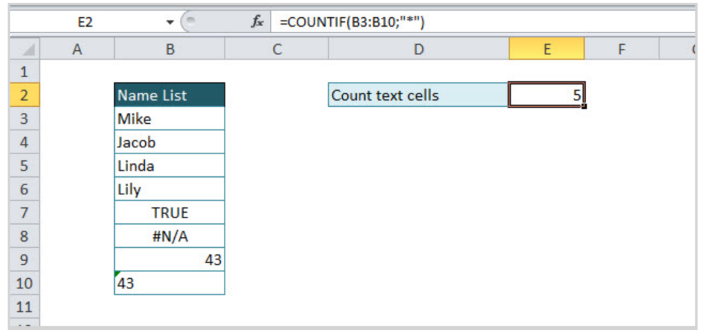
Text Cells can be easily found in Excel using COUNTIF or COUNTIFS functions. The COUNTIF function searches text cells based on specific criteria and in the defined range. As in the example below, the defined range is table Name list, and text criteria is defined using wildcard “*”. The formula result is 5, all text cells have been counted. Note that number formatted as text in cell B10 is also counted, but Booleans (TRUE /FALSE) and error (#N/A) are not recognized as text.
The formula for counting text cells:
=COUNTIF(range;"*")
For counting non-text cells, the formula should be a little bit changed in criteria part:
=COUNTIF(range;"<>*")
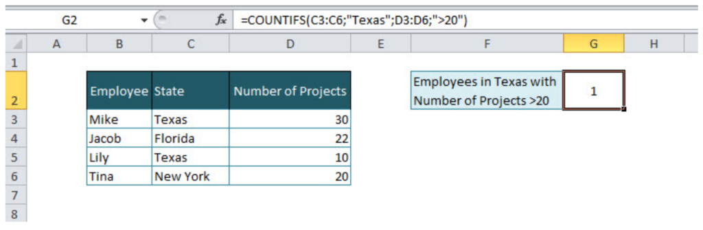
If there are several criteria for counting cells, then COUNTIFS function should be used. For example, if we want to count the number of employees from Texas with project number greater than 20, then the function will look like:
=COUNTIFS(C3:C6;"Texas";D3:D6;">20").
In criteria range in column State, a specific text criteria is defined under quotations “Texas”. The second criteria is numeric, criteria range is column Number of projects, and criteria is numeric value greater than 20, also under quotations “>20”. If we were looking for exact value, the formula would look like:
=COUNTIFS(C3:C6;"Texas";D3:D6;20)
Count Specific Text in Cells
For counting specific text under cells range, COUNTIF function is suitable with the formula:
=COUNTIF(range;"*text*")
=COUNTIF(B3:B9;"*Mike*")
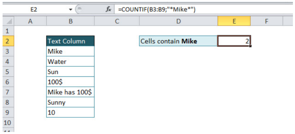
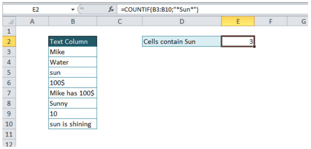
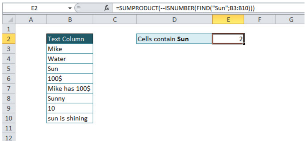
The first part of the formula is range and second is text criteria, in our example “*Mike*”. If wildcard * has not been used before and after criteria text, formula result would have been 1 (Formula would find cells only with word Mike). Wildcard * before and after criteria text, means that all cells that contain criteria characters will be taken into account. As in another example below with text criteria Sun, three cells were found (sun, Sunny, sun is shining)
=COUNTIF(B3:B10;"*Sun*")
Note: The COUNTIF function is not case sensitive, an alternative function for case sensitive text searches is SUMPRODUCT/FIND function combination.
Count Case Sensitive Specific Text
For a case-sensitive text count, a combination of three formulas should be used: SUMPRODUCT, ISNUMBER and FIND. Let’s look in the example below. If we want to count cells that contain text Sun, case sensitive, COUNTIF function would not be the appropriate solution, instead of this function combination of three functions mentioned above has to be used.
=SUMPRODUCT(--ISNUMBER(FIND("Sun";B3:B10)))
We should go through a separate function explanation in order to understand functions combination. FIND function, searches specific text in the defined cell, and returns the number of the starting position of the text used as criteria. This explanation is relevant, if the searching range is just one cell. If we want to use FIND function in a range of the cells, then the combination with SUMPRODUCT function is necessary.
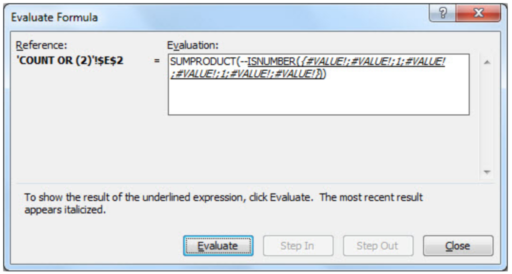
Without ISNUMBER, function combination of FIND and SUMPRODUCT functions would return an error. ISNUMBER function is necessary because whenever FIND function does not match defined criteria, the output will be an error, as in print screen below of the evaluated formula.
In order to change error values with Boolean TRUE/FALSE statement, ISNUMERIC formula should be used (defining numeric values as TRUE, and non-numeric as FALSE, as in print screen below).
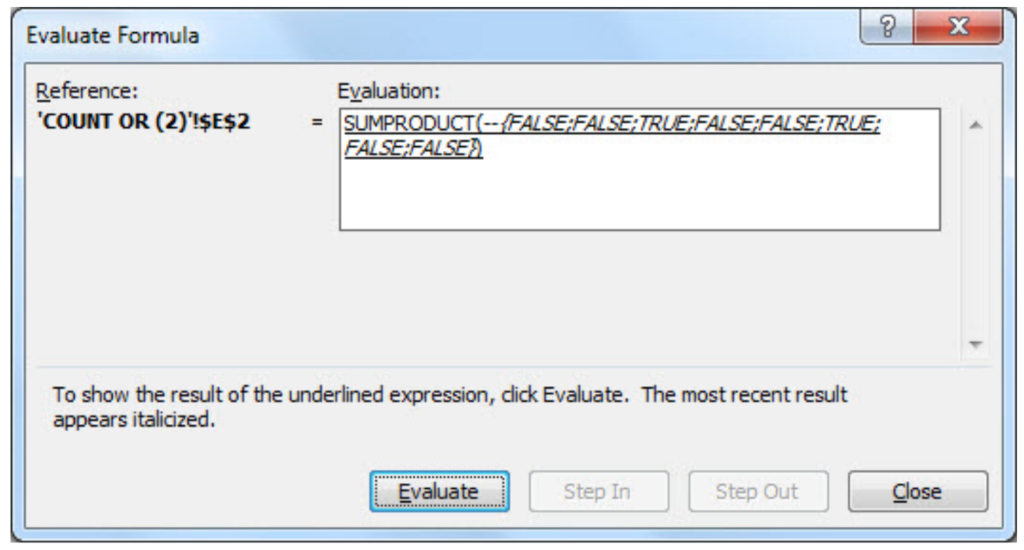
You might be wondering what character — in SUMPRODUCT function stands for. It converts Boolean values TRUE/FALSE in numeric values 1/0, enabling SUMPRODUCT function to deal with numeric operations (without character — in SUMPRODUCT function, the final result would be 0).
Remember, if you want to count specific text cells that are not case sensitive, COUNTIF function is suitable. For all case sensitive searches combination of SUMPRODUCT/ISNUMBER/FIND functions is appropriate.
Count Text Cells with Multiple Criteria
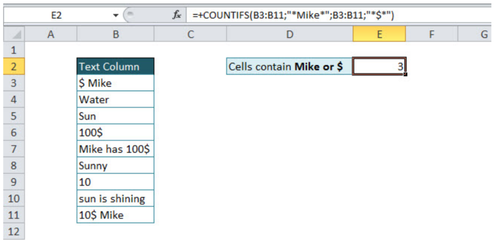
If you want to count cells with Multiple criteria, with all criteria acceptable, there is an interesting way of solving that problem, a combination of SUMPRODUCT/ISNUMBER/FIND functions. Please take a look in the example below. We should count all cells that contain either Mike or $. Tricky part could be the cells that contain both Mike and $.
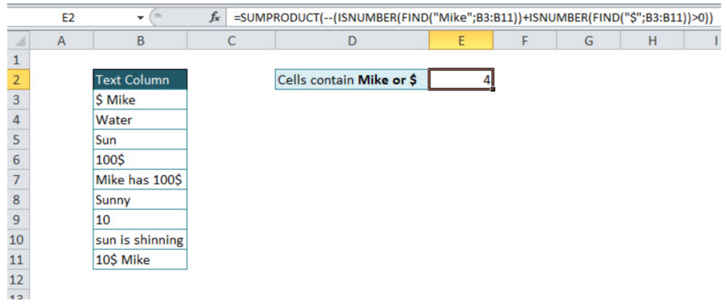
=SUMPRODUCT(--(ISNUMBER(FIND("Mike";B3:B11))+ISNUMBER(FIND("$";B3:B11))>0))
Formula just looks complex, in order to be easier for understanding, I will divide it into several steps. Also, knowledge from the previous tutorial point will be necessary for further work, since the combination of FIND, ISNUMBER, and SUMPRODUCT functions have been explained.
In the first part of the function, we loop through the table and find cells that contain Mike:
=ISNUMBER(FIND("Mike";B3:B11))
The output of this part of the function will be an array with values {1;0;0;0;1;0;0;0;1}, number 1, where criteria have been met, and 0, where has not.
In the second part of the function, looping criteria is $, counting cells containing this value:
=ISNUMBER(FIND("$";B3:B11))
The output of this part of the function will be an array with values {1;0;0;1;1;0;0;0;1}, number 1, where criteria have been met, and 0, where has not.
Next step is to sum these two arrays, since cell should be counted if any of conditions is fulfilled:
=ISNUMBER(FIND("Mike";B3:B11))+ISNUMBER(FIND("$";B3:B11))
The output of this step is {2;0;0;1;2;0;0;0;2}, the number greater than 0 means that one of the condition has been met (2 – both conditions, 1 – one condition)
Without function part >0, the final function would double count cells that met both conditions and the final result would be 7 (sum of all array numbers). In order to avoid it, in the formula should be added >0:
=ISNUMBER(FIND("Mike";B3:B11))+ISNUMBER(FIND("$";B3:B11))>0
The output of this step is array {1;0;0;1;1;0;0;0;1}, the previous array has been checked and only values greater than 0 are TRUE (in an array have value 1), and others are FALSE (in an array have value 0).
Final output of the formula is the sum of the final array values, 4.
Looks very confusing, but after several usages, you will become familiar with this functions.
At the end, we will cover one more multiple criteria text count function, already mentioned in the tutorial, COUNTIFS function. In order to distinguish the usage of functions mentioned above and COUNTIFS function, two words are enough OR/AND. If you want to count text cells with multiple criteria but all conditions have to be met at the same time, then COUNTIFS function is appropriate. If at least one condition should be met, then the combination of function explained above is suitable.
Look at the example below, the number of cells that contain both Mike and $ is easily calculated with COUNTIFS function:
=COUNTIFS(range1;"*text1*";range2;"*text2*")
=COUNTIFS(B3:B11;"*Mike*";B3:B11;"*$*")
In the defined range, function counts only cells where both conditions have been met. The final result is 3.
Still need some help with Excel formatting or have other questions about Excel? Connect with a live Excel expert here for some 1 on 1 help. Your first session is always free.
In this example, the goal is to count cells in a range that contain text values. This could be hardcoded text like «apple» or «red», numbers entered as text, or formulas that return text values. Empty cells, and cells that contain numeric values or errors should not be included in the count. This problem can be solved with the COUNTIF function or the SUMPRODUCT function. Both approaches are explained below. For convenience, data is the named range B5:B15.
COUNTIF function
The simplest way to solve this problem is with the COUNTIF function and the asterisk (*) wildcard. The asterisk (*) matches zero or more characters of any kind. For example, to count cells in a range that begin with «a», you can use COUNTIF like this:
=COUNTIF(range,"a*") // begins with "a"
In this example however we don’t want to match any specific text value. We want to match all text values. To do this, we provide the asterisk (*) by itself for criteria. The formula in H5 is:
=COUNTIF(data,"*") // any text value
The result is 4, because there are four cells in data (B5:B15) that contain text values.
To reverse the operation of the formula and count all cells that do not contain text, add the not equal to (<>) logical operator like this:
=COUNTIF(data,"<>*") // non-text values
This is the formula used in cell H6. The result is 7, since there are seven cells in data (B5:B15) that do not contain text values.
COUNTIFS function
To apply more specific criteria, you can switch to the COUNTIFs function, which supports multiple conditions. For example, to count cells with text, but exclude cells that contain only a space character, you can use a formula like this:
=COUNTIFS(range,"*",range,"<> ")
This formula will count cells that contain any text value except a single space (» «).
SUMPRODUCT function
Another way to solve this problem is to use the SUMPRODUCT function with the ISTEXT function. SUMPRODUCT makes it easy to perform a logical test on a range, then count the results. The test is performed with the ISTEXT function. True to its name, the ISTEXT function only returns TRUE when given a text value:
=ISTEXT("apple")// returns TRUE
=ISTEXT(70) // returns FALSE
To count cells with text values in the example shown, you can use a formula like this:
=SUMPRODUCT(--ISTEXT(data))
Working from the inside out, the logical test is based on the ISTEXT function:
ISTEXT(data)
Because data (B5:B15) contains 11 values, ISTEXT returns 11 results in an array like this:
{TRUE;TRUE;TRUE;FALSE;FALSE;TRUE;FALSE;FALSE;FALSE;FALSE;FALSE}
In this array, the TRUE values correspond to cells that contain text values, and the FALSE values represent cells that do not contain text. To convert the TRUE and FALSE values to 1s and 0s, we use a double negative (—):
--{TRUE;TRUE;TRUE;FALSE;FALSE;TRUE;FALSE;FALSE;FALSE;FALSE;FALSE}
The resulting array inside the SUMPRODUCT function looks like this:
=SUMPRODUCT({1;1;1;0;0;1;0;0;0;0;0}) // returns 4
With a single array to process, SUMPRODUCT sums the array and returns 4 as the result.
To reverse the formula and count all cells that do not contain text, you can nest the ISTEXT function inside the NOT function like this:
=SUMPRODUCT(--NOT(ISTEXT(data)))
The NOT function reverses the results from ISTEXT. The double negative (—) converts the array to numbers, and the array inside SUMPRODUCT looks like this:
=SUMPRODUCT({0;0;0;1;1;0;1;1;1;1;1}) // returns 7
The result is 7, since there are seven cells in data (B5:B15) that do not contain text values.
Note: the SUMPRODUCT formulas above may seem complex, but using Boolean operations in array formulas is powerful and flexible. It is also an important skill in modern functions like FILTER and XLOOKUP, which often use this technique to select the right data. The syntax used by COUNTIF on the other hand is unique to a group of eight functions and is therefore not as useful or portable.
Home > Microsoft Excel > How to Count Cells with Text in Excel? 3 Different Use Cases
(Note: This guide on how to count cells with text in Excel is suitable for all Excel versions including Office 365)
Excel deals with a variety of data of diverse data types. Excel can accept data in the form of numbers, text, characters, and operators. When storing large amounts of data, sorting and retrieving one particular type of data can be quite difficult.
In a spreadsheet consisting of different data types, you might sometimes have to pinpoint the cells with text and count them to perform any function or operation.
In this article, I will tell you how to count cells with text in Excel along with their use cases.
You’ll Learn:
- What Is Count in Excel?
- How to Count Cells with Text in Excel?
- Count All the Text Values
- Count Cells with Text Value Without Blank Spaces
- Count Cells with a Particular Text Value
- Reminders
Watch our video on how to count cells with text in Excel

Related Reads:
How to Count Unique Values in Excel? 3 Easy Ways to Count Unique and Distinct Values
How to Apply the Accounting Number Format in Excel? (3 Best methods)
How to Use Excel COUNTIFS: The Best Guide
What Is Count in Excel?
Before we learn how to count cells with text in Excel, let us refresh the concept of COUNT in Excel. Let us see what COUNT is and how Excel counts the values.
Counting is one of the most commonly used functions in Excel which provides a numerical summary of the total values which might be useful in a variety of places. In simpler terms, Excel counts how many times a value appears in a column or row.
In Excel, you can count the number of cells or the values it houses by using functions. Excel has a variety of functions that help in counting. Functions like COUNT and COUNTA are used to count all the cells in a particular range or select cells which house a particular value. On the other hand, COUNTIF and COUNTIFS functions count cells only if they satisfy a particular value.
In the case where we want to count the number of cells with text in Excel, the function COUNTIF/COUNTIFS is the best choice. Using these functions, you can set criteria to the function so it counts only the cells which house the text values in the cell.
How to Count Cells with Text in Excel?
Texts are also called strings in Excel. When it comes to technological terms, strings are a block of text which might contain any identifying values. They can be individual values like name or address, or they can be a variable that points to another constant.
In Excel, they are usually written with alphanumeric characters which are enclosed by double quotation marks or can be written with an apostrophe. Additionally, they can be a result of logical functions like TRUE or FALSE, or may even be special characters like !, @, #, and $.
Count All the Text Values
To count all the text values in the given Excel sheet, you can use the COUNTIF function along with a wildcard character. This function with a wildcard counts all the text values in a given range.
To count the cells with text in Excel, choose a destination cell and enter the formula =COUNTIF(range,criteria). Here, the range denotes the array of cells within which you want the function to act. The criteria variable denotes the condition to satisfy when counting the values.
Consider the below given example. To find the cells with text values in a given range, enter the formula =COUNTIF(A3:A10,”*”). The function COUNTIF acts on the cell range A3 to A10 and finds the text values. The * represents the wildcard element. The * symbol specifies anything other than numbers to be counted, including blank spaces and special characters. However, this method does not count logical values.

The cells with text within a given range are found to be 7. If you count the values manually, you will notice that the cells with text values are 5. But, the cells A11 and A12 also contain characters like space ( ) and apostrophe (‘) which do not show up in the cell.
Also Read:
How to Hide Formulas in Excel? 2 Different Approaches
How to Select Non Adjacent Cells in Excel? 5 Simple Ways
How to Rotate Text in Excel? 3 Effective Ways
Count Cells with Text Value Without Blank Spaces
You can use the same COUNTIF function and wildcards to count the number of cells with text in them. This method only counts cells that hold any text value and does not count any blank cell in the given range.
To count the cells which have text value in them, enter the formula =COUNTIF(range,criteria) in the destination cell. This is the same as the previous case, but adding wildcard “?” together with “*” only counts the cells which have text values.
Consider the below given example. To find the cells with text values in a given range, enter the formula =COUNTIF(A3:A12,”?*”). Here, the function COUNTIF counts the number of cells in the range of cells A3 to A12. Whereas for the criteria parameter, instead of just passing “*” which counts all the cells with text values, adding the “?” wildcard to the criteria counts the cells which have at least one character.

As result, the cells which have text values are found to be 6. You can see the text values aligned to the left of the cell whereas the numerical values are aligned to the right of the cell. This function also counts the apostrophe as a text character, but it does not count the blank spaces.
Count Cells with a Particular Text Value
With the help of wildcards and the COUNTIF function, you can also count the cells with any specific text values in Excel.
Using this method, you’ll learn how to count specific words in Excel. To count the cells with the specific value, you can just enter the text to count within quotations when you pass the criteria parameter.
Let me show you an example. Suppose you want to count the occurrences of the word “two” in a range of cells. You can just enter the formula in the =COUNTIF(A3:A12,”two”) to count the occurrences of the word “two” in the given range of cells A3 to A12.

Wildcards can be used to count cells with a specific text value.
Imagine you want to count the number of cells that contain the text starting with any particular letter or character. Say, you want to count the number of cells that starts with the letter “t”, then you can use the “*” wildcard.
Consider the example, in the cell range A3 to A12 you want to count the number of cells which start with the letter “t”. Then, enter the function =COUNTIF(A3:A12,“t*”) in the destination cell.

The resultant value is 2. This denotes that when you want to find the cells which start with the letter “t”, you can enter the value “t*” in the criteria parameter. As a result, the COUNTIF function counts the cells which start with the letter “t” irrespective of the number of characters that follow them.
Another case to use the wildcard is to count any one particular value. For example, if you want to find the occurrences of a three-letter word that have the starting letter “t” and ends with “o”, you can use the “?” wildcard. As the “*” wildcard replaces any number of characters, the “?” wildcard only replaces one character.

In this case, the count function only counts the cells with three characters which start with “t” and end with “o” and counts them.
Suggested Reads:
How to Use SUMPRODUCT Function in Excel? 5 Easy Examples
How to Use the PROPER Function in Excel? 3 Easy Examples
Excel DATEVALUE – A Step-by-Step Guide
Reminders
- Wildcards can take the place of characters and are of three types: *, ?, and ~. Use the * wildcard when you want to replace more than one character, use the ? wildcard to replace exactly one character, and ~ to replace and search for the exact character. Wildcards are not case-sensitive. Additionally, wildcards only work on text and not on numbers.
- Sometimes when a cell appears blank, it does not necessarily mean that the cell is empty. Characters like space ( ), apostrophe (‘), and double quotation marks(””) also make the cell look empty. But technically, they are considered text.
- When looking for cells with text manually, you can easily distinguish the text from the number in Excel. Numbers are aligned to the right of the cell, whereas text is aligned to the left of the cell.
Frequently Asked Questions
How do I count all the cells in Excel?
To count all the cells within a particular range in Excel, you can use the COUNT function followed by the range of cells that you want to count i.e =COUNT(range).
How to count the number of blank cells in Excel?
You can use the COUNTIF or COUNTIFS function with an empty string (““) as the criteria parameter i.e =COUNTIF(range,””) to count the number of blank/empty cells. Or, you can use the =COUNTBLANK(range) function to count them.
How to count in a PivotTable?
In a PivotTable, you can automatically set a category and add fields in the Value Field Setting to count the values.
Closing Thoughts
In this article, we saw how to count cells with text in Excel. Additionally, we saw all the ways you can use the COUNTIF function to count the text values without including the blank spaces and counting cells with particular words.
If you need more high-quality Excel guides, please check out our free Excel resources center. Simon Sez IT has been teaching Excel for over ten years. For a low, monthly fee you can get access to 130+ IT training courses. Click here for advanced Excel courses with in-depth training modules.
Simon Calder

Chris “Simon” Calder was working as a Project Manager in IT for one of Los Angeles’ most prestigious cultural institutions, LACMA.He taught himself to use Microsoft Project from a giant textbook and hated every moment of it. Online learning was in its infancy then, but he spotted an opportunity and made an online MS Project course — the rest, as they say, is history!
На чтение 6 мин. Просмотров 17.5k.
Есть одна штука, которую я бы хотел иметь в Excel: подсчет слов в ячейке.
Если вы работаете в MS Word, в строке состояния есть встроенная опция, которая показывает, сколько слов на листе.
В Word есть опция для подсчета слов, но не в Excel. Вы можете посчитать количество ячеек, в которых есть текст, но не фактические слова в них.
В Excel в нашем распоряжении есть функции, с которыми мы можем посчитать почти все. Вы можете создать формулу, которая сможет посчитать слова в ячейке.
Содержание
- Четыре разных способа посчитать слова в Excel
- 1. Формула для подсчета слов в ячейке
- 2. Подсчет слов в диапазоне ячеек
- 3. Подсчет количества слов во всей таблицы с кодом VBA
- 4. Подсчет определенного слова/текстовой строки в диапазоне
- Заключение
Четыре разных способа посчитать слова в Excel
Сегодня в этой статье вы научитесь считать слова в Excel в ячейке или диапазоне ячеек или даже во всей таблице.
Также я покажу вам, как посчитать определенное слово из диапазона ячеек. Теперь без всяких церемоний, давайте начнем.
1. Формула для подсчета слов в ячейке
Сочетание функций ДЛСТР с ПОДСТАВИТЬ
И формула будет (текст в ячейке A1):
= ДЛСТР(A1) — ДЛСТР (ПОДСТАВИТЬ (A1; » «; «»)) + 1
Когда вы ссылаетесь на ячейку, используя эту формулу, она вернет 5 в результате.

И да, у вас есть 5 слов в ячейке.
Как формула работает?
Прежде чем перейти к этой формуле, просто подумайте. В обычном предложении, если у вас восемь слов, у вас определенно будет 7 пробелов в этих словах. Правильно? Это означает, что у вас всегда будет на одно слово больше, чем пробелов.
Идея проста: если вы хотите посчитать слова, подсчитайте пробелы и добавьте единицу.
Теперь, чтобы понять эту формулу, вам нужно разделить ее на три части.

В первой части мы использовали функцию ДЛСТР (LEN) для подсчета количества символов в ячейке A1. А во второй и третьей части мы объединили ПОДСТАВИТЬ (SUBSTITUTE) с ДЛСТР (LEN), чтобы удалить пробелы из ячейки и затем подсчитать символы.
Наше уравнение выглядит так:
= 20 — 16 +1
- 20 — общее количество символов с пробелами
- 16 — символы без пробелов
Когда вы вычтете одно из другого, вы получите количество пробелов, и вам останется добавить один. В результате возвращается число 5, что является общим количеством слов в ячейке.
Когда вы используете приведенную выше формулу, она вернет 1, даже если ячейка пуста, поэтому лучше обернуть ее функцией ЕСЛИ (IF), чтобы избежать этой проблемы.
= ЕСЛИ(ЕПУСТО (A1);0; ДЛСТР(A1) — ДЛСТР(ПОДСТАВИТЬ(A1; » «; «»)) + 1)
Эта формула сначала проверяет ячейку и возвращает количество слов, только если в ячейке есть значение.

Пользовательская функция
Помимо приведенных выше формул, я напишу вам небольшой код для создания Пользовательской функции. Этот код поможет вам создать пользовательскую функцию, которая будет просто возвращать количество слов. Короче говоря, вам не нужно будет сочетать какие-либо функции.
Function MyWordCount(rng As Range) As Integer

MyWordCount = UBound(Split(rng.Value, " "), 1) + 1

End Function
Давайте я расскажу вам, как ее использовать.
- Прежде всего, введите этот код в редакторе VBA.

- Затем вернитесь на свой рабочий лист и введите «= MyWordCount(» и сошлитесь на ячейку, в которой у вас есть значение.
И она вернет количество слов.

2. Подсчет слов в диапазоне ячеек
Теперь давайте перейдем на следующий уровень. Здесь вам нужно будет посчитать слова уже в диапазоне ячеек вместо одной ячейки.
Хорошая новость! Можно использовать ту же формулу (добавив небольшое изменение), которую мы использовали выше.
Вот эта формула:
= СУММПРОИЗВ(ДЛСТР(A1:A11)-ДЛСТР(ПОДСТАВИТЬ(A1:A11; » «;»»))+1)

В приведенной выше формуле A1: A11 — это диапазон ячеек, при вводе формулы в результате получим 55.
Как это работает?
Эта формула работает так же, как и первый метод, но только чуть сложнее. Разница лишь в том, что мы завернули ее в СУММПРОИЗВ (SUMPRODUCT) и ссылаемся на весь диапазон вместо одной ячейки.

Вы помните, что СУММПРОИЗВ (SUMPRODUCT) может работать с массивами? Поэтому, когда вы используете эту функцию, она возвращает массив, в котором у вас есть количество слов для каждой ячейки. Далее она суммирует эти цифры и сообщает вам количество слов в столбце.
3. Подсчет количества слов во всей таблицы с кодом VBA
Этот код является одним из списка полезных макросов, который я использую в своей работе, и он может помочь вам подсчитать все слова на листе.
Sub Word_Count_Worksheet()

Dim WordCnt As Long

Dim rng As Range

Dim S As String

Dim N As Long

For Each rng In ActiveSheet.UsedRange.Cells

S = Application.WorksheetFunction.Trim(rng.Text)

N = 0

If S <> vbNullString Then

N = Len(S) - Len(Replace(S, " ", "")) + 1

End If

WordCnt = WordCnt + N

Next rng

MsgBox "Всего " & Format(WordCnt, "#,##0") & " слов на активном листе"

End Sub
Когда вы запустите его, он покажет окно сообщения с количеством слов, которые у вас есть в активном листе.

4. Подсчет определенного слова/текстовой строки в диапазоне
Здесь у нас другая ситуация. Допустим, нам нужно посчитать определенное слово в диапазоне ячеек или проверить, сколько раз значение появляется в столбце.
Разберем на примере.
Ниже у нас есть диапазон из четырех ячеек, и из этого диапазона нам нужно посчитать количество появлений слова «понедельник».
Вот формула для этого:
= СУММПРОИЗВ ((ДЛСТР (A1:A4) — ДЛСТР (ПОДСТАВИТЬ (A1:A4; «понедельник»; «»)) / ДЛСТР(«понедельник»))

И когда вы введете ее, она возвратит количество понедельников. Ответ — 4.
Формула возвращает количество слов (частоту слова) в диапазоне, а не количество ячеек, в которых есть это слово.
Понедельник встречается четыре раза в трех ячейках.
Как это работает?
Чтобы понять эту функцию, вам снова нужно разделить ее на четыре части.
В первой части функция ДЛСТР (LEN) возвращает массив количества символов в ячейках.

Вторая часть возвращает массив подсчета символов в ячейках, удалив слово «понедельник».

В третьей части функция ДЛСТР (LEN) возвращает длину символов слова «понедельник».

После этого вычитаем первую часть из второй, а затем делим ее на третью часть. Возвращен массив с количеством слов «понедельник» в каждой ячейке.

В четвертой части СУММПРОИЗВ (SUMPRODUCT) возвращает сумму этого массива и дает количество понедельников в диапазоне.
Заключение
Всякий раз, когда вы печатаете какой-то текст в ячейке или диапазоне ячеек, вы можете использовать эти методы для контроля количества слов.
Я мечтаю, что когда-нибудь в будущем в Excel появится эта опция. Ну а пока будем пользоваться этими замечательными методами.
Я надеюсь, что статья была полезной для вас. Какой метод вам понравился больше всех?
Не забудьте поделиться своими мнениями со мной в разделе комментариев, для меня это важно. И, пожалуйста, не забудьте поделиться со своими друзьями, я уверен, что они это оценят.
Содержание
- Count characters in cells
- Give it a try
- Description of formulas to count the occurrences of text, characters, and words in Excel
- Summary
- More Information
- Formula to Count the Number of Occurrences of a Text String in a Range
- Example 1: Counting the Number of Occurrences of a Text String in a Range
- Formula to Count the Number of Occurrences of a Single Character in One Cell
- Example 2: Counting the Number of Occurrences of a Character in One Cell
- Formula to Count the Number of Occurrences of a Single Character in a Range
- Example 3: Counting the Number of Occurrences of a Character in a Range
- Formula to Count the Number of Words Separated by a Character in a Cell
- Example 4: Counting the Number of Words Separated by a Space in a Cell
- References
- Ways to count values in a worksheet
- Download our examples
- In this article
- Simple counting
- Video: Count cells by using the Excel status bar
- Use AutoSum
- Add a Subtotal row
- Count cells in a list or Excel table column by using the SUBTOTAL function
- Counting based on one or more conditions
- Video: Use the COUNT, COUNTIF, and COUNTA functions
- Count cells in a range by using the COUNT function
- Count cells in a range based on a single condition by using the COUNTIF function
- Count cells in a column based on single or multiple conditions by using the DCOUNT function
- Count cells in a range based on multiple conditions by using the COUNTIFS function
- Count based on criteria by using the COUNT and IF functions together
- Count how often multiple text or number values occur by using the SUM and IF functions together
- Count cells in a column or row in a PivotTable
- Counting when your data contains blank values
- Count nonblank cells in a range by using the COUNTA function
- Count nonblank cells in a list with specific conditions by using the DCOUNTA function
- Count blank cells in a contiguous range by using the COUNTBLANK function
- Count blank cells in a non-contiguous range by using a combination of SUM and IF functions
- Counting unique occurrences of values
- Count the number of unique values in a list column by using Advanced Filter
- Count the number of unique values in a range that meet one or more conditions by using IF, SUM, FREQUENCY, MATCH, and LEN functions
- Special cases (count all cells, count words)
- Count the total number of cells in a range by using ROWS and COLUMNS functions
- Count words in a range by using a combination of SUM, IF, LEN, TRIM, and SUBSTITUTE functions
- Displaying calculations and counts on the status bar
- Need more help?
Count characters in cells
When you need to count the characters in cells, use the LEN function—which counts letters, numbers, characters, and all spaces. For example, the length of «It’s 98 degrees today, so I’ll go swimming» (excluding the quotes) is 42 characters—31 letters, 2 numbers, 8 spaces, a comma, and 2 apostrophes.
To use the function, enter =LEN( cell ) in the formula bar, then press Enter on your keyboard.
Multiple cells: To apply the same formula to multiple cells, enter the formula in the first cell and then drag the fill handle down (or across) the range of cells.
To get the a total count of all the characters in several cells is to use the SUM functions along with LEN. In this example, the LEN function counts the characters in each cell and the SUM function adds the counts:
Give it a try
Here are some examples that demonstrate how to use the LEN function.
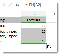
Copy the table below and paste it into cell A1 in an Excel worksheet. Drag the formula from B2 to B4 to see the length of the text in all the cells in column A.
The quick brown fox.
The quick brown fox jumped.
The quick brown fox jumped over the lazy dog.
Count characters in one cell
The formula counts the characters in cell A2, which totals to 27—which includes all spaces and the period at the end of the sentence.
NOTE: LEN counts any spaces after the last character.
Count characters in multiple cells
Press Ctrl+C to copy cell B2, then select cells B3 and B4, and then press Ctrl+V to paste its formula into cells B3:B4.
This copies the formula to cells B3 and B4, and the function counts the characters in each cell (20, 27, and 45).
Count a total number of characters
In the sample workbook, click cell B6.
In the cell, enter =SUM(LEN(A2),LEN(A3),LEN(A4)) and press Enter.
This counts the characters in each of the three cells and totals them (92).
Источник
Description of formulas to count the occurrences of text, characters, and words in Excel
Summary
This article contains and describes formulas that calculate the following:
- The number of occurrences of a text string in a range of cells.
- The number of occurrences of a character in one cell.
- The number of occurrences of a character in a range of cells.
- The number of words (or text strings) separated by a character in a cell.
More Information
Formula to Count the Number of Occurrences of a Text String in a Range
=SUM(LEN(range)-LEN(SUBSTITUTE(range,»text»,»»)))/LEN(«text»)
Where range is the cell range in question and «text» is replaced by the specific text string that you want to count.
The above formula must be entered as an array formula. To enter a formula as an array in Excel for Windows, press CTRL+SHIFT+ENTER. To enter a formula as an array in Excel for Macintosh, press COMMAND+RETURN.
The formula must be divided by the length of the text string because the sum of the character length of the range is decreased by a multiple of each occurrence of the text string. This formula can replace all later formulas in this article except the formula to count the number of words in a cell.
Example 1: Counting the Number of Occurrences of a Text String in a Range
Start Excel, and then open a new workbook.
Type the following on sheet1:
The value of cell A8 is 4 because the text «apple» appears four times in the range.
Formula to Count the Number of Occurrences of a Single Character in One Cell
=LEN(cell_ref)-LEN(SUBSTITUTE(cell_ref,»a»,»»))
Where cell_ref is the cell reference, and «a» is replaced by the character you want to count.
This formula does not need to be entered as an array formula.
Example 2: Counting the Number of Occurrences of a Character in One Cell
Use the same data from the preceding example; assuming you want to count the number of occurrences of the character «p» in A7. Type the following formula in cell A9:
The value of cell A9 is 3 because the character «p» appears three times in A7.
Formula to Count the Number of Occurrences of a Single Character in a Range
=SUM(LEN(range)-LEN(SUBSTITUTE(range,»a»,»»)))
Where range is the cell range in question, and «a» is replaced by the character you want to count.
The above formula must be entered as an array formula. To enter a formula as an array formula in Excel, press CTRL+SHIFT+ENTER.
Example 3: Counting the Number of Occurrences of a Character in a Range
Use the same data from the preceding example; assuming you want to count the number of occurrences or the character «p» in A2:A7. Type the following formula in cell A10:
The above formula must be entered as an array formula. To enter a formula as an array formula in Excel, press CTRL+SHIFT+ENTER.
The value of cell A10 is 11 because the character «p» appears 11 times in A2:A7.
Formula to Count the Number of Words Separated by a Character in a Cell
=IF(LEN(TRIM(cell_ref))=0,0,LEN(cell_ref)-LEN(SUBSTITUTE(cell_ref,char,»»))+1)
Where cell_ref is the cell reference, and char is the character separating the words.
There are no spaces in the above formula; multiple lines are used only to fit the formula into this document. Do not include any spaces when you type it into the cell. This formula does not need to be entered as an array formula.
Example 4: Counting the Number of Words Separated by a Space in a Cell
To count the number of words in a cell where the words are separated by a space character, follow these steps:
Start Excel, and then open a new workbook.
Type the following on sheet1:
The formula in cell A2 returns a value of 4 to reflect that the string contains four words separated by spaces. If words are separated by multiple spaces or if words start or end in a space, it does not matter. The TRIM function removes extra space characters and starting and ending space characters in the text of the cell.
In Excel, you can also use a macro to count the occurrences of a specific character in a cell, or range of cells.
References
For additional information about counting occurrences of text, click the following article number to view the article in the Microsoft Knowledge Base:
89794 How to use Visual Basic for Applications to count the occurrences of a character in a selection in Excel
Источник
Ways to count values in a worksheet
Counting is an integral part of data analysis, whether you are tallying the head count of a department in your organization or the number of units that were sold quarter-by-quarter. Excel provides multiple techniques that you can use to count cells, rows, or columns of data. To help you make the best choice, this article provides a comprehensive summary of methods, a downloadable workbook with interactive examples, and links to related topics for further understanding.
Note: Counting should not be confused with summing. For more information about summing values in cells, columns, or rows, see Summing up ways to add and count Excel data.
Download our examples
You can download an example workbook that gives examples to supplement the information in this article. Most sections in this article will refer to the appropriate worksheet within the example workbook that provides examples and more information.
In this article
Simple counting
You can count the number of values in a range or table by using a simple formula, clicking a button, or by using a worksheet function.
Excel can also display the count of the number of selected cells on the Excel status bar. See the video demo that follows for a quick look at using the status bar. Also, see the section Displaying calculations and counts on the status bar for more information. You can refer to the values shown on the status bar when you want a quick glance at your data and don’t have time to enter formulas.
Video: Count cells by using the Excel status bar
Watch the following video to learn how to view count on the status bar.

Use AutoSum
Use AutoSum by selecting a range of cells that contains at least one numeric value. Then on the Formulas tab, click AutoSum > Count Numbers.

Excel returns the count of the numeric values in the range in a cell adjacent to the range you selected. Generally, this result is displayed in a cell to the right for a horizontal range or in a cell below for a vertical range.
Add a Subtotal row
You can add a subtotal row to your Excel data. Click anywhere inside your data, and then click Data > Subtotal.
Note: The Subtotal option will only work on normal Excel data, and not Excel tables, PivotTables, or PivotCharts.

Also, refer to the following articles:
Count cells in a list or Excel table column by using the SUBTOTAL function
Use the SUBTOTAL function to count the number of values in an Excel table or range of cells. If the table or range contains hidden cells, you can use SUBTOTAL to include or exclude those hidden cells, and this is the biggest difference between SUM and SUBTOTAL functions.
The SUBTOTAL syntax goes like this:

To include hidden values in your range, you should set the function_num argument to 2.
To exclude hidden values in your range, set the function_num argument to 102.
Counting based on one or more conditions
You can count the number of cells in a range that meet conditions (also known as criteria) that you specify by using a number of worksheet functions.
Video: Use the COUNT, COUNTIF, and COUNTA functions
Watch the following video to see how to use the COUNT function and how to use the COUNTIF and COUNTA functions to count only the cells that meet conditions you specify.
Count cells in a range by using the COUNT function
Use the COUNT function in a formula to count the number of numeric values in a range.

In the above example, A2, A3, and A6 are the only cells that contains numeric values in the range, hence the output is 3.
Note: A7 is a time value, but it contains text ( a.m.), hence COUNT does not consider it a numerical value. If you were to remove a.m. from the cell, COUNT will consider A7 as a numerical value, and change the output to 4.
Count cells in a range based on a single condition by using the COUNTIF function
Use the COUNTIF function function to count how many times a particular value appears in a range of cells.

Count cells in a column based on single or multiple conditions by using the DCOUNT function
DCOUNT function counts the cells that contain numbers in a field (column) of records in a list or database that match conditions that you specify.
In the following example, you want to find the count of the months including or later than March 2016 that had more than 400 units sold. The first table in the worksheet, from A1 to B7, contains the sales data.

DCOUNT uses conditions to determine where the values should be returned from. Conditions are typically entered in cells in the worksheet itself, and you then refer to these cells in the criteria argument. In this example, cells A10 and B10 contain two conditions—one that specifies that the return value must be greater than 400, and the other that specifies that the ending month should be equal to or greater than March 31st, 2016.
You should use the following syntax:
DCOUNT checks the data in the range A1 through B7, applies the conditions specified in A10 and B10, and returns 2, the total number of rows that satisfy both conditions (rows 5 and 7).
Count cells in a range based on multiple conditions by using the COUNTIFS function
The COUNTIFS function is similar to the COUNTIF function with one important exception: COUNTIFS lets you apply criteria to cells across multiple ranges and counts the number of times all criteria are met. You can use up to 127 range/criteria pairs with COUNTIFS.
The syntax for COUNTIFS is:
COUNTIFS(criteria_range1, criteria1, [criteria_range2, criteria2],…)
See the following example:

Count based on criteria by using the COUNT and IF functions together
Let’s say you need to determine how many salespeople sold a particular item in a certain region or you want to know how many sales over a certain value were made by a particular salesperson. You can use the IF and COUNT functions together; that is, you first use the IF function to test a condition and then, only if the result of the IF function is True, you use the COUNT function to count cells.
The formulas in this example must be entered as array formulas. If you have opened this workbook in Excel for Windows or Excel 2016 for Mac and want to change the formula or create a similar formula, press F2, and then press Ctrl+Shift+Enter to make the formula return the results you expect. In earlier versions of Excel for Mac, use  +Shift+Enter.
For the example formulas to work, the second argument for the IF function must be a number.

Count how often multiple text or number values occur by using the SUM and IF functions together
In the examples that follow, we use the IF and SUM functions together. The IF function first tests the values in some cells and then, if the result of the test is True, SUM totals those values that pass the test.

The above function says if C2:C7 contains the values Buchanan and Dodsworth, then the SUM function should display the sum of records where the condition is met. The formula finds three records for Buchanan and one for Dodsworth in the given range, and displays 4.

The above function says if D2:D7 contains values lesser than $9000 or greater than $19,000, then SUM should display the sum of all those records where the condition is met. The formula finds two records D3 and D5 with values lesser than $9000, and then D4 and D6 with values greater than $19,000, and displays 4.

The above function says if D2:D7 has invoices for Buchanan for less than $9000, then SUM should display the sum of records where the condition is met. The formula finds that C6 meets the condition, and displays 1.
Important: The formulas in this example must be entered as array formulas. That means you press F2 and then press Ctrl+Shift+Enter. In earlier versions of Excel for Mac use +Shift+Enter.
See the following Knowledge Base articles for additional tips:
Count cells in a column or row in a PivotTable
A PivotTable summarizes your data and helps you analyze and drill down into your data by letting you choose the categories on which you want to view your data.
You can quickly create a PivotTable by selecting a cell in a range of data or Excel table and then, on the Insert tab, in the Tables group, clicking PivotTable.

Let’s look at a sample scenario of a Sales spreadsheet, where you can count how many sales values are there for Golf and Tennis for specific quarters.
Note: For an interactive experience, you can run these steps on the sample data provided in the PivotTable sheet in the downloadable workbook.
Enter the following data in an Excel spreadsheet.

Click Insert > PivotTable.
In the Create PivotTable dialog box, click Select a table or range, then click New Worksheet, and then click OK.
An empty PivotTable is created in a new sheet.
In the PivotTable Fields pane, do the following:
Drag Sport to the Rows area.
Drag Quarter to the Columns area.
Drag Sales to the Values area.
The field name displays as SumofSales2 in both the PivotTable and the Values area.
At this point, the PivotTable Fields pane looks like this:

In the Values area, click the dropdown next to SumofSales2 and select Value Field Settings.
In the Value Field Settings dialog box, do the following:
In the Summarize value field by section, select Count.
In the Custom Name field, modify the name to Count.

The PivotTable displays the count of records for Golf and Tennis in Quarter 3 and Quarter 4, along with the sales figures.

Counting when your data contains blank values
You can count cells that either contain data or are blank by using worksheet functions.
Count nonblank cells in a range by using the COUNTA function
Use the COUNTA function function to count only cells in a range that contain values.
When you count cells, sometimes you want to ignore any blank cells because only cells with values are meaningful to you. For example, you want to count the total number of salespeople who made a sale (column D).

COUNTA ignores the blank values in D3, D4, D8, and D11, and counts only the cells containing values in column D. The function finds six cells in column D containing values and displays 6 as the output.
Count nonblank cells in a list with specific conditions by using the DCOUNTA function
Use the DCOUNTA function to count nonblank cells in a column of records in a list or database that match conditions that you specify.
The following example uses the DCOUNTA function to count the number of records in the database that is contained in the range A1:B7 that meet the conditions specified in the criteria range A9:B10. Those conditions are that the Product ID value must be greater than or equal to 2000 and the Ratings value must be greater than or equal to 50.

DCOUNTA finds two rows that meet the conditions- rows 2 and 4, and displays the value 2 as the output.
Count blank cells in a contiguous range by using the COUNTBLANK function
Use the COUNTBLANK function function to return the number of blank cells in a contiguous range (cells are contiguous if they are all connected in an unbroken sequence). If a cell contains a formula that returns empty text («»), that cell is counted.
When you count cells, there may be times when you want to include blank cells because they are meaningful to you. In the following example of a grocery sales spreadsheet. suppose you want to find out how many cells don’t have the sales figures mentioned.

Note: The COUNTBLANK worksheet function provides the most convenient method for determining the number of blank cells in a range, but it doesn’t work very well when the cells of interest are in a closed workbook or when they do not form a contiguous range. The Knowledge Base article XL: When to Use SUM(IF()) instead of CountBlank() shows you how to use a SUM(IF()) array formula in those cases.
Count blank cells in a non-contiguous range by using a combination of SUM and IF functions
Use a combination of the SUM function and the IF function. In general, you do this by using the IF function in an array formula to determine whether each referenced cell contains a value, and then summing the number of FALSE values returned by the formula.
See a few examples of SUM and IF function combinations in an earlier section Count how often multiple text or number values occur by using the SUM and IF functions together in this topic.
Counting unique occurrences of values
You can count unique values in a range by using a PivotTable, COUNTIF function, SUM and IF functions together, or the Advanced Filter dialog box.
Count the number of unique values in a list column by using Advanced Filter
Use the Advanced Filter dialog box to find the unique values in a column of data. You can either filter the values in place or you can extract and paste them to a new location. Then you can use the ROWS function to count the number of items in the new range.
To use Advanced Filter, click the Data tab, and in the Sort & Filter group, click Advanced.
The following figure shows how you use the Advanced Filter to copy only the unique records to a new location on the worksheet.

In the following figure, column E contains the values that were copied from the range in column D.

If you filter your data in place, values are not deleted from your worksheet — one or more rows might be hidden. Click Clear in the Sort & Filter group on the Data tab to display those values again.
If you only want to see the number of unique values at a quick glance, select the data after you have used the Advanced Filter (either the filtered or the copied data) and then look at the status bar. The Count value on the status bar should equal the number of unique values.
Count the number of unique values in a range that meet one or more conditions by using IF, SUM, FREQUENCY, MATCH, and LEN functions
Use various combinations of the IF, SUM, FREQUENCY, MATCH, and LEN functions.
For more information and examples, see the section «Count the number of unique values by using functions» in the article Count unique values among duplicates.
Special cases (count all cells, count words)
You can count the number of cells or the number of words in a range by using various combinations of worksheet functions.
Count the total number of cells in a range by using ROWS and COLUMNS functions
Suppose you want to determine the size of a large worksheet to decide whether to use manual or automatic calculation in your workbook. To count all the cells in a range, use a formula that multiplies the return values using the ROWS and COLUMNS functions. See the following image for an example:

Count words in a range by using a combination of SUM, IF, LEN, TRIM, and SUBSTITUTE functions
You can use a combination of the SUM, IF, LEN, TRIM, and SUBSTITUTE functions in an array formula. The following example shows the result of using a nested formula to find the number of words in a range of 7 cells (3 of which are empty). Some of the cells contain leading or trailing spaces — the TRIM and SUBSTITUTE functions remove these extra spaces before any counting occurs. See the following example:

Now, for the above formula to work correctly, you have to make this an array formula, otherwise the formula returns the #VALUE! error. To do that, click on the cell that has the formula, and then in the Formula bar, press Ctrl + Shift + Enter. Excel adds a curly bracket at the beginning and the end of the formula, thus making it an array formula.
For more information on array formulas, see Overview of formulas in Excel and Create an array formula.
Displaying calculations and counts on the status bar
When one or more cells are selected, information about the data in those cells is displayed on the Excel status bar. For example, if four cells on your worksheet are selected, and they contain the values 2, 3, a text string (such as «cloud»), and 4, all of the following values can be displayed on the status bar at the same time: Average, Count, Numerical Count, Min, Max, and Sum. Right-click the status bar to show or hide any or all of these values. These values are shown in the illustration that follows.

Need more help?
You can always ask an expert in the Excel Tech Community or get support in the Answers community.
Источник