
Working with large data sets, we often require the count of unique and distinct values in Excel. Though this may be required in many cases, Excel does not have any pre-defined formula to count unique and distinct values. In this tutorial, you will see a few techniques to count unique and distinct values in Excel.
How to Count Unique and Distinct Values in Excel
The unique values are the ones that appear only once in the list, without any duplications. The distinct values are all the different values in the list.
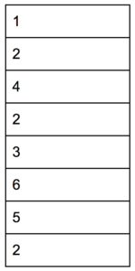
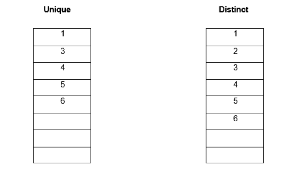
In this example, you have a list of numbers ranging from 1-6. The unique values are the ones that appear only once in the list, without any duplications. The distinct values are all the different values in the list. The tables below show the unique and distinct values in this list.
Count unique values in Excel
You can use the combination of the SUM and COUNTIF functions to count unique values in Excel. The syntax for this combined formula is = SUM(IF(1/COUNTIF(data, data)=1,1,0)). Here the COUNTIF formula counts the number of times each value in the range appears.
The resulting array looks like {1;2;1;1;1;1}. In the next step, you divide 1 by the resulting values. The IF function implements the logic such that if the values appear only once in the range, this step will generate 1, otherwise it will be a fraction value. The SUM function then sums all the values and returns the result. This is an array formula, so you have to assign it using Ctrl + Shift + Enter.
The following example contains a list of automobile products with their product ID and Names. You will count the unique items in this example.
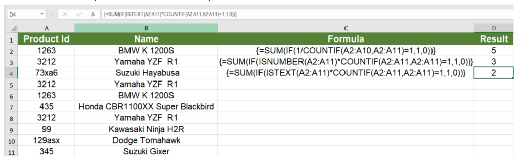
{=SUM(IF(1/COUNTIF(A2:A11,A2:A11)=1,1,0))}
This counts the number of unique values in the list. It follows the syntax mentioned above and returns the count for unique items, which is 5.
{=SUM(IF(ISNUMBER(A2:A11)*COUNTIF(A2:A11,A2:A11)=1,1,0))}
This counts the number of unique numeric values in the list. The only difference with the previous formula is here is the nested ISNUMBER formula that makes sure that you only count the numeric values. Returns the number 3, which is the count of the unique numeric values.
{=SUM(IF(ISTEXT(A2:A10)*COUNTIF(A2:A11,A2:A11)=1,1,0))}
Works the same as the previous formula, counts the unique number of text values instead. The ISTEXT function is used to make sure that only the text values are counted. Returns the number 2.
Count Distinct Values in Excel
Count Distinct Values using a Filter
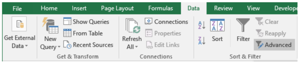
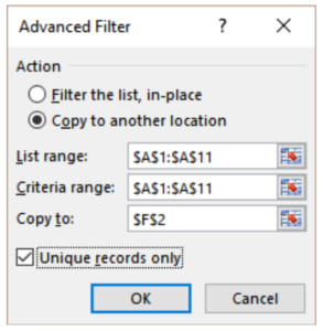
You can extract the distinct values from a list using the Advanced Filter dialog box and use the ROWS function to count the unique values. To count the distinct values from the previous example:
- Select the range of cells A1:A11.
- Go to Data > Sort & Filter > Advanced.
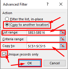
- In the Advanced Filter dialog box, click Copy to another location.
- Set both List Range and Criteria Range to $A$1:$A$11.
- Set Copy to to $F$2.
- Keep the Unique Records Only box checked. Click OK.
- Column F will now contain the distinct values.
- Select H6.
- Enter the formula
=ROWS(F3:F9). Click Enter.
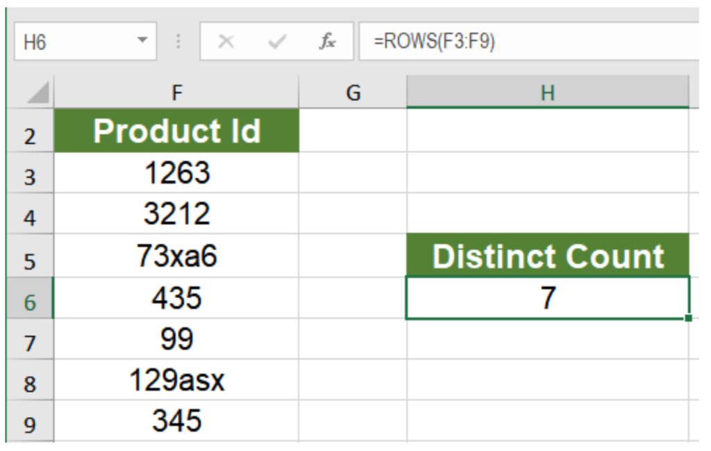
This will show the count of distinct values, 7.
Count Distinct Values using Formulas
You can use the combination of the IF, MATCH, LEN and FREQUENCY functions with the SUM function to count distinct values.
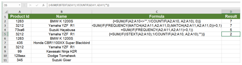
{=SUM(IF(A2:A11<>"",1/COUNTIF(A2:A11, A2:A11), 0))}
Counts the number of distinct values between cells A2 to A11. Like the unique count, here the COUNTIF function returns a count for each individual value which is then used as a denominator to divide 1. The returning values are then summed if they are not 0. This gives you a count for the distinct values, regardless of their types.
=SUM(IF(FREQUENCY(MATCH(A2:A11,A2:A11,0),MATCH(A2:A11,A2:A11,0))>0,1))
Does the same thing as the previous formula. The only differences being the use of the FREQUENCY and MATCH functions. The frequency function returns the number of occurrences for a value for the first occurrence. For the next occurrence of that value, it returns 0. The MATCH function is used to return the position of a text value in the range. These are returned as then used as an argument to the FREQUENCY function which gives us a count of the total number of distinct values.
=SUM(IF(FREQUENCY(A2:A11,A2:A11)>0,1))
Counts the number of distinct numeric values. As the FREQUENCY function ignores text and blanks, it returns 5, which is the number of numeric values.
{=SUM(IF(ISTEXT(A2:A11),1/COUNTIF(A2:A11, A2:A11),""))}
Returns the count of distinct text values in a range. Like the first example, this counts the distinct values, but the ISTEXT function makes sure only the text values are taken into count.
Count Distinct Values using a Pivot Table
You can also count distinct values in Excel using a pivot table. To find the distinct count of the bike names from the previous example:
To count the distinct items using a pivot table:
- Select cells A1:B11. Go to Insert > Pivot Table.
- In the dialog box that pops up, check New Worksheet and Add this to the Data Model.
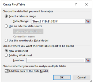
- Drag the Product ID field to Rows, Names field to Values in the PivotTable Fields.
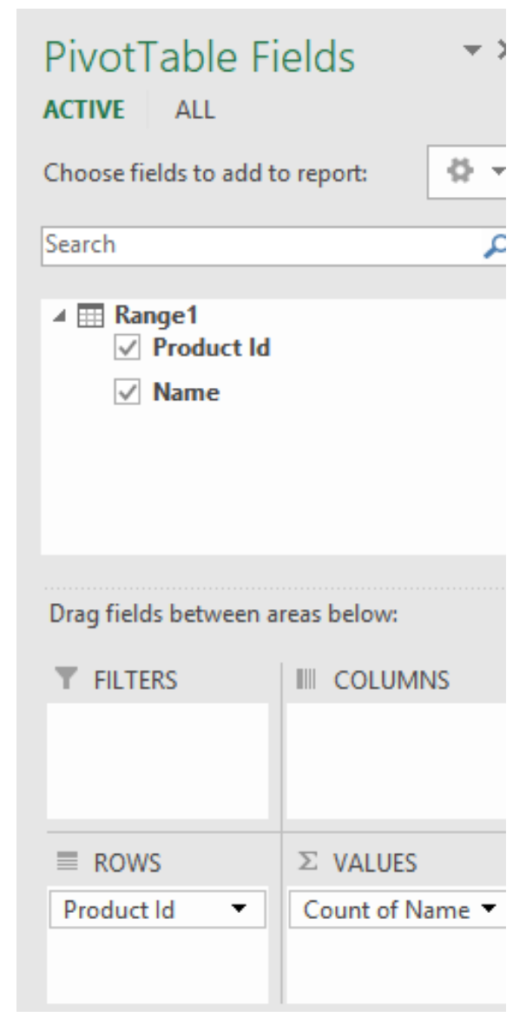
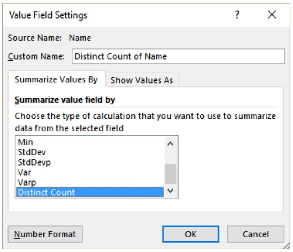
- Right-click on any value in column B. Go to Value Field Settings. In the Summarize Values By tab, go to Summarize Value field by and set it to Distinct Count.
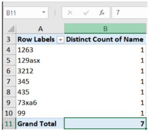
This will show the distinct count 7 in cell B11.
Still need some help with Excel formatting or have other questions about Excel? Connect with a live Excel expert here for some 1 on 1 help. Your first session is always free.
Skip to content
В этом руководстве вы узнаете, как посчитать уникальные значения в Excel с помощью формул и как это сделать в сводной таблице. Мы также разберём несколько примеров счёта уникальных текстовых и числовых значений, в том числе с учетом регистра букв.
При работе с большим набором данных в Excel вам часто может потребоваться знать, сколько в вашей таблице повторяющихся и сколько уникальных записей.
И вот о чем мы сейчас поговорим:
- Как посчитать уникальные значения в столбце.
- Считаем уникальные текстовые значения.
- Подсчет уникальных чисел.
- Как посчитать уникальные с учётом регистра.
- Формулы для подсчета различных значений.
- Как не учитывать пустые ячейки?
- Сколько встречается различных чисел?
- Считаем различные текстовые значения.
- Как сосчитать различные текстовые значения с учетом условий?
- Считаем количество различных чисел с ограничениями.
- Как учесть регистр при подсчёте?
- Как посчитать уникальные строки?
- Используем сводную таблицу.
Если вы регулярно посещаете этот блог, вы уже знаете формулу Excel для подсчета дубликатов. А сегодня мы собираемся изучить различные способы подсчета уникальных значений в Excel. Но для ясности давайте сначала определимся с терминами.
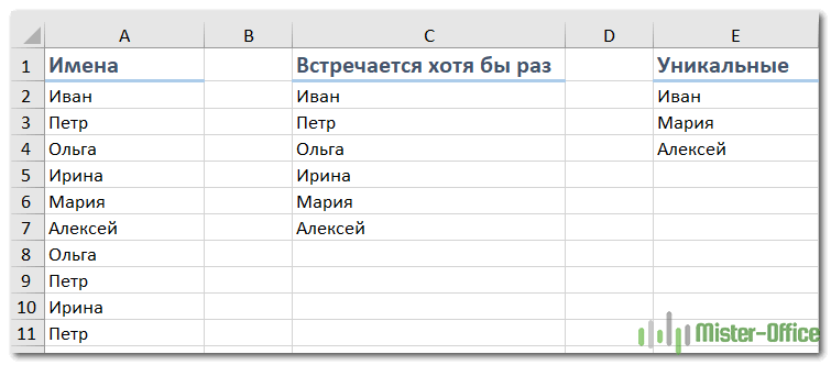
- Уникальные значения – те, которые появляются в списке только один раз.
- Различные – это все, которые имеются в списке без учета повторов, то есть уникальные плюс первое вхождение повторяющихся.
Следующий рисунок иллюстрирует эту разницу:
А теперь давайте посмотрим, как можно их посчитать с помощью формул и функций сводной таблицы.
Далее вы найдете несколько примеров для подсчета уникальных данных разных типов.
Считаем уникальные значения в столбце.
Предположим, у вас есть столбец с именами на листе Excel, и вам нужно подсчитать, сколько там есть неповторяющихся. Самое простое решение состоит в том, чтобы использовать функцию СУММ в сочетании с ЕСЛИ и СЧЁТЕСЛИ :
=СУММ(ЕСЛИ(СЧЁТЕСЛИ(диапазон ; диапазон ) = 1,1,0))
Примечание. Это формула массива, поэтому обязательно нажмите Ctrl + Shift + Enter, чтобы корректно ввести её. Как только вы это сделаете, Excel автоматически заключит всё выражение в {фигурные скобки}, как показано на скриншоте ниже. Ни в коем случае нельзя вводить фигурные скобки вручную, это не сработает.
В этом примере мы считаем уникальные имена в диапазоне A2: A10, поэтому наше выражение выглядит так:
{=СУММ(ЕСЛИ(СЧЁТЕСЛИ(A2:A10;A2:A10)=1;1;0))}

Этот метод подходит и для текстовых, и для цифровых данных. Недостатком является то, что в качестве уникального он будет пересчитывать любое содержимое, в том числе и ошибки.
Далее в этом руководстве мы обсудим несколько других подходов для подсчета уникальных значений разных типов. И поскольку в основном они являются вариациями этой базовой формулы, имеет смысл подробно рассмотреть её. Если вы поймете, как это работает, то сможете настроить ее для своих данных. Если кого-то не интересуют технические подробности, вы можете сразу перейти к следующему примеру.
Как работает формула подсчета уникальных значений?
Как видите, здесь используются 3 разные функции – СУММ, ЕСЛИ и СЧЁТЕСЛИ. Посмотрим, что делает каждая из них:
- Функция СЧЁТЕСЛИ считает, сколько раз каждое отдельное значение появляется в анализируемом диапазоне.
В этом примере СЧЁТЕСЛИ(A2:A10;A2:A10)возвращает массив {3:2:2:1:1:2:3:2:3}.
- Функция ЕСЛИ оценивает каждый элемент в этом массиве, сохраняет все единицы (то есть, уникальные) и заменяет все остальные цифры нулями.
Итак, функция ЕСЛИ(СЧЁТЕСЛИ(A2:A10;A2:A10)=1;1;0) преобразуется в ЕСЛИ({3:2:2:1:1:2:3:2:3}) = 1,1,0).
И далее она превращается в массив чисел {0:0:0:1:1:0:0:0:0}. Здесь 1 означает уникальное значение, а 0 – появляющееся более 1 раза.
- Наконец, функция СУММ складывает числа в этом итоговом массиве и выводит общее количество уникальных значений. Что нам и нужно.
Подсчет уникальных текстовых значений.
Если ваш список содержит как числа так и текст, и вы хотите посчитать только уникальные текстовые строки, добавьте функцию ЕТЕКСТ() в формулу массива, описанную выше:
{=СУММ(ЕСЛИ(ЕТЕКСТ(A2:A10)*СЧЁТЕСЛИ(A2:A10;A2:A10)=1;1;0))}
Функция ЕТЕКСТ возвращает ИСТИНА, если исследуемое содержимое ячейки является текстом, и ЛОЖЬ в противоположном случае. Поскольку звездочка (*) в формулах массива работает как оператор И, то функция ЕСЛИ возвращает 1, только если рассматриваемое одновременно текстовое и уникальное, в противном случае получаем 0. И после того, как функция СУММ сложит все числа, вы получите количество уникальных текстовых значений в указанном диапазоне.
Не забывайте нажимать Ctrl + Shift + Enter, чтобы правильно ввести формулу массива, и вы получите результат, подобный этому:

Рис3
Как вы можете видеть на скриншоте выше, мы получили общее количество уникальных текстовых значений, исключая пустые ячейки, числа, логические выражения ИСТИНА и ЛОЖЬ, а также ошибки.
Как сосчитать уникальные числовые значения.
Чтобы посчитать уникальные числа в списке данных, используйте формулу массива точно так же, как мы только что делали при подсчете текстовых данных. Отличие заключается в том, что вы используете ЕЧИСЛО вместо ЕТЕКСТ:
{=СУММ(ЕСЛИ(ЕЧИСЛО(A2:A10)*СЧЁТЕСЛИ(A2:A10;A2:A10)=1;1;0))}
Пример и результат вы видите на скриншоте чуть выше.
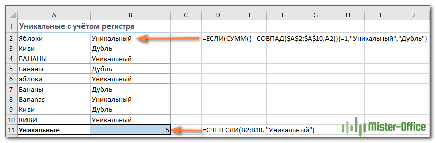
Уникальные значения с учетом регистра.
Если для вас принципиально различие в заглавных и прописных буквах, то самым простым способом подсчета будет создание вспомогательного столбца со следующей формулой массива для идентификации повторяющихся и уникальных элементов:
{=ЕСЛИ(СУММ((—СОВПАД($A$2:$A$10;A2)))=1;»Уникальный»;»Дубль»)}
А затем используйте простую функцию СЧЁТЕСЛИ для подсчета уникальных значений:
=СЧЁТЕСЛИ(B2:B10; «Уникальный»)
А теперь посмотрим, как можно посчитать количество значений, которые появляются хотя бы один раз, то есть так называемых различных значений.
Подсчет различных значений.
Используйте следующую универсальное выражение:
{=СУММ(1 / СЧЁТЕСЛИ( диапазон ; диапазон ))}
Помните, что это формула массива, поэтому вам следует нажать Ctrl + Shift + Enter, вместо обычного Enter.
Кроме того, вы можете использовать функцию СУММПРОИЗВ и записать формулу обычным способом:
=СУММПРОИЗВ(1 / СЧЁТЕСЛИ( диапазон ; диапазон ))
Например, чтобы сосчитать различные значения в диапазоне A2: A10, вы можете использовать выражение:
{=СУММ(1/СЧЁТЕСЛИ(A2:A10;A2:A10))}
или же
=СУММПРОИЗВ(1/СЧЁТЕСЛИ(A2:A10;A2:A10))

Этот способ подходит не только для подсчета в столбце, но и для диапазона данных. К примеру, у нас под имена отведено две колонки. Тогда делаем так:
{=СУММПРОИЗВ(1/СЧЁТЕСЛИ(A2:B10;A2:B10))}
Этот метод подходит для текста, чисел, дат.
Единственное ограничение – диапазон должен быть непрерывным и не содержать пустых ячеек и ошибок.
Если в вашем диапазоне данных есть пустые ячейки, то можно изменить:
{=СУММПРОИЗВ(1/СЧЁТЕСЛИ(A2:A10; A2:A10&»»))}
Тогда в расчёт попадёт и будет засчитана и пустая ячейка.
Как это работает?
Как вы уже знаете, мы используем функцию СЧЁТЕСЛИ, чтобы узнать, сколько раз каждый отдельный элемент встречается в указанном диапазоне. В приведенном выше примере, результат работы функции СЧЕТЕСЛИ представляет собой числовой массив: {3:2:2:1:3:2:1:2:3}.
После этого выполняется ряд операций деления, где единица делится на каждую цифру из этого массива. Это превращает все неуникальные значения в дробные числа, соответствующие количеству повторов. Например, если число или текст появляется в списке 2 раза, в массиве создаются 2 элемента равные 0,5 (1/2 = 0,5). А если появляется 3 раза, в массиве создаются 3 элемента 0,333333.
В нашем примере результатом вычисления выражения 1/СЧЁТЕСЛИ(A2:A10;A2:A10) является массив {0.333333333333333:0.5:0.5:1:0.333333333333333:0.5:1:0.5:0.333333333333333}.
Пока не слишком понятно? Это потому, что мы еще не применили функцию СУММ / СУММПРОИЗВ. Когда одна из этих функций складывает числа в массиве, сумма всех дробных чисел для каждого отдельного элемента всегда дает 1, независимо от того, сколько раз он появлялся. И поскольку все уникальные элементы отображаются в массиве как единицы (1/1 = 1), окончательный результат представляет собой общее количество всех встречающихся значений.
Как и в случае подсчета уникальных значений в Excel, вы можете использовать варианты универсальной формулы для обработки отдельно чисел, текста или же с учетом регистра.
Помните, что все приведенные ниже выражения являются формулами массива и требуют нажатия Ctrl + Shift + Enter.
Подсчет различных значений без учета пустых ячеек
Если столбец, в котором вы хотите совершить подсчет, может содержать пустые ячейки, вам следует в уже знакомую нам формулу массива добавить функцию ЕСЛИ. Она будет проверять ячейки на наличие пустот (основная формула Excel, описанная выше, в этом случае вернет ошибку #ДЕЛ/0):
=СУММ(ЕСЛИ( диапазон <> «»; 1 / СЧЁТЕСЛИ( диапазон ; диапазон ); 0))
Вот как, к примеру, можно посчитать количество индивидуальных значений, игнорируя пустые ячейки:

Используем:
{=СУММ(ЕСЛИ(A2:A10<>»»;1/СЧЁТЕСЛИ(A2:A10; A2:A10); 0))}
Как видите, наш список состоит из трёх имён.
Подсчет различных чисел.
Чтобы посчитать различные числовые значения (числа, даты и время), используйте функцию ЕЧИСЛО:
= СУММ(ЕСЛИ(ЕЧИСЛО( диапазон ); 1 / СЧЁТЕСЛИ( диапазон ; диапазон ); «»))
Считаем, сколько имеется различных чисел в диапазоне A2: A10:
{=СУММ(ЕСЛИ(ЕЧИСЛО(A2:A10);1/СЧЁТЕСЛИ(A2:A10; A2:A10);»»))}
Результат вы можете посмотреть ниже.

Это достаточно простое и элегантное решение, но работает оно гораздо медленнее, чем выражения, которые используют функцию ЧАСТОТА для подсчета уникальных значений. Если у вас большие наборы данных, то целесообразно переключиться на формулу, основанную на расчёте частот.
И вот еще один способ подсчета чисел:
=СУММ(—(ЧАСТОТА(диапазон; диапазон)>0))
Применительно к примеру ниже:
=СУММ(—(ЧАСТОТА(A2:A10; A2:A10)>0))
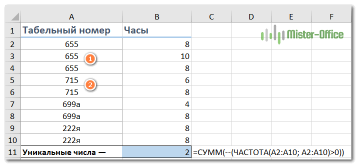
Как видите, здесь игнорируются записи, в которых имеются буквы.
Пошагово разберём, как это работает.
Функция ЧАСТОТА возвращает массив цифр, которые соответствуют интервалам, заданным имеющимися числами. В этом случае мы сравниваем один и тот же набор чисел для массива данных и для массива интервалов.
Результатом является то, что ЧАСТОТА() возвращает массив, который представляет собой счетчик для каждого числового значения в массиве данных.
Это работает, потому что ЧАСТОТА() возвращает ноль для любых чисел, которые ранее уже появились в списке. Ноль возвращается и для текстовых данных. Поэтому полученный массив выглядит следующим образом:
{3:0:0:2:0:0}
Как видите, обрабатываются только числа. Ячейки A7:A10 игнорируются, потому что там текст. А функция ЧАСТОТА() работает только с числами.
Теперь каждое из этих чисел проверяем на условие «больше нуля».
Получаем:
{ИСТИНА:ЛОЖЬ:ЛОЖЬ:ИСТИНА:ЛОЖЬ:ЛОЖЬ}
Теперь превращаем ИСТИНА и ЛОЖЬ в 1 и 0 соответственно. Делаем это при помощи двойного отрицания. Проще говоря, это двойной минус, который не меняет величину числа, но позволяет получить реальные числа, когда это вообще возможно:
{1:0:0:1:0:0}
А теперь функция СУММ складывает всё и получаем результат: 2.
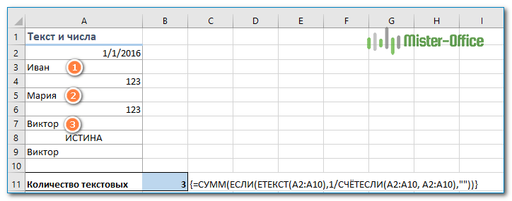
Различные текстовые значения.
Чтобы посчитать отдельные текстовые записи в столбце, мы будем использовать тот же подход, который мы использовали для исключения пустых ячеек.
Как вы можете легко догадаться, мы просто добавим функцию ЕТЕКСТ и проверку условия:
=СУММ(ЕСЛИ(ЕТЕКСТ( диапазон ); 1 / СЧЁТЕСЛИ( диапазон ; диапазон ); «»))
Количество индивидуальных символьных значений посчитаем так:
{=СУММ(ЕСЛИ(ЕТЕКСТ(A2:A10);1/СЧЁТЕСЛИ(A2:A10; A2:A10);»»))}
Не забываем, что это формула массива.
Если в вашей таблице нет пустых ячеек и ошибок, то вы можете применить формулу, которая использует несколько функций: ЧАСТОТА, ПОИСКПОЗ, СТРОКА и СУММПРОИЗВ.
В общем виде это выглядит так:
=СУММПРОИЗВ(—(ЧАСТОТА(ПОИСКПОЗ (диапазон; диапазон;0); СТРОКА (диапазон)- СТРОКА (диапазон_первая_ячейка)+1)>0))
Предположим, у вас есть список имен сотрудников вместе с часами работы над проектом, и вы хотите знать, сколько человек в этом участвовали. Глядя на данные, вы можете увидеть, что имена повторяются. А вы хотите пересчитать всех, кто хотя бы раз появился в этом списке.

Применяем формулу массива:
{=СУММПРОИЗВ(— (ЧАСТОТА(ПОИСКПОЗ(A2:A10; A2:A10;0); СТРОКА(A2:A10) -СТРОКА(A2) +1)> 0))}
Она является более сложной, чем аналогичная, которая использует функцию ЧАСТОТА() для подсчета различных чисел. Это потому, что ЧАСТОТА() не работает с текстом. Поэтому ПОИСКПОЗ преобразует имена в номера позиций, которые может обрабатывать ЧАСТОТА().
Если какая-либо из ячеек в диапазоне пустая, вам необходимо использовать более сложную формулу массива, которая включает в себя функцию ЕСЛИ:
{= СУММ(ЕСЛИ(ЧАСТОТА(ЕСЛИ(данные <> «»;ПОИСКПОЗ(данные; данные; 0));СТРОКА(данные) -СТРОКА(данные_первая_ячейка) +1); 1))}
Примечание: поскольку логическая проверка в операторе ЕСЛИ содержит массив, то наше выражение сразу становится формулой массива, которая требует ввода через Ctrl+Shift+Enter. Поэтому же СУММПРОИЗВ была заменена на СУММ.
Применительно к нашему примеру это выглядит так:
{=СУММ(ЕСЛИ(ЧАСТОТА(ЕСЛИ(A2:A10 <> «»;ПОИСКПОЗ(A2:A10; A2:A10; 0));СТРОКА(A2:A10) -СТРОКА(A2) +1); 1))}
Теперь «сломать» этот расчет может только наличие ячеек с ошибками в исследуемом диапазоне.
Различные текстовые значения с условием.
Предположим, необходимо пересчитать, сколько наименований товаров заказал конкретный покупатель.
Чтобы решить эту проблему, вам может помочь этот вариант:
{=СУММПРОИЗВ((($A$2:$A$18=E2)) / СЧЁТЕСЛИМН($A$2:$A$18;$A$2:$A$18&»»; $B$2:$B$18;$B$2:$B$18&»»))}
Введите это в пустую ячейку, куда вы хотите поместить результат, F2, например. А затем нажмите Shift + Ctrl + Enter вместе, чтобы получить правильный результат.
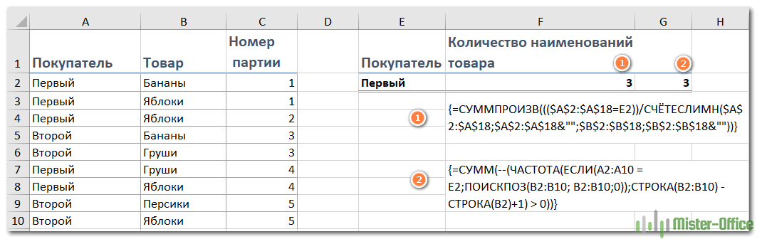
Поясним: здесь A2:A18 это список покупателей, с учётом которого вы ограничиваете область расчётов, B2: B18 — перечень товаров, в котором вы хотите посчитать уникальные значения, Е2 содержит критерий, на основании которого подсчет ограничивается только конкретным покупателем.
Второй способ.
Для уникальных значений в диапазоне с критериями, вы можете использовать формулу массива, основанную на функции ЧАСТОТА.
{=СУММ(—(ЧАСТОТА(ЕСЛИ(критерий; ПОИСКПОЗ(диапазон; диапазон;0)); СТРОКА(диапазон) -СТРОКА(диапазон_первая_ячейкаl)+1)>0))}
Применительно к нашему примеру:
{=СУММ(—(ЧАСТОТА(ЕСЛИ(A2:A10 = E2; ПОИСКПОЗ(B2:B10; B2:B10;0)); СТРОКА(B2:B10) — СТРОКА(B2)+1) > 0))}
С учетом ограничений ЕСЛИ() функция ПОИСКПОЗ определяет порядковый номер только для строк, которые соответствуют критериям.
Если какая-либо из ячеек в диапазоне критериев пустая, вам необходимо скорректировать расчёт, добавив дополнительно ЕСЛИ для обработки пустых ячеек. Иначе они будут переданы в функцию ПОИСКПОЗ, которая в ответ сгенерирует сообщение об ошибке.
Вот что получилось после корректировки:
{=СУММ(— (ЧАСТОТА(ЕСЛИ(B2:B10 <> «»; ЕСЛИ(A2:A10 = E2; ПОИСКПОЗ(B2:B10; B2:B10;0))); СТРОКА(B2:B10) -СТРОКА(B2) +1)> 0))}
То есть все действия и расчёты мы производим, если в столбце B нам встретилась непустая ячейка: ЕСЛИ(B2:B10 <> «»….
Если у вас есть два критерия, вы можете расширить логику формулы путем добавления другого вложенного ЕСЛИ.
Поясним. Определим, сколько наименований товара находилось в первой партии первого покупателя.
Критерии запишем в G2 и G3.
В общем виде это выглядит так:
{=СУММ(—(ЧАСТОТА(ЕСЛИ(критерий1; ЕСЛИ(критерий2; ПОИСКПОЗ (диапазон; диапазон;0))); СТРОКА (диапазон) — СТРОКА (диапазон_первая_позиция) +1)> 0))}
Подставляем сюда реальные данные и получаем результат:

{=СУММ(—(ЧАСТОТА(ЕСЛИ(A2:A10=G2; ЕСЛИ(C2:C10=G3;ПОИСКПОЗ(B2:B10;B2:B10;0)));СТРОКА(B2:B10)-СТРОКА(B2)+1)>0))}
В первой партии 2 наименования товара, хотя и 3 позиции.
Различные числа с условием.
Если вам нужно пересчитать уникальные (с учётом первого вхождения) числа в диапазоне с учетом каких-то ограничений, можно использовать формулу, основанную на СУММ и ЧАСТОТА, и вместе с этим применять критерии.
{=СУММ(— (ЧАСТОТА(ЕСЛИ(критерий; диапазон); диапазон)> 0))}
Предположим, у нас есть перечень табельных номеров и количество отработанных часов по дням. Нужно сосчитать, сколько человек хотя бы раз отработали менее чем по 8 часов, то есть неполную смену.

Вот наша формула массива:
{=СУММ(— (ЧАСТОТА(ЕСЛИ(B2:B10 < 8; A2:A10); A2:A10)> 0))}
Как видите, таких случаев 3, но связаны они с двумя работниками.
Различные значения с учетом регистра.
Подобно подсчету уникальных, самый простой способ подсчета различных значений с учетом регистра – это добавить вспомогательный столбец с формулой массива, который идентифицирует нужные элементы, включая первые повторяющиеся вхождения.
Подход в основном такой же, как и тот, который мы использовали для подсчета уникальных значений с учетом регистра, с одним небольшим изменением:
{=ЕСЛИ(СУММ((—СОВПАД($A$2:$A2;$A2)))=1;»Уникальный»;»»)}
Как вы помните, все формулы массива в Excel требуют нажатия Ctrl + Shift + Enter.
После того, как это выражение будет записано, вы можете посчитать «различные» значения с помощью обычной функции СЧЁТЕСЛИ, например:
=СЧЁТЕСЛИ(B2:B10; «Уникальный»)
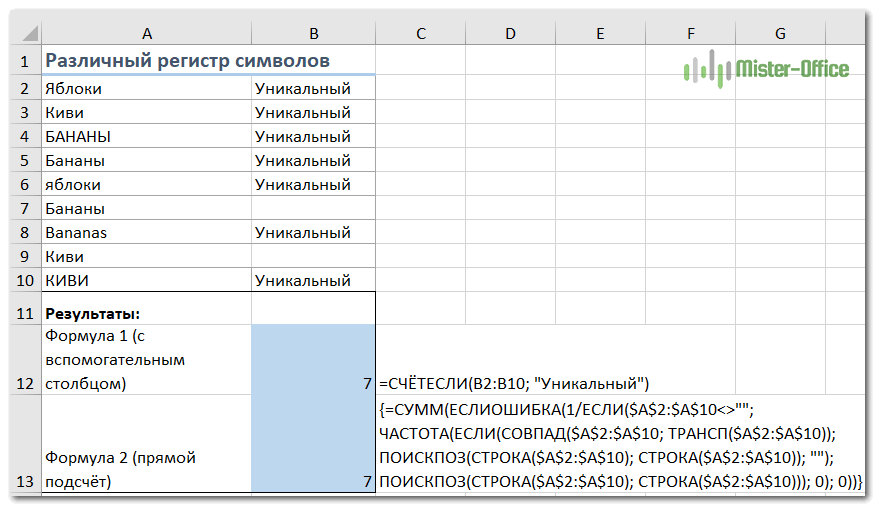
Если вы не можете добавить вспомогательный столбец на свой рабочий лист, вы можете использовать следующую более сложную формулу массива для подсчета различных значений с учетом регистра без создания дополнительного столбца:
{=СУММ(ЕСЛИОШИБКА(1/ЕСЛИ($A$2:$A$10<>»»; ЧАСТОТА(ЕСЛИ(СОВПАД($A$2:$A$10; ТРАНСП($A$2:$A$10)); ПОИСКПОЗ(СТРОКА($A$2:$A$10); СТРОКА($A$2:$A$10)); «»); ПОИСКПОЗ(СТРОКА($A$2:$A$10); СТРОКА($A$2:$A$10))); 0); 0))}
Как видите, обе формулы дают одинаковые результаты.
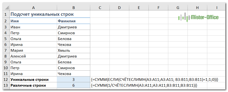
Подсчет уникальных строк в таблице.
Подсчет уникальных / различных строк в Excel сродни пересчёту уникальных и различных значений. С той лишь разницей, что вы используете функцию СЧЁТЕСЛИМН вместо СЧЁТЕСЛИ, что позволяет вам указать сразу несколько столбцов для проверки уникальности.
Например, чтобы подсчитать уникальные строки на основе столбцов A (Имя) и B (Фамилия), используйте один из следующих вариантов:
Для уникальных строк:
{=СУММ(ЕСЛИ(СЧЁТЕСЛИМН(A3:A11;A3:A11; B3:B11;B3:B11)=1;1;0))}
Для различных строк:
{=СУММ(1/СЧЁТЕСЛИМН(A3:A11;A3:A11;B3:B11;B3:B11))}
Естественно, вы не ограничены только двумя столбцами. Функция СЧЁТЕСЛИМН может обрабатывать до 127 пар диапазон / критерий.
Как можно использовать сводную таблицу.
Вот обычная задача, которую все пользователи Excel должны время от времени выполнять. У вас есть список данных (к примеру, названий товаров), и нужно узнать количество уникальных позиций в этом списке. Как это сделать? Проще, чем вы думаете 
В версиях Excel выше 2013 есть специальная функция, которая позволяет автоматически пересчитывать различные значения в сводной таблице. На следующем рисунке показано, как выглядит этот счетчик:

Чтобы создать сводную таблицу со счетчиком для определенного столбца, выполните следующие действия.
- Выберите данные для включения в сводную таблицу, перейдите на вкладку «Вставка» и нажмите кнопку «Сводная таблица» .
- В диалоговом окне «Создание сводной таблицы» выберите, следует ли разместить сводную таблицу на новом или существующем листе, и обязательно установите флажок «Добавить эти данные в модель данных» .

- Когда откроется сводная таблица, расположите области строк, столбцов и значений так, как вам нужно. Если у вас нет большого опыта работы со сводными таблицами Excel, могут оказаться полезными следующие подробные рекомендации: Создание сводной таблицы в Excel.
- Переместите поле, количество уникальных элементов которого вы хотите вычислить ( поле « Товар» в этом примере), в область « Значения» , щелкните его и выберите «Параметры значения поля…» из раскрывающегося меню.
- Откроется диалоговое окно , прокрутите вниз до операции «Число разных элементов» , которая является самым последним пунктом в списке, выберите ее и нажмите OK .
Вы также можете дать собственное имя своему счетчику, если хотите.

Готово! Вновь созданная сводная таблица будет отображать количество различных товаров, как показано на самом первом скриншоте в этом разделе.
Вот как можно подсчитать различные и уникальные значения в столбце и целиком в таблице Excel.
Благодарю вас за чтение и надеюсь увидеть вас снова. Пожалуйста, не переключайтесь!
 Как найти и выделить уникальные значения в столбце — В статье описаны наиболее эффективные способы поиска, фильтрации и выделения уникальных значений в Excel. Ранее мы рассмотрели различные способы подсчета уникальных значений в Excel. Но иногда вам может понадобиться только просмотреть уникальные…
  Как получить список уникальных значений — В статье описано, как получить список уникальных значений в столбце с помощью формулы и как настроить эту формулу для различных наборов данных. Вы также узнаете, как быстро получить отдельный список с…
  Как выделить цветом повторяющиеся значения в Excel? — В этом руководстве вы узнаете, как отображать дубликаты в Excel. Мы рассмотрим различные методы затенения дублирующих ячеек, целых строк или последовательных повторений с использованием условного форматирования. Ранее мы исследовали различные…
  Как посчитать количество повторяющихся значений в Excel? — Зачем считать дубликаты? Мы можем получить ответ на множество интересных вопросов. К примеру, сколько клиентов сделало покупки, сколько менеджеров занималось продажей, сколько раз работали с определённым поставщиком и т.д. Если…
  Как убрать повторяющиеся значения в Excel? — В этом руководстве объясняется, как удалять повторяющиеся значения в Excel. Вы изучите несколько различных методов поиска и удаления дубликатов, избавитесь от дублирующих строк, обнаружите точные повторы и частичные совпадения. Хотя…
Do you want to count distinct values in a list in Excel?
When performing any data analysis in Excel you will often want to know the number of distinct items in a column. This statistic can give you a useful overview of the data and help you spot errors or inconsistencies.
This post will show you all the ways you can count the number of distinct items in your list. Get your copy of the example workbook in this post to follow along.
Distinct vs Unique
The terms unique and distinct are often incorrectly interchanged liberally. There is a big difference between these terms.
Distinct means values that are different. The distinct values from this list {A, B, B, C} are {A, B, C}. The count in this case will be 3.
Unique means values that only appear once. The unique values from the list {A, B, B, C} are {A, C}. The count in this case will be 2.
💡 Tip: Check out this post if you are actually looking for a count of unique items.
Count Distinct Values with the COUNTIFS Function
The first way to count the unique values in a range is with the COUNTIFS function.
The COUNTIFS function allows you to count values based on one or more criteria.
= SUM ( 1 / COUNTIFS ( B5:B14, B5:B14 ) )The above formula will count the number of distinct items from the list of values in the range B5:B14.
The COUNTIFS function is used to see how many times each value appears in the list. When you invert this count you get a fractional value that will add up to 1 for each distinct value in the list.
The SUM function then adds all these fractions up and the total is the number of distinct items in the list.
💡 Tip: If you are working with an older version of Excel that doesn’t support array formulas, then you will need to enter this formula with Ctrl + Shift + Enter.
Count Distinct Values with the UNIQUE Function
Another formula approach to counting the number of distinct items from the list is with dynamic array functions.
However, these are only available in Excel for Microsoft 365.
= COUNTA ( UNIQUE ( B5:B14 ) )The above formula will return the count of all distinct items from the list in B5:B14.
The UNIQUE function returns all the distinct values from the list. The number of items in the distinct list is then counted using the COUNTA function.
Count Distinct Values with Advanced Filters
Advanced Filters is a feature that allows you to add complex logic based on multiple fields to filter your lists.
This can also be used to filter the distinct values in your list.
You can then use a SUBTOTAL function to count only the visible items in your filtered list.
Here’s how to count the distinct items with the advanced filters.
= SUBTOTAL ( 103, B5:B14 )- Add the above SUBTOTAL function to the range you want to count values from. The
103argument tells the SUBTOTAL function to only count the visible cells in a range.
- Select the column of data in which you want to count distinct values.
- Go to the Data tab.
- Click on the Advanced command in the Sort and Filter section of the ribbon.
This will open the Advanced Filter menu.
- Select the Filter the list in place option from the Action section.
- The List range should be the range of values previously selected in step 2. You can update this if needed.
- Check the Unique records only option. Even though it says unique, it will actually return the distinct values in the filter.
- Press the OK button.
The list is filtered to hide all the repeated values and the SUBTOTAL will then only count the distinct items in the list.
Count Distinct Values with a Pivot Table
You can get a list of distinct values from a pivot table.
When you summarize your data by rows in a pivot table, the rows area will show only the distinct items. You can then count these with the status bar statistics or the COUNTA function.
You will first need to create a pivot table with the data that you want to get a distinct count.
- Select the data.
- Go to the Insert tab.
- Click on the PivotTable command.
This opens the PivotTable from table or range menu where you can select where you want to place the new pivot table.
- Choose the location for your new pivot table.
- Press the OK button.
This will create a new blank pivot table. When you select any cell inside this pivot table, you will see the PivotTable Fields list appear on the right side of the workbook.
- Drag the field from which you want to count distinct items into the Rows area of the pivot table.
This creates a list of distinct items in the pivot table. Now you can select these items and the count will be displayed in the status bar area.
Count Distinct Values with the Pivot Table Data Model
While using a pivot table will get you the list of distinct items from your data, it’s not ideal for counting the results. There is an additional step of selecting the items and getting the count in the status bar.
But there is a way to use a pivot table and return the count of distinct items inside the Values area of the pivot table.
When you use the pivot table data model feature, it will reveal an extra summary type in the field settings that will count distinct values.
You will insert the pivot table as before, but there is an extra step during the process.
- Check the Add this data to the Data Model option in the PivotTable from table or range menu.
- Drag the field into the Values area. It should default to a count.
- Left-click on the field.
- Select Value Field Settings from the menu options.
This opens the Value Field Settings menu.
- Go to the Summarize Values By tab.
- Choose the Distinct Count option in the Summarize value field by list. This option only appears when the data has been added to the data model.
- Press the OK button.
That’s it! The distinct count of items now appears in your pivot table.
This is much more versatile as you can now get the distinct count within another categorical grouping by adding a field into the Rows area.
For example, each value in the pivot table is now a distinct count of the car model based on the make.
Count Distinct Values Remove Duplicates
The Remove Duplicates feature will allow you to get rid of any repeated values in your list.
You can then count the results to get a distinct count of items.
- Select the range of items to count.
- Go to the Data tab.
- Click on the Remove Duplicates command.
This will open the Remove Duplicates menu.
- Select a single column in the list of Columns.
- Press the OK button.
This will remove the duplicates in your list and a popup will show telling you how many items were removed and how many remain. This is the number of distinct items from the list!
📝 Note: This will change the data, so be sure to only perform this command on a copy of your source data so you don’t lose the original.
Count Distinct Values with Power Query Column Distribution
Power Query is a great tool for importing and transforming data.
When building your queries, it will even show you useful summary statistics about the data in the column distribution view. This includes a distinct count.
You will first need to load your data into the Power Query editor to see these features.
- Select the data.
- Go to the Data tab.
- Select the From Table/Range query option.
This will open the Power Query editor and you might already see the column distribution feature with the distinct count.
If you don’t see this, you can enable it from the View tab in the editor.
- Go to the View tab.
- Check the Column distribution option in the Data Preview section.
💡 Tip: Hover your mouse cursor over the counts and you’ll see a percentage distribution!
Count Distinct Values with Power Query Transform Tab
The column distribution feature is handy for a quick overview of the data, but you might want to get this value back into Excel from your Power Query.
This is also possible.
- Select the column you want to count.
- Go to the Transform tab.
- Click on the Statistics command in the Number Column section.
- Select the Count Distinct Values option from the menu.
This returns a sing scalar value from your column which is the count of the distinct items in that column.
You can load this back into Excel and it will load into a single column and single row table. Go to the Home tab and click on the Close and Load button.
Count Distinct Values with VBA
There is no prebuilt function in Excel that will count the number of distinct items in a range.
However, you can build your own custom VBA function for this purpose.
Press the Alt + F11 keyboard shortcut to open the visual basic editor. This is where you can place the code for your user-defined function.
Go to the Insert menu and select the Module option to create a new module for your code.
Function COUNTDISTINCTVALUES(rng As Range) As Integer
Application.Volatile
Dim c As Variant
Dim distinctValues As New Collection

On Error Resume Next
For Each c In rng
    If Not (IsEmpty(c)) Then
        distinctValues.Add c, CStr(c)
    End If
Next c
COUNTDISTINCTVALUES = distinctValues.Count
End Function
Copy and paste the above code into the module.
This code will create a new function named COUNTDISTINCTVALUES which can be used anywhere in the workbook just like any other function.
The will loop through each cell in the range it is passed. If the cell is not empty, then the value in the cell is added to a collection object.
Collections will only allow distinct values to be added, so the end result will be a collection of only the distinct values from your range.
The count of the items in the collection is then returned as the function output!
= COUNTDISTINCTVALUES ( B3:B12 )The above formula will then return the distinct count of the values in the range B3:B12.
Count Distinct Values with Office Scripts
Office scripts are another way to get a distinct count for a selected range.
You can create a script that will count distinct items in the active range.
Go to the Automate tab and select the New Script option.
This will open the Code Editor.
function main(workbook: ExcelScript.Workbook) {
    let rng = workbook.getSelectedRange();
    let rngValues = rng.getValues();
    let arrayValues = rngValues.reduce((a, value) => a.concat(value), []);
    let distinctValues = new Set(arrayValues);
    console.log(distinctValues.size);
};
Add the above code and press the Save script button.
This code gets the values from the selected range in the sheet. It will then convert this to a one-dimensional array of values with the reduce function.
This 1D array is then added to a Set. Sets also have the property that they only allow distinct values, so the distinctValues set will only have the distinct values from the selected range.
The number of items is counted with the size and this is returned to the console log to give you the count of distinct values.
Conclusions
There are several options for counting the distinct number of items in a list.
Formulas solutions are great for dynamic live results directly in your sheet. Other features such as advanced filters or remove duplicates are only suited for one-time uses.
If you’re already using Pivot Tables or Power Query in your data processing, then getting the distinct count in those tools is a natural choice.
For any other situation, or as part of a larger automated process, the custom VBA or Office Scripts code solutions might be the best.
Did you know any of these methods? Let me know in the comments!
About the Author
John is a Microsoft MVP and qualified actuary with over 15 years of experience. He has worked in a variety of industries, including insurance, ad tech, and most recently Power Platform consulting. He is a keen problem solver and has a passion for using technology to make businesses more efficient.
Home > Microsoft Excel > How to Count Unique Values in Excel? 3 Easy Ways to Count Unique and Distinct Values
(Note: This guide on how to freeze rows in Excel is suitable for all Excel versions including Office 365)
Working with large amounts of data in Excel can be quite difficult. Some values may be repeated more than once. You might have to take into account multiple entries of data while performing any function to upgrade your accuracy. You will also need to count the values to organize or even acquire statistics from the data.
With large data, it would be nearly impossible to count the values manually. Especially, keeping a track of unique or distinct values can be quite arduous. Fortunately in Excel, there are many ways to count unique and distinct values.
You’ll Learn:
- Unique and Distinct Values
- How to Count Unique Values in Excel
- Using SUM, IF, and COUNTIF Functions
- Count Unique Text Values in Excel
- Count Unique Numeric Values in Excel
- Using SUM, IF, and COUNTIF Functions
- How to Count Distinct Values in Excel
- Using Filter Option
- Using SUM and COUNTIF functions
First, let us understand the difference between Unique and Distinct Values.
Unique and Distinct Values
Data can be repeated or unrepeated. These unrepeated data are of two types. They are called unique data and distinct data.
Unique data are those which occur in the dataset only once.
Whereas, distinct data include the duplicate values but count them only once.
I will explain unique and distinct data with an example for better understanding.
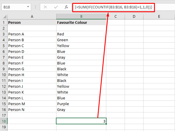
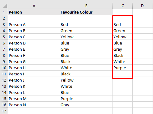
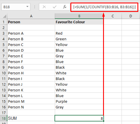
Consider an example, where column A has the list of people and column B lists their favorite colors.

In this, red, green, and purple colors occur only once, so they are called unique elements. Therefore the unique elements count is 3
Whereas, there are 8 distinct elements. That is the colors, though repeated are counted once. The colors are red, green, yellow, blue, white, black, gray, and purple. So, the distinct value count is 8.

In this guide, I will show you how to count unique and distinct values in Excel.
Let’s dive in.
How to Count Unique Values in Excel
First, let us see how to count unique values in excel.
Using SUM, IF, and COUNTIF Functions
In Excel, functions are always available to solve any operations. In this case, you can use a combination of SUM, IF and COUNTIF functions to count unique values in Excel.
To count unique values, enter the formula =SUM(IF(COUNTIF(range, range)=1,1,0)) in the desired cell. The range denotes the starting cell and the ending cell.
This is an array formula where the count values are stored in a new array. Since this is an array formula, make sure you press Ctrl+Shift+Enter after entering the formula. Also, note that when you enter the formula, curly braces will automatically populate at the end of them. But, do not enter them manually.
Consider the above example. To calculate the unique values in the given Excel sheet, enter the formula in the destination cell.
In the place of range, enter the cells which contain the elements whose unique value is to be found. Here, cells B3 to B16 house the said elements. So the formula becomes:
=SUM(IF(COUNTIF(B3:B16, B3:B16)=1,1,0))
Now, press Ctrl+Shift +Enter. This gives the count of unique values in the selected range. The unique value count is 3.
Simple, right? Now, let me explain how this formula gives the unique values in 3 simple steps.
- The COUNTIF function counts the number of unique values in the given range B3 to B16. That is the number of times the value is repeated in the range. These counted values are stored in an array. So, the array becomes [1,1,2,3,2,3,2,2,2,2,2,3,1,2]
- Then the IF function keeps the unique values(=1) and replaces anything other than 1 with 0. So the array becomes [1,1,0,0,0,0,0,0,0,0,0,0,1,0]
- Now finally, the SUM function adds the unique value and returns the value 3.
There are two additional cases while using the SUM, IF, and COUNTIF functions. You can use them to find either unique text values or numeric values in Excel.
Count Unique Text Values in Excel
In some tables and worksheets, some texts might be intertwined with numbers. In such cases, you can use the above-mentioned function with a little modification to find the unique text values in Excel.
Enter the formula =SUM(IF(ISTEXT(range)*COUNTIF(range,range)=1,1,0)) in the destination cell and press Ctrl+Shift+Enter. The range denotes the start and end cells that house the elements.
From the general formula, we have added the ISTEXT element to find the unique text values. If the value is a text, the ISTEXT function returns 1 and the value is counted in an array. If the cell houses a non-text value, it returns zero.
The functionality is also similar to the above common formula.
Count Unique Numeric values in Excel
This is a vice versa to the above-mentioned case. In case you only want to count unique numeric values intertwined with texts, you can use the below formula.
Enter the formula =SUM(IF(ISNUMBER(range)*COUNTIF(range,range)=1,1,0)) in the desired cell. The range denotes the start and end cells that hold the values.
Here, the ISNUMBER function returns 1 for numeric values and ignores other values. This function’s working is also similar to the above-mentioned case.
Note: In Excel, date and time are counted as numbers, so they are also counted.
We have seen how to count unique values in excel, we can also count distinct values by using the methods below.
How to Count Distinct Values in Excel
In Excel, there are two easy methods to find the number of distinct values.
Using Filter Option
This is an easy and simple method in Excel which gives you the unique values in your data. In this method, you can use the Filter option to pick out the distinct values. This option filters the elements to another row. then, you can use the ROWS function to find out the number of unique elements.
To find the unique rows using the Filter option, first select the rows/columns which have the duplicate elements.
Then, go to Data > Sort & Filter and click on Advanced.
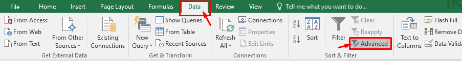
The Advanced Filter dialog box appears.
Specify the List range: i.e select the cells you need to apply the filter to. You can enter them manually, or click on the Collapse button ![]() , select the area and click Expand .
, select the area and click Expand .
First, select the Copy to another location. This copied the unique elements onto a new column.
Now, use the collapse and expand button to select the rows you want the unique elements to be copied.
Finally, check Unique records only. And click OK.
Thus the distinct elements are copied onto a new row.
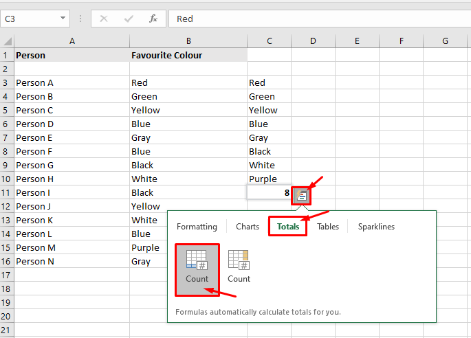
To calculate the row count, you can select the columns and click on Quick analysis or Ctrl + Q. Select Totals and click on Row Count. This will give you the row count right below the unique elements.
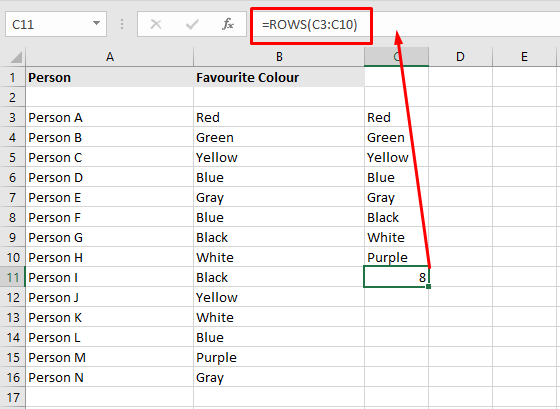
Or, you can use the function =ROWS(a:b), where a and b are the starting and ending cells respectively.
Note: If you click on Filter the list, in-place, the selected values will be replaced in the same column.
Using SUM and COUNTIF functions
You can use the SUM and COUNTIF functions to calculate the distinct values in Excel. In this case, we will inverse the COUNTIF function to arrive at distinct values.
To count distinct values in excel, first enter the formula =SUM(1/COUNTIF(range, range)) in the desired cell. The range specifies the starting cell and ending cell separated by a colon. This is an array function, so press Ctrl+Shift+Enter to apply the formula.

Alternatively, you can also use the formula =SUMPRODUCT(1/COUNTIF(range, range)) in the desired cell to count distinct values. This is not an array function, so pressing Enter is sufficient to apply the formula.
Consider the same above-mentioned example. To count the distinct values, enter the formula =SUM(1/COUNTIF(B3:B16, B3:B16)) in the destination cell. Here, the range is B3:B16, so the values in cells B3 to B16 are taken into account.
First, the COUNTIF function counts the number of times the values occur in the given range. This value is stored in an array. Then, this value is divided by 1. So, if a value occurs twice, the value after dividing by 1 will be 0.5. Now, the SUM or SUMPRODUCT function adds up the fractional values and returns the result which is equal to the count of distinct values in the range.
Note: Similarly, you can also tweak the formulae a little to find distinct text values or distinct numeric values.
To find distinct text values: =SUM(IF(ISTEXT(range),1/COUNTIF(range, range),””))
To find distinct text values: =SUM(IF(ISNUMBER(range),1/COUNTIF(range, range),””))
Closing Thoughts
Finding the unique and distinct elements in a large dataset can be used to determine the statistics or probability of the data.
In this guide, we saw how to count unique and distinct values in Excel. Based on your specifications and preferences, you can either find the count of unique or distinct values.
If you need more high-quality Excel guides, please check out our free Excel resources center.
Simon Sez IT has been teaching Excel for over ten years. For a low, monthly fee you can get access to 100+ IT training courses. Click here for advanced Excel courses with in-depth training modules.
Simon Calder

Chris “Simon” Calder was working as a Project Manager in IT for one of Los Angeles’ most prestigious cultural institutions, LACMA.He taught himself to use Microsoft Project from a giant textbook and hated every moment of it. Online learning was in its infancy then, but he spotted an opportunity and made an online MS Project course — the rest, as they say, is history!
Count unique values among duplicates
Excel for Microsoft 365 Excel for Microsoft 365 for Mac Excel for the web Excel 2021 Excel 2021 for Mac Excel 2019 Excel 2019 for Mac Excel 2016 Excel 2016 for Mac Excel 2013 Excel 2010 Excel 2007 Excel for Mac 2011 More…Less
Let’s say you want to find out how many unique values exist in a range that contains duplicate values. For example, if a column contains:
-
The values 5, 6, 7, and 6, the result is three unique values — 5 , 6 and 7.
-
The values «Bradley», «Doyle», «Doyle», «Doyle», the result is two unique values — «Bradley» and «Doyle».
There are several ways to count unique values among duplicates.
You can use the Advanced Filter dialog box to extract the unique values from a column of data and paste them to a new location. Then you can use the ROWS function to count the number of items in the new range.
-
Select the range of cells, or make sure the active cell is in a table.
Make sure the range of cells has a column heading.
-
On the Data tab, in the Sort & Filter group, click Advanced.
The Advanced Filter dialog box appears.
-
Click Copy to another location.
-
In the Copy to box, enter a cell reference.
Alternatively, click Collapse Dialog
 to temporarily hide the dialog box, select a cell on the worksheet, and then press Expand Dialog .
 -
Select the Unique records only check box, and click OK.
The unique values from the selected range are copied to the new location beginning with the cell you specified in the Copy to box.
-
In the blank cell below the last cell in the range, enter the ROWS function. Use the range of unique values that you just copied as the argument, excluding the column heading. For example, if the range of unique values is B2:B45, you enter =ROWS(B2:B45).
 to temporarily hide the dialog box, select a cell on the worksheet, and then press Expand Dialog
  .
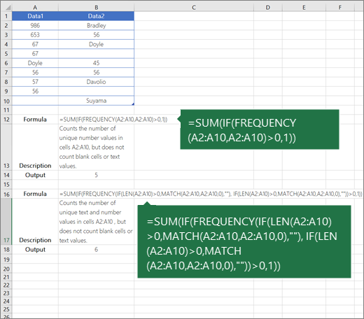
.Use a combination of the IF, SUM, FREQUENCY, MATCH, and LEN functions to do this task:
-
Assign a value of 1 to each true condition by using the IF function.
-
Add the total by using the SUM function.
-
Count the number of unique values by using the FREQUENCY function. The FREQUENCY function ignores text and zero values. For the first occurrence of a specific value, this function returns a number equal to the number of occurrences of that value. For each occurrence of that same value after the first, this function returns a zero.
-
Return the position of a text value in a range by using the MATCH function. This value returned is then used as an argument to the FREQUENCY function so that the corresponding text values can be evaluated.
-
Find blank cells by using the LEN function. Blank cells have a length of 0.
Notes:
-
The formulas in this example must be entered as array formulas. If you have a current version of Microsoft 365, then you can simply enter the formula in the top-left-cell of the output range, then press ENTER to confirm the formula as a dynamic array formula. Otherwise, the formula must be entered as a legacy array formula by first selecting the output range, entering the formula in the top-left-cell of the output range, and then pressing CTRL+SHIFT+ENTER to confirm it. Excel inserts curly brackets at the beginning and end of the formula for you. For more information on array formulas, see Guidelines and examples of array formulas.
-
To see a function evaluated step by step, select the cell containing the formula, and then on the Formulas tab, in the Formula Auditing group, click Evaluate Formula.
-
The FREQUENCY function calculates how often values occur within a range of values, and then returns a vertical array of numbers. For example, use FREQUENCY to count the number of test scores that fall within ranges of scores. Because this function returns an array, it must be entered as an array formula.
-
The MATCH function searches for a specified item in a range of cells, and then returns the relative position of that item in the range. For example, if the range A1:A3 contains the values 5, 25, and 38, the formula =MATCH(25,A1:A3,0) returns the number 2, because 25 is the second item in the range.
-
The LEN function returns the number of characters in a text string.
-
The SUM function adds all the numbers that you specify as arguments. Each argument can be a range, a cell reference, an array, a constant, a formula, or the result from another function. For example, SUM(A1:A5) adds all the numbers that are contained in cells A1 through A5.
-
The IF function returns one value if a condition you specify evaluates to TRUE, and another value if that condition evaluates to FALSE.
Need more help?
You can always ask an expert in the Excel Tech Community or get support in the Answers community.
See Also
Filter for unique values or remove duplicate values
Need more help?
Want more options?
Explore subscription benefits, browse training courses, learn how to secure your device, and more.
Communities help you ask and answer questions, give feedback, and hear from experts with rich knowledge.