
In this example, VLOOKUP is configured to look up 1000 invoice numbers in a table that contains 1 million invoices. Normally, this kind of lookup would perform quite slowly, because we would need to configure VLOOKUP to use an exact match, and exact match lookups on large data sets can be painfully slow. However, because the data is sorted by invoice number, we can use the modified VLOOKUP formula seen in the worksheet. Although this formula uses VLOOKUP twice, it performs well.
Exact-match VLOOKUP is slow
When you use VLOOKUP in «exact match mode» on a large set of data, it can really slow down the calculation time in a worksheet. With very large sets of data, the calculation time can be minutes. To use VLOOKUP in exact match mode, provide FALSE or zero as the fourth argument, range_lookup:
=VLOOKUP(value,data,n,FALSE) // exact match
The reason VLOOKUP is slow in this mode is that there is no requirement that the lookup values be sorted. As a result, VLOOKUP must check every record in the data set until a match is found, or not. This is sometimes referred to as a linear search.
Approximate-match VLOOKUP is very fast
In approximate-match mode, VLOOKUP is extremely fast. To use approximate-match VLOOKUP, sort the data by the first column (the lookup column), then specify TRUE for range_lookup or omit the argument:
=VLOOKUP(value,data,n,TRUE) // approximate match
=VLOOKUP(value,data,n) // approximate match
With very large sets of data, changing to approximate-match VLOOKUP can mean a dramatic speed increase. This is because VLOOKUP will assume data is sorted and use a different algorithm to speed up searching, sometimes called a binary search.
For a complete VLOOKUP overview with many examples, see How to use VLOOKUP.
The problem
At first glance, a solution seems simple: sort the data, and use VLOOKUP in approximate match mode. However, the problem is that VLOOKUP won’t return an error if a value is not found. Instead, it may return an incorrect result that looks completely normal. For example, in the worksheet shown, if we configure VLOOKUP to find the Amount for invoice 500010 with range_lookup set to TRUE, the result is 9225 even though invoice 500010 does not exist in the table:
=VLOOKUP(500010,data,2,TRUE) // returns 9225This happens because VLOOKUP’s behavior with approximate match enabled is «exact match or next smaller value». When VLOOKUP can’t find invoice 500010, it matches the next smaller invoice number, which is 500008, and returns 9225. So, while the formula runs very quickly, the result is not reliable. Obviously, this is not something you want to explain to your boss.
A solution with VLOOKUP + VLOOKUP
One way to speed up VLOOKUP in this situation is to use VLOOKUP twice, both times in approximate match mode. This may seem counterintuitive because we are calling VLOOKUP twice. However, two fast operations are better than one slow operation. The trick is to structure the formula in a way that leverages two fast lookups in a way that requires an exact match result. We do that by testing the result of the first VLOOKUP to see if did actually find the lookup value. In the worksheet shown, the formula in F5, copied down, is:
=IF(VLOOKUP(E5,data,1)=E5,VLOOKUP(E5,data,2),NA())Notice the IF function controls the flow of the formula. If we do find the lookup value, we run the second lookup. Otherwise, we return an error. The logical_test inside the IF function looks like this:
VLOOKUP(E5,data,1)=E5Here, we use VLOOKUP to find and return the lookup value itself, and we do so in approximate match mode by omitting the range_lookup argument. Remember, VLOOKUP defaults to an approximate match. Then we test the result against the lookup value. If this test returns TRUE, we know the lookup value exists in the data and we run the second VLOOKUP to fetch the desired value:
VLOOKUP(E5,data,2)However, if the test returns FALSE, it means we didn’t find the lookup value. In that case, we simply return an #N/A error with the NA function:
NA() // returns #N/ATo summarize: if we find the invoice number, we look up the amount. If we don’t find an invoice number return #N/A error, which tells us the invoice number does not exist in the data. Even though the formula uses the VLOOKUP function two times, performance is good, because both instances of VLOOKUP use approximate match mode, which runs very quickly.
Summary
With large sets of data, exact match VLOOKUP can run painfully slow when configured for an exact match. This is because there is no requirement that the lookup values be sorted and VLOOKUP must perform a linear search, which is a slow operation when there are many values to check. On the other hand, if data is sorted, VLOOKUP can be configured for an approximate match by setting range_lookup to TRUE, or by omitting range_lookup altogether. In this configuration, VLOOKUP runs very fast. However, VLOOKUP may return an incorrect result. This happens because VLOOKUP’s behavior with approximate match enabled is «exact match or next smaller value», so VLOOKUP matches the previous value when a match is not found. One way around this problem is to use VLOOKUP twice, both times in approximate match mode. The trick is to structure the formula in a way that leverages two fast lookups in a way that still ensures an exact match result.
Notes
- This approach is overkill unless lookup performance is an issue.
- Data must be sorted by lookup value in ascending order.
- The newer XLOOKUP function has a very fast binary search option.

4 different ways to perform LOOKUP with 2 lookup values
We know that VLOOKUP is very useful. At the same time, we know that VLOOKUP has its limitations. E.g. VLOOKUP only looks from left to right; VLOOKUP only handle one lookup value. For a simple situation shown below, VLOOKUP doesn’t seem to work (directly).
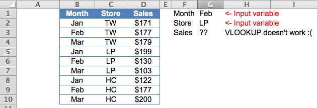
No worry. There are at least four workarounds!
- Using a helper column
- Using CHOOSE to recreate the Table Array for VLOOKUP
- Using INDEX, MATCH and = Operator
- Using SUMPRODUCT
Let’s start with the basic.
1. Using a helper column
Most of the time, complicated problem will become easier and manageable when it is broken down into small pieces. Same applies in formula building in Excel.
Take below example:
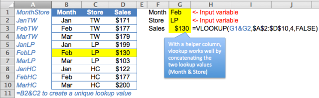
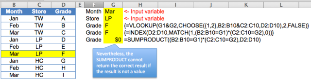
By CONCATENATING “Month” and “Store” in column A (note: better to put the helper column to the left of the original Table as VLOOKUP looks from left to right.), we create the lookup value required in column A. As a result, with the helper column A (which could be hidden later), the problem can be solved easily by
=VLOOKUP(G1&G2,$A$2:$D$10,4,FALSE)
Note: we need to combine the Month (G1) and Store (G2) as the lookup value
Non-helper column approach
Well, for any reason a helper column is not an option, we may do it by array formula. At least two different ways to perform the job:

2) Using CHOOSE to recreate the Table Array for VLOOKUP
This is a bit advance. The tricky part is to re-create the Table Array that is suitable for VLOOKUP by using CHOOSE.
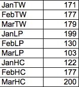
CHOOSE({1,2},B2:B10&C2:C10,D2:D10) does two things
- Combine “Month” and “Store” into a single array as “JanTW”;”FebTW”, etc……
- Join the two arrays into a “table” of two columns
When we evaluate the result of the above CHOOSE (by selecting the whole CHOOSE formula in the formula bar and then press F9, we get the following result:
{"JanTW",171;"FebTW",177;"MarTW",179;"JanLP",199;"FebLP",130;"MarLP",103;"JanHC",122;"FebHC",177;"MarHC",200}
To visualize it in a Table format, it looks like the below:
Now the whole formula makes sense:
=VLOOKUP(G1&G2,CHOOSE({1,2},B2:B10&C2:C10,D2:D10),2,FALSE)
 CTRL SHIFT ENTER (not just ENTER)
IMPORTANT: As this is an array formula, we have to input CTRL SHIFT ENTER to tell Excel that we are going to input array formula. You will see the {} in the formula bar if array formula is input successfully.
-
- Note: For both 1) and 2), the robust way to combine the lookup values should include a delimiter in between, e.g. A1 & “|” & B1 . Please read Pay attention when concatenate for explanation.
3) Using INDEX, MATCH and = Operator
=INDEX(D2:D10,MATCH(1,(B2:B10=G1)*(C2:C10=G2),0))
 CTRL SHIFT ENTER
This formula actually looks more intuitive. How?
First let’s understand what the (B2:B10=G1)*(C2:C10=G2) does?
- B2:B10=G1 asks Excel to evaluate if B2=G1, if yes, it returns TRUE; if no, it returns FALSE. Then do the same for B3=G1, B4=G1…… until B10=G1. An array of TRUE/FALSE will be the result.
- C2:C10=G2 basically does the same thing but look at different values.
When we compare the two array of TRUE/FALSE by multiplying them, only TRUE * TRUE gives the result of 1 (TRUE). A picture tells more. Let’s take a look at the screenshot below:
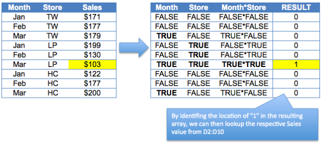
Bingo, we can identify the row that meets both lookup values.
Now you should be able to use MATCH to identify the position of the matching values. Then use INDEX to return the result required.
- =INDEX(D2:D10,MATCH(1,(B2:B10=G1)*(C2:C10=G2),0)) gives
- =INDEX(D2:D10,MATCH(1,{0;0;0;0;0;1;0;0;0},0) gives
- =INDEX(D2:D10,6) returns
- $103, the correct result!
4) Using SUMPRODUCT
SUMPRODUCT is a powerful function in Excel. I am going to write separate posts about SUMPRODUCT later. Although SUMPRODUCT seems to work in our example, it actually fails if the result we want is text instead of value.
To understand that, we have to understand how SUMPRODUCT behaves. If you want to know more about SUMPRODUCT, stay tuned! 🙂
So, which one do I use?
Although options 2) and 3) works fine, I prefer option 1) under normal circumstance. Why?
In daily work life, I believe it is more important to build a spreadsheet that is manageable and readable by most users (including myself)… Not every one in workplace is Excel guru. If every one is, we don’t have to spend so much time to fight with spreadsheets.
As such, let’s obey the KISS principle whenever possible.
Other topics about vlookup:
- The basic of vlookup
- Tips in constructing vlookup
- vlookup with Match
- vlookup options – True or False?
- Advanced vlookup – Text vs. Number
- Advanced vlookup – Wildcard Characters “?” and “*”
- Alternative to vlookup – Index and Match
- Three different ways to do case-sensitive lookup


About MF
An Excel nerd who just transition into a role related to data analytics at current company……😊
Recently in love with Power Query and Power BI.😍
Keep learning new Excel and Power BI stuffs and be amazed by all the new discoveries.
Excel for Microsoft 365 Excel for Microsoft 365 for Mac Excel for the web Excel 2021 Excel 2021 for Mac Excel 2019 Excel 2019 for Mac Excel 2016 Excel 2016 for Mac Excel 2013 Excel 2010 Excel 2007 Excel for Mac 2011 Excel Starter 2010 More…Less
Tip: Try using the new XLOOKUP function, an improved version of VLOOKUP that works in any direction and returns exact matches by default, making it easier and more convenient to use than its predecessor.
Use VLOOKUP when you need to find things in a table or a range by row. For example, look up a price of an automotive part by the part number, or find an employee name based on their employee ID.
In its simplest form, the VLOOKUP function says:
=VLOOKUP(What you want to look up, where you want to look for it, the column number in the range containing the value to return, return an Approximate or Exact match – indicated as 1/TRUE, or 0/FALSE).

Tip: The secret to VLOOKUP is to organize your data so that the value you look up (Fruit) is to the left of the return value (Amount) you want to find.
Use the VLOOKUP function to look up a value in a table.
Syntax
VLOOKUP (lookup_value, table_array, col_index_num, [range_lookup])
For example:
-
=VLOOKUP(A2,A10:C20,2,TRUE)
-
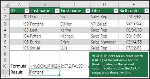
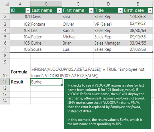
=VLOOKUP(«Fontana»,B2:E7,2,FALSE)
-
=VLOOKUP(A2,’Client Details’!A:F,3,FALSE)
|
Argument name |
Description |
|---|---|
|
lookup_value (required) |
The value you want to look up. The value you want to look up must be in the first column of the range of cells you specify in the table_array argument. For example, if table-array spans cells B2:D7, then your lookup_value must be in column B.
|
|
table_array (required) |
The range of cells in which the VLOOKUP will search for the lookup_value and the return value. You can use a named range or a table, and you can use names in the argument instead of cell references. The first column in the cell range must contain the lookup_value. The cell range also needs to include the return value you want to find. Learn how to select ranges in a worksheet. |
|
col_index_num (required) |
The column number (starting with 1 for the left-most column of table_array) that contains the return value. |
|
range_lookup (optional) |
A logical value that specifies whether you want VLOOKUP to find an approximate or an exact match:
|
How to get started
There are four pieces of information that you will need in order to build the VLOOKUP syntax:
-
The value you want to look up, also called the lookup value.
-
The range where the lookup value is located. Remember that the lookup value should always be in the first column in the range for VLOOKUP to work correctly. For example, if your lookup value is in cell C2 then your range should start with C.
-
The column number in the range that contains the return value. For example, if you specify B2:D11 as the range, you should count B as the first column, C as the second, and so on.
-
Optionally, you can specify TRUE if you want an approximate match or FALSE if you want an exact match of the return value. If you don’t specify anything, the default value will always be TRUE or approximate match.
Now put all of the above together as follows:
=VLOOKUP(lookup value, range containing the lookup value, the column number in the range containing the return value, Approximate match (TRUE) or Exact match (FALSE)).
Examples
Here are a few examples of VLOOKUP:
Example 1

Example 2
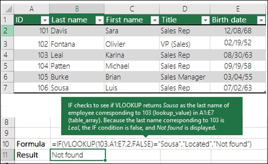
Example 3
Example 4
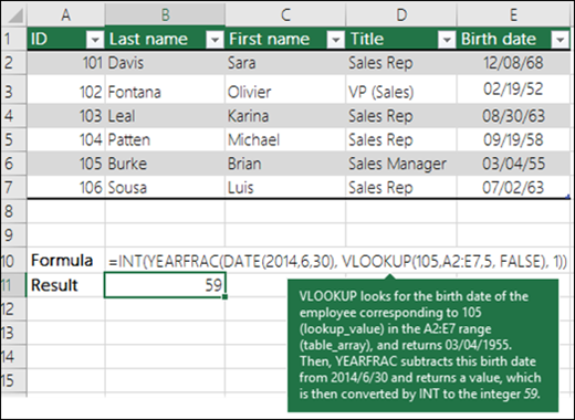
Example 5
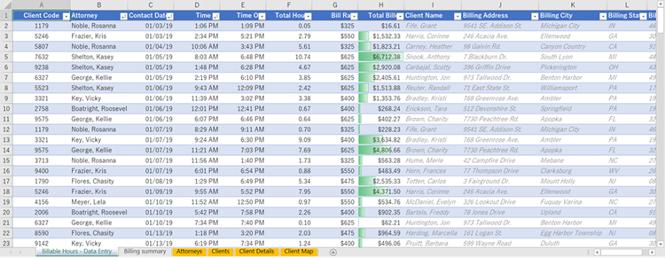
You can use VLOOKUP to combine multiple tables into one, as long as one of the tables has fields in common with all the others. This can be especially useful if you need to share a workbook with people who have older versions of Excel that don’t support data features with multiple tables as data sources — by combining the sources into one table and changing the data feature’s data source to the new table, the data feature can be used in older Excel versions (provided the data feature itself is supported by the older version).
|
|
Here, columns A-F and H have values or formulas that only use values on the worksheet, and the rest of the columns use VLOOKUP and the values of column A (Client Code) and column B (Attorney) to get data from other tables. |
-
Copy the table that has the common fields onto a new worksheet, and give it a name.
-
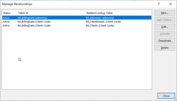
Click Data > Data Tools > Relationships to open the Manage Relationships dialog box.

-
For each listed relationship, note the following:
-
The field that links the tables (listed in parentheses in the dialog box). This is the lookup_value for your VLOOKUP formula.
-
The Related Lookup Table name. This is the table_array in your VLOOKUP formula.
-
The field (column) in the Related Lookup Table that has the data you want in your new column. This information is not shown in the Manage Relationships dialog — you’ll have to look at the Related Lookup Table to see which field you want to retrieve. You want to note the column number (A=1) — this is the col_index_num in your formula.
-
-
To add a field to the new table, enter your VLOOKUP formula in the first empty column using the information you gathered in step 3.
In our example, column G uses Attorney (the lookup_value) to get the Bill Rate data from the fourth column (col_index_num = 4) from the Attorneys worksheet table, tblAttorneys (the table_array), with the formula =VLOOKUP([@Attorney],tbl_Attorneys,4,FALSE).
The formula could also use a cell reference and a range reference. In our example, it would be =VLOOKUP(A2,’Attorneys’!A:D,4,FALSE).
-
Continue adding fields until you have all the fields that you need. If you are trying to prepare a workbook containing data features that use multiple tables, change the data source of the data feature to the new table.
|
Problem |
What went wrong |
|---|---|
|
Wrong value returned |
If range_lookup is TRUE or left out, the first column needs to be sorted alphabetically or numerically. If the first column isn’t sorted, the return value might be something you don’t expect. Either sort the first column, or use FALSE for an exact match. |
|
#N/A in cell |
For more information on resolving #N/A errors in VLOOKUP, see How to correct a #N/A error in the VLOOKUP function. |
|
#REF! in cell |
If col_index_num is greater than the number of columns in table-array, you’ll get the #REF! error value. For more information on resolving #REF! errors in VLOOKUP, see How to correct a #REF! error. |
|
#VALUE! in cell |
If the table_array is less than 1, you’ll get the #VALUE! error value. For more information on resolving #VALUE! errors in VLOOKUP, see How to correct a #VALUE! error in the VLOOKUP function. |
|
#NAME? in cell |
The #NAME? error value usually means that the formula is missing quotes. To look up a person’s name, make sure you use quotes around the name in the formula. For example, enter the name as «Fontana» in =VLOOKUP(«Fontana»,B2:E7,2,FALSE). For more information, see How to correct a #NAME! error. |
|
#SPILL! in cell |
This particular #SPILL! error usually means that your formula is relying on implicit intersection for the lookup value, and using an entire column as a reference. For example, =VLOOKUP(A:A,A:C,2,FALSE). You can resolve the issue by anchoring the lookup reference with the @ operator like this: =VLOOKUP(@A:A,A:C,2,FALSE). Alternatively, you can use the traditional VLOOKUP method and refer to a single cell instead of an entire column: =VLOOKUP(A2,A:C,2,FALSE). |
|
Do this |
Why |
|---|---|
|
Use absolute references for range_lookup |
Using absolute references allows you to fill-down a formula so that it always looks at the same exact lookup range. Learn how to use absolute cell references. |
|
Don’t store number or date values as text. |
When searching number or date values, be sure the data in the first column of table_array isn’t stored as text values. Otherwise, VLOOKUP might return an incorrect or unexpected value. |
|
Sort the first column |
Sort the first column of the table_array before using VLOOKUP when range_lookup is TRUE. |
|
Use wildcard characters |
If range_lookup is FALSE and lookup_value is text, you can use the wildcard characters—the question mark (?) and asterisk (*)—in lookup_value. A question mark matches any single character. An asterisk matches any sequence of characters. If you want to find an actual question mark or asterisk, type a tilde (~) in front of the character. For example, =VLOOKUP(«Fontan?»,B2:E7,2,FALSE) will search for all instances of Fontana with a last letter that could vary. |
|
Make sure your data doesn’t contain erroneous characters. |
When searching text values in the first column, make sure the data in the first column doesn’t have leading spaces, trailing spaces, inconsistent use of straight ( ‘ or » ) and curly ( ‘ or “) quotation marks, or nonprinting characters. In these cases, VLOOKUP might return an unexpected value. To get accurate results, try using the CLEAN function or the TRIM function to remove trailing spaces after table values in a cell. |
Need more help?
You can always ask an expert in the Excel Tech Community or get support in the Answers community.

See Also
XLOOKUP function
Video: When and how to use VLOOKUP
Quick Reference Card: VLOOKUP refresher
How to correct a #N/A error in the VLOOKUP function
Look up values with VLOOKUP, INDEX, or MATCH
HLOOKUP function
Need more help?
Want more options?
Explore subscription benefits, browse training courses, learn how to secure your device, and more.
Communities help you ask and answer questions, give feedback, and hear from experts with rich knowledge.
Watch Video – How to Use VLOOKUP Function with Multiple Criteria
Excel VLOOKUP function, in its basic form, can look for one lookup value and return the corresponding value from the specified row.
But often there is a need to use the Excel VLOOKUP with multiple criteria.
How to Use VLOOKUP with Multiple Criteria
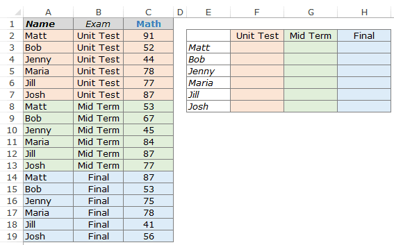
Suppose you have a data with students name, exam type, and the Math score (as shown below):
Using the VLOOKUP function to get the Math score for each student for respective exam levels could be a challenge.
One can argue that a better option would be to restructure the data set or use a Pivot Table. If that works for you, nothing like that. But in many cases, you are stuck with the data that you have and pivot table may not be an option.
In such cases, this tutorial is for you.
Now there are two ways you can get the lookup value using VLOOKUP with multiple criteria.
- Using a Helper Column.
- Using the CHOOSE function.
VLOOKUP with Multiple Criteria – Using a Helper Column
I am a fan of helper columns in Excel.
I find two significant advantages of using helper columns over array formulas:
- It makes it easy to understand what’s going on in the worksheet.
- It makes it faster as compared with the array functions (noticeable in large data sets).
Now, don’t get me wrong. I am not against array formulas. I love the amazing things can be done with array formulas. It’s just that I save them for special occasions when all other options are of no help.
Coming back to the question in point, the helper column is needed to create a unique qualifier. This unique qualifier can then be used to lookup the correct value. For example, there are three Matt in the data, but there is only one combination of Matt and Unit Test or Matt and Mid-Term.
Here are the steps:
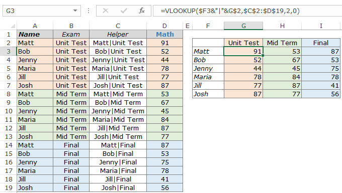
How does this work?
We create unique qualifiers for each instance of a name and the exam. In the VLOOKUP function used here, the lookup value was modified to $F3&”|”&G$2 so that both the lookup criteria are combined and are used as a single lookup value. For example, the lookup value for the VLOOKUP function in G2 is Matt|Unit Test. Now this lookup value is used to get the score from C2:D19.
Clarifications:
There are a couple of questions that are likely to come to your mind, so I thought I will try and answer it here:
- Why have I used | symbol while joining the two criteria? – In some exceptionally rare (but possible) conditions, you may have two criteria that are different but ends up giving the same result when combined. Here is a very simple example (forgive me for my lack of creativity here):
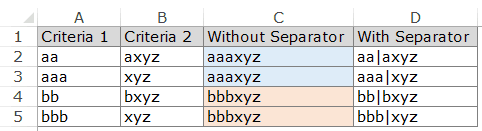
Note that while A2 and A3 are different and B2 and B3 are different, the combinations end up being the same. But if you use a separator, then even the combination would be different (D2 and D3).
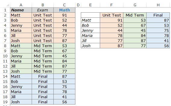
- Why did I insert the helper column between column B and C and not in the extreme left? – There is no harm in inserting the helper column to the extreme left. In fact, if you don’t want to temper with the original data, that should be the way to go. I did it as it makes me use less number of cells in the VLOOKUP function. Instead of having 4 columns in the table array, I could manage with only 2 columns. But that’s just me.
Now there is no one size that fits all. Some people may prefer to not use any helper column while using VLOOKUP with multiple criteria.
So here is the non-helper column method for you.
Download the Example File

VLOOKUP with Multiple Criteria – Using the CHOOSE Function
Using array formulas instead of helper columns saves you worksheet real estate, and the performance can be equally good if used less number of times in a workbook.
Considering the same data set as used above, here is the formula that will give you the result:
=VLOOKUP($E3&”|”&F$2,CHOOSE({1,2},$A$2:$A$19&”|”&$B$2:$B$19,$C$2:$C$19),2,0)
Since this is an array formula, use it with Control + Shift + Enter, instead of just Enter.
How does this work?
The formula also uses the concept of a helper column. The difference is that instead of putting the helper column in the worksheet, consider it as virtual helper data that is a part of the formula.
Let me show you what I mean by virtual helper data.
In the above illustration, as I select the CHOOSE part of the formula and press F9, it shows the result that the CHOOSE formula would give.
The result is {“Matt|Unit Test”,91;”Bob|Unit Test”, 52;……}
It’s an array where a comma represents next cell in the same row and semicolon represents that the following data is in the next column. Hence, this formula creates 2 columns of data – One column has the unique identifier and one has the score.
Now, when you use the VLOOKUP function, it simply looks for the value in the first column (of this virtual 2 column data) and returns the corresponding score.
Download the Example File
You can also use other formulas to do a lookup with multiple criteria (such as INDEX/MATCH or SUMPRODUCT).
Is there any other way you know to do this? If yes, do share with me in the comments section.
You May Also Like the Following LOOKUP Tutorials:
- VLOOKUP Vs. INDEX/MATCH
- Get Multiple Lookup Values Without Repetition in a Single Cell.
- How to make VLOOKUP Case Sensitive.
- Use IFERROR with VLOOKUP to Get Rid of #N/A Errors.
Skip to content
Очень часто наши требования к поиску данных не ограничиваются одним условием. К примеру, нам нужна выручка по магазину за определенный месяц, количество конкретного товара, проданного определенному покупателю и т.д. Обычными средствами функции ВПР эту задачу решить сложно и даже не всегда возможно. Ведь там предусмотрено использование только одного критерия поиска.
Мы предложим вам несколько вариантов решения проблемы поиска по нескольким условиям.
- ВПР по нескольким условиям с использованием дополнительного столбца.
- ВПР по двум условиям при помощи формулы массива.
- ВПР по нескольким критериям с применением массивов — способ 2.
- Двойной ВПР при помощи ИНДЕКС + ПОИСКПОЗ
- Достойная замена – функция СУММПРОИЗВ.
ВПР по нескольким условиям с использованием дополнительного столбца.
Задачу, рассмотренную в предыдущем примере, можно решить и другим способом – без использования формулы массива. Ведь работа с массивами многим представляется сложной и недоступной для понимания. Дополнительный столбец для поиска по нескольким условиям будет в определенном отношении более простым вариантом.
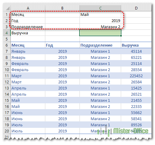
Итак, необходимо выбрать значение выручки за определенный месяц, год и по нужному магазину. В итоге имеем 3 условия отбора.
Сразу по трем столбцам функция ВПР искать не может. Поэтому нам нужно объединить их в один. И, поскольку поиск производится всегда в крайнем левом (первом) столбце, то нужно добавить его в нашу таблицу тоже слева.
Вставляем перед таблицей с данными дополнительный столбец A. Затем при помощи оператора & объединяем в нем содержимое B,C и D. Записываем в А7
=B7&C7&D7
и копируем в находящиеся ниже ячейки.
Формула поиска в D4 будет выглядеть:
=ВПР(D1&D2&D3;A7:E20;5;0)
В диапазон поиска включаем и наш дополнительный столбец. Критерий поиска – также объединение 3 значений. И извлекаем результат из 5 колонки.
Все работает, однако вид несколько портит дополнительный столбец. В крайнем случае, его можно скрыть, используя контекстное меню по нажатию правой кнопки мыши.

Вид станет приятнее, а на результаты это никак не повлияет.
ВПР по двум условиям при помощи формулы массива.
У нас есть таблица, в которой записана выручка по каждому магазину за день. Мы хотим быстро найти сумму продаж по конкретному магазину за определенный день.
Для этого в верхней части нашего листа запишем критерии поиска: дата и магазин. В ячейке B3 будем выводить сумму выручки.
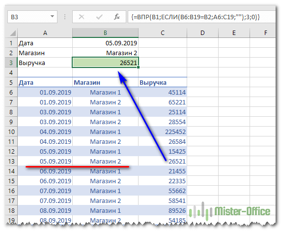
Формула в B3 выглядит следующим образом:
{=ВПР(B1;ЕСЛИ(B6:B19=B2;A6:C19;»»);3;0)}
Обратите внимание на фигурные скобки, которые означают, что это формула массива. То есть наша функция ВПР работает не с отдельными значениями, а разу с массивами данных.
Разберем процесс подробно.
Мы ищем дату, записанную в ячейке B1. Но вот только разыскивать мы ее будем не в нашем исходном диапазоне данных, а в немного видоизмененном. Для этого используем условие
ЕСЛИ(B6:B19=B2;A6:C19;»»)
То есть, в том случае, если наименование магазина совпадает с критерием в ячейке B2, мы оставляем исходные значения из нашего диапазона. А если нет – заменяем их на пробелы. И так по каждой строке.
В результате получим вот такой виртуальный массив данных на основе нашей исходной таблицы:

Как видите, строки, в которых ранее был «Магазин 1», заменены на пустые. И теперь искать нужную дату мы будем только среди информации по «Магазин 2». И извлекать значения выручки из третьей колонки.
С такой работой функция ВПР вполне справится.
Такой ход стал возможен путем применения формулы массива. Поэтому обратите особое внимание: круглые скобки в формуле писать руками не нужно! В ячейке B3 вы записываете формулу
=ВПР(B1;ЕСЛИ(B6:B19=B2;A6:C19;»»);3;0)
И затем нажимаете комбинацию клавиш CTRL+Shift+Enter. При этом Excel поймет, что вы хотите ввести формулу массива и сам подставит скобки.
Таким образом, функция ВПР поиск по двум столбцам производит в 2 этапа: сначала мы очищаем диапазон данных от строк, не соответствующих одному из условий, при помощи функции ЕСЛИ и формулы массива. А затем уже в этой откорректированной информации производим обычный поиск по одному только второму критерию при помощи ВПР.
Чтобы упростить работу в будущем и застраховать себя от возможных ошибок при добавлении новой информации о продажах, мы рекомендуем использовать «умную» таблицу. Она автоматически подстроит свой размер с учетом добавленных строк, и никакие ссылки в формулах не нужно будет менять.

Вот как это будет выглядеть.
ВПР по нескольким критериям с применением массивов — способ 2.
Выше мы уже рассматривали, как при помощи формулы массива можно организовать поиск ВПР с несколькими условиями. Предлагаем еще один способ.
Условия возьмем те же, что и в предыдущем примере.
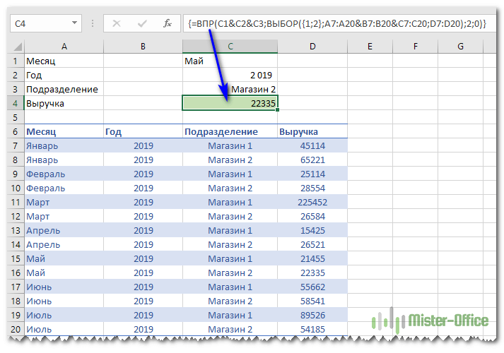
Формулу в С4 введем такую:
=ВПР(C1&C2&C3;ВЫБОР({1;2};A7:A20&B7:B20&C7:C20;D7:D20);2;0)
Естественно, не забываем нажать CTRL+Shift+Enter.
Теперь давайте пошагово разберем, как это работает.
Наше задача здесь – также создать дополнительный столбец для работы функции ВПР. Только теперь мы создаем его не на листе рабочей книги Excel, а виртуально.
Как и в предыдущем примере, мы ищем текст из объединенных в одно целое условий поиска.
Далее определяем данные, среди которых будем искать.
ВЫБОР({1;2};A7:A20&B7:B20&C7:C20;D7:D20)
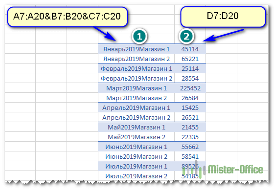
Конструкция вида A7:A20&B7:B20&C7:C20;D7:D20 создает 2 элемента. Первый – это объединение колонок A, B и C из исходных данных. Если помните, то же самое мы делали в нашем дополнительном столбце. Второй D7:D20 – это значения, одно из которых нужно в итоге выбрать.
Функция ВЫБОР позволяет из этих элементов создать массив. {1,2} как раз и означает, что нужно взять сначала первый элемент, затем второй, и объединить их в виртуальную таблицу – массив.
В первой колонке этой виртуальной таблицы мы будем искать, а из второй – извлекать результат.
Таким образом, для работы функции ВПР с несколькими условиями мы вновь используем дополнительный столбец. Только создаем его не реально, а виртуально.
Двойной ВПР при помощи ИНДЕКС + ПОИСКПОЗ
Далее речь у нас пойдет уже не о функции ВПР, но задачу мы будем решать ту же самую. В качестве критерия поиска нам опять нужно использовать несколько условий.
Существуют, пожалуй, даже более гибкие решения, нежели функция ВПР. Это комбинация функций ИНДЕКС + ПОИСКПОЗ.
Область их применения очень велика, о чем бы также будем рассказывать на сайте mister-office.ru.
А пока вернемся вновь к нашей задаче.

Формула в С4 теперь выглядит так:
=ИНДЕКС(D7:D20;ПОИСКПОЗ(1;(A7:A20=C1)*(B7:B20=C2)*(C7:C20=C3);0))
И не забываем при вводе нажать CTRL+Shift+Enter! Это формула массива.
Теперь давайте разбираться, как это работает.
Функция ИНДЕКС в нашем случае позволяет извлечь элемент из списка по его порядковому номеру. Список – это диапазон D7:D20, где записаны суммы выручки. А вот порядковый номер, который нужно извлечь, мы определяем при помощи ПОИСКПОЗ.
Синтаксис здесь следующий:
ПОИСКПОЗ(что_ищем; где_ищем; тип_поиска)
Тип поиска ставим 0, то есть точное совпадение. В нашем случае мы будем искать 1. Далее мы определим массив, в котором будем работать.
Выражение (A7:A20=C1)*(B7:B20=C2)*(C7:C20=C3) позволит создать виртуальную таблицу примерно такого вида:

Как видите, первоначально мы последовательно сравниваем каждое значение с нашим критерием отбора. В столбце А у нас записаны месяцы – сравниваем их с месяцем-критерием из ячейки C1. В случае совпадения получаем ИСТИНА, иначе – ЛОЖЬ. Аналогично последовательно проверяем год и название магазина. А затем просто перемножаем значения. Поскольку логические переменные для Excel – это либо 0, либо 1, то произведение их может быть равно 1 только в том случае, если мы имеем по каждой колонке ИСТИНА (то есть,1). Во всех остальных случаях получаем 0.
Убеждаемся, что цифра 1 встречается только единожды.
При помощи ПОИСКПОЗ определяем, на какой позиции она находится. На какой позиции находится 1, на той же позиции находится в массиве и искомая сумма выручки. В нашем случае это 10-я.
Далее при помощи ИНДЕКС извлекаем 10-ю по счету выручку.

Таким образом мы выбрали значение по нескольким условиям без использования функции ВПР.
Достойная замена – функция СУММПРОИЗВ.
У нас есть данные о продажах нескольких менеджеров в различных регионах. Нужно сделать выборку по дате, менеджеру и региону.
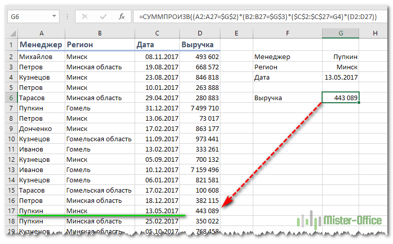
Поясним расчеты.
Выражение
=СУММПРОИЗВ((A2:A27=$G$2)*(B2:B27=$G$3)*($C$2:$C$27=G4)*(D2:D27))
Работает как формула массива, хотя по факту таковой не является. В этом заключается замечательное свойство функции СУММПРОИЗВ, о которой мы еще много будем говорить в других статьях.
Последовательно по каждой строке диапазона от 2-й до 27-й она проверяет совпадение каждого соответствующего значения с критерием поиска. Эти результаты перемножаются между собой и в итоге еще умножаются на сумму выручки. Если среди трех условий будет хотя бы одно несовпадение, то итогом будет 0. В случае совпадения сумма выручки трижды умножится на 1.
Затем все эти 27 произведений складываются, и результатом будет выручка нужного менеджера в каком-то регионе за определенную дату.
В качестве бонуса можно продолжить этот пример и рассчитать общую сумму продаж менеджера в определенном регионе.

Для этого из формулы просто уберем сравнение по дате.
=СУММПРОИЗВ((A2:A27=$G$2)*(B2:B27=$G$3)*(D2:D27))
Кстати, возможен и другой вариант расчета с этой же функцией:
=СУММПРОИЗВ(—(A2:A27=$G$2);—(B2:B27=$G$3);(D2:D27))
Итак, мы рассмотрели примеры использования функции ВПР с двумя и с несколькими условиями. А также обнаружили, что этой ценной функции есть замечательная альтернатива.
[the_ad_group id=»48″]
Примеры использования функции ВПР: