
Excel for Microsoft 365 Excel for Microsoft 365 for Mac Excel for the web Excel 2021 Excel 2021 for Mac Excel 2019 Excel 2019 for Mac Excel 2016 Excel 2016 for Mac Excel 2013 More…Less
This article describes the formula syntax and usage of the SHEETS
function in Microsoft Excel.
Description
Returns the number of sheets in a reference.
Syntax
SHEETS(reference)
The SHEETS function syntax has the following arguments.
-
Reference Optional. Reference is a reference for which you want to know the number of sheets it contains. If Reference is omitted, SHEETS returns the number of sheets in the workbook that contains the function.
Remarks
-
SHEETS includes all worksheets (visible, hidden, or very hidden) in addition to all other sheet types (macro, chart, or dialog sheets).
-
If reference is not a valid value, SHEETS returns the #REF! error value.
-
SHEETS is not available in the Object Model (OM) because the Object Model already includes similar functionality.
Example
Copy the example data in the following table, and paste it in cell A1 of a new Excel worksheet. For formulas to show results, select them, press F2, and then press Enter. If you need to, you can adjust the column widths to see all the data.
|
Formula |
Description |
Result |
|
=SHEETS() |
Because there is no Reference argument specified, the total number of sheets in the workbook is returned (3). |
3 |
|
=SHEETS(My3DRef) |
Returns the number of sheets in a 3D reference with the defined name My3DRef, which includes Sheet2 and Sheet3 (2). |
2 |
Top of Page
Need more help?
Want more options?
Explore subscription benefits, browse training courses, learn how to secure your device, and more.
Communities help you ask and answer questions, give feedback, and hear from experts with rich knowledge.
Содержание
- Examples of using the SHEET and SHEETS functions in Excel formulas
- SHEET and SHEETS functions in Excel: description of arguments and syntax
- How to get sheet name by formula in Excel
- Examples of using the SHEET function and SHEETS
- Processing information about the sheets of the book on the formula Excel
- Function SHEETS and formulas for working with other sheets in Excel
- Formulas using links to other Excel sheets
- SHEETS function to count the number of sheets in a workbook
- Links to other sheets in document templates
- How can I get a list of all the sheets that are in a file on one sheet?
- 6 Answers 6
- Excel formula apply conditions to all sheets same whole column
Examples of using the SHEET and SHEETS functions in Excel formulas
SHEET function in Excel returns a numeric value corresponding to the sheet number referenced by the link passed to the function as a parameter.
SHEET and SHEETS functions in Excel: description of arguments and syntax
SHEETS function in Excel returns a numeric value that corresponds to the number of sheets referenced.
- Both functions are useful for use in documents containing a large number of sheets.
- A sheet in Excel is a table of all the cells that are displayed on the screen and are outside of it (a total of 1,048,576 rows and 16,384 columns). When sending a sheet to print, it can be divided into several pages. Therefore, the terms “sheet” and “page” should not be confused.
- The number of sheets in the book is limited only by the amount of PC RAM.
Function has only 1 argument in its syntax and is optional for: =SHEET( value ).
- value is an optional function argument that contains text data with the name of the sheet or a link for which you want to set the sheet number. If this parameter is not specified, the function will return the number of the sheet in one of the cells of which it was written.
- When the sheet works, all sheets that are visible, hidden and very hidden are taken into account. Exceptions are dialogs, macros, and diagrams.
- If the function argument is a text value that does not match the name of any of the sheets contained in the book, the error #NA will be returned.
- If an invalid value was passed as an argument to the function, the result of its calculation will be the error #REF!.
- Within the object model (the hierarchy of objects in VBA, in which Application is the main object and Workbook, WorkSheet, etc., are child objects), the SHEET function is not available because it contains a similar function.
The function has the following syntax: =SHEETS( reference ).
- reference — an object of reference type for which you want to determine the number of sheets. This argument is optional. If this parameter is not specified, the function will return the number of sheets contained in the book where it was written.
- This function counts the number of all hidden, very hidden and visible sheets, with the exception of charts, macros and dialogs.
- If an invalid reference was passed as a parameter, the result of the calculation is the error code #REF!.
- This function is not available in the object model due to the presence of a similar function there.
How to get sheet name by formula in Excel
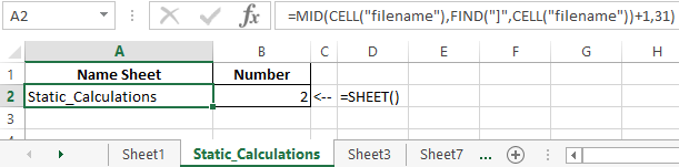
Example 1. In carrying out the calculated work the student used the Excel program, in which he created a book of several sheets. For his own convenience, the student decided to display in the cells A2 and B2 of each sheet data on the name of the sheet and its serial number, respectively. For this, he used the following formulas:
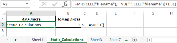
Description of arguments for the MID function:
- =CELL(«filename») is a function that returns text in which the MID function searches for a specified number of characters. In this case, the value “C:UserssoulpDesktop[Workbook.xlsx] Static_Calculations” will return, where after the “]” symbol is the required text — the name.
- =FIND(«]»,CELL(«filename»))+1 is a function that returns the position number of the character «]», one is added so that the MID function does not take into account the character].
- 31 — the maximum number of characters in the name.
=SHEET() — this function without parameter returns the number of the current sheet. As a result of its calculation, we get the number of sheets in the current book.
Examples of using the SHEET function and SHEETS
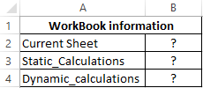
Example 2. The Excel workbook contains several sheets. It is necessary:
- Return the current sheet number.
- Return the sheet number with the name «Static_calculations».
- Return the number of the sheet «Dynamic_calculations», if its cell A3 contains the value 0.
Enter the data in the table:
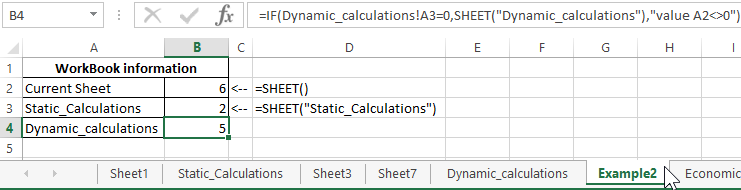
Next, we write the formulas for all 4 conditions:
- For condition # 1, use the following formula: =SHEET()
- For condition # 2, enter the formula: =SHEET(«Static_calculations»)
- For condition number 3 we write the formula:
0″)’ >
The IF function checks whether the value stored in the A3 cell of the Dynamic_ calculations is equal to zero or null.
As a result, we get:
Processing information about the sheets of the book on the formula Excel
Example 3. To determine the contains several sheets. It is necessary to determine the total number of sheets, as well as the number contained between the “Static_calculations” and “Economic_calculations”.
The source table is:
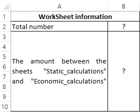
The total number of sheets is calculated by the formula:
To determine the number contained between these two sheets, we write the formula:
- Static_calculations: Economic_calculations!A2 — A reference to cell A2 of the range of sheets between «Static_calculations» and «Economic_calculations» including these sheets.
- To get the desired value, 2 was subtracted.
As a result, we get the following:
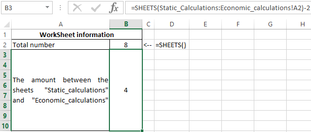
The formula displays detailed information on the data on the sheets in a certain range of their location in the Excel workbook.
Источник
Function SHEETS and formulas for working with other sheets in Excel
SHEET function is designed to return the number of a specific sheet with a space, which allows access to the entire workbook in MS Excel. SHEETS function provides the user with information on the number of sheets contained in the workbook.
Formulas using links to other Excel sheets
Suppose we have a company DecArt in which employees work and their monthly, salary is calculated. This company has information about the average monthly salary in Excel, and the data on it are placed on different sheets: on sheet 1 there are data on wages, on sheet 2, the percentage bonus. We need to calculate the size of the premium in dollars, while these data were placed on the second sheet.
To begin, consider an example of working with sheets in Excel formulas. Example 1:
- Let’s create on sheet 1 of the workbook of the spreadsheet Excel processor table, as shown in the figure. Information about the average monthly wage:

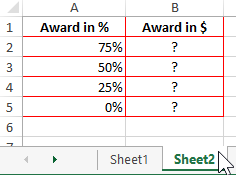
- Next, on sheet 2 of the workbook, we will prepare an area for placing our result — the size of our premium in dollars, as shown in the figure:
- Next, we will need to enter into the B2 cell the formula shown in the figure below:
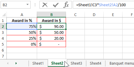
This formula was entered as follows: first, in cell B2, we set the «=» sign, then clicked on «Sheet1» in the lower left corner of the workbook and went to cell C3 on sheet 1, then entered the multiplication operation and switched again to «Sheet2 «to add a percentage.
Thus, when calculating the bonus of each employee, we obtained the initial data on one sheet, and the calculation was made on another sheet. This formula will be very useful when working with longer data sets in large organizations.
SHEETS function to count the number of sheets in a workbook
Consider now the example of the function. It often happens that there are too many sheets in an Excel workbook. It is not possible to visually find out their exact number; it is for this purpose that the SHEETS function has been created.
In this function, only 1 argument — «Link» and even then optional. If it is not filled, then the function returns the total number of sheets created in the current workbook of the Excel file. If necessary, you can fill in the argument. To do this, it is necessary to specify a link to the workbook, in which you need to calculate the total number of sheets created in it.
Example 2. Suppose we have a firm for the production of upholstered furniture, and it has a lot of documents that are contained in the Excel workbook. We need to calculate the exact number of these documents, since each of them has its own name, then it will take time to visually calculate their number.
The figure below shows the approximate number:
To organize the counting of all sheets, you must use function. Simply set the equal sign “=” and enter the function without filling its arguments in brackets. The call to this function is shown below:
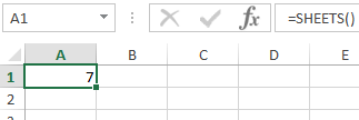
As a result, we obtain the following value: 12 sheets.
Thus, we learned that our company has 12 documents contained in an Excel workbook. This simple example clearly illustrates the operation of the function. This feature can be useful for managers, office workers, sales managers.
Links to other sheets in document templates
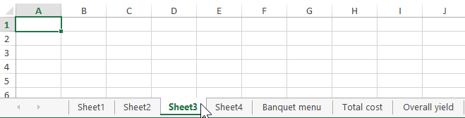
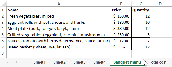
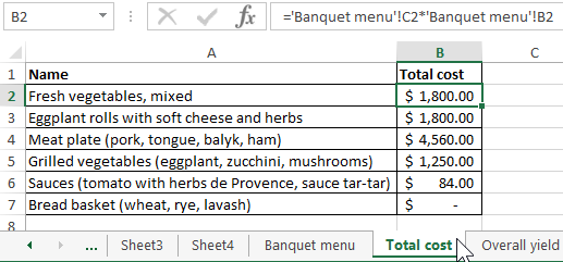
Example 3. There are data on the cost of a banquet company engaged in on-site service. It is necessary to calculate the total cost of the banquet, as well as the total yield of portions of dishes, and calculate the total number of sheets in the document.
- Create a table «Banquet menu», a general view of which is shown in the figure below:
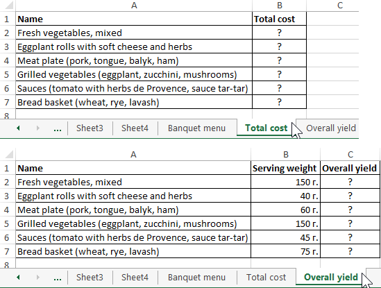
- Similarly, create tables on different sheets «Total cost» and «Total output»:
- Using the formula with links to other sheets, we will calculate the total cost of the banquet menu:
- Let’s go to the sheet “Total yield” and by multiplying the cells of the weight of one portion, located on sheet 2 and the total number, located on sheet 1, we will calculate the total output:
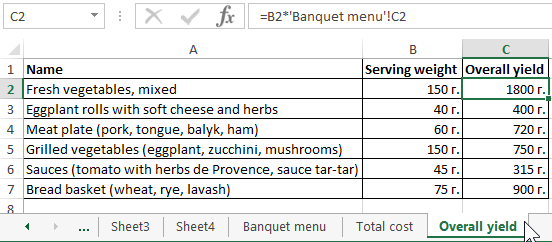
As a result, we got the simplest template for calculating the cost of 1 banquet.
Источник
How can I get a list of all the sheets that are in a file on one sheet?
Is there a way to find the names of all the sheets as a list?
I can find the sheet name of the sheet where the formula is placed in via the following formula:
This works for the sheet the formula is placed in. How can I get a list of all the sheets that are in a file on one sheet (let’s say in cell A1:A5 if I have 5 sheets)?
I would like to make it so when someone changes a sheet name the macro keeps working.
6 Answers 6
btw, in vba you can refer to worksheets by name or by object. See below, if you use the first method of referencing your worksheets it will always work with any name. 
I would keep a very hidden sheet with the formula you used referencing each sheet.
When the Workbook_NewSheet event fires a formula pointing to the new sheet is created:
- Create a sheet and give it the Code Name of shtNames .
- Give the sheet a tab name of SheetNames .
- In cell A1 of shtNames add a heading (I just used «Sheet List»).
- In Properties for the sheet change Visible to 2 — xlSheetVeryHidden.
You can only do this if there at least one visible sheet left.
- Add this code to the ThisWorkbook module:
Create a named range in the Name Manager:
- I called it SheetList .
- Use this formula:
=SheetNames!$A$2:INDEX(SheetNames!$A:$A,COUNTA(SheetNames!$A:$A))
You can then use SheetList as the source for Data Validation lists and list controls.
Two potential problems I haven’t looked at yet are rearranging the sheets and deleting the sheets.
so when someone changes a sheetname the macro keeps working
As @SNicolaou said though — use the sheet code name which the user can’t change and your code will carry on working no matter the sheet tab name.
Источник
Excel formula apply conditions to all sheets same whole column
This question can be viewed as several small ones , but the main aim is one and only .
TL;DR;
I would like to apply an excel formula at sheet N , that will take into consideration all the corresponding columns, in full, in all the other sheets, while applying some conditions that are the same for all columns .
Details :
My spreadsheet is a very simple and basic expenses accounting , which has many sheets by years and dates named 2015.04 , 2015.05 , 2015.06 etc. First row is always title ( time, date, amount , project, category etc. ) and the columns are always corresponding ( for example in all sheets column H will be category and D will be amount )
The starting formula is :
And it works at this simplified manual mode , but since we have computers, and I have a programmers M.O, I want to automate it a bit , and hence my problems :
1 — How to apply this formula to all sheets , even if some are later added / deleted , e.g. the equivalent of «sheet wildcard «
2 — Since the columns are not the same length , it is seems stupid to apply manual range , so I tried
But it gives me several different errors .
3 — ONE of the errors I can understand, and that is that the first row TITLE is not a number , so I tried
Now, I know I can take the simple working starting formula , put it in every single page, select the exact range without title, and then at the last summery page reference all the others — but seriously, I could also use an ABACUS , this is not why tools like excel were invented . or am I presuming too much of this tool ? is it that primitive ? I somehow refuse to believe it and just blame myself for not knowing it as well as I should .
I also know I can write a VBA macro, but at this point, it would take me much less effort and time to take some PHP excel library write some PHP lines , dump all in SQL and do it right . But again — is it my fault ( probably ) or excel’s ??
P.S>. Using OpenOffice Calc if that matters , but tried all also in excel with change of syntax and different error codes .
EDIT I — SOLUTION
After looking @Axel Richards answer, even if it not exactly helps me to resolve the problem, it did help me a lot in finding the way .
First, I found out that the errors I had were due to the naming of the sheets themselves . Apparently , a name like 2005.07 ( a dot ) will give err 501 and 2005-07 ( hyphen ) will give err 502 . That made me understand that some of my earlier attempt were actually right — but the naming scheme created the errors .
so the final formula, which works for me is . note that this is an array formula, and therefor needs to be entered with CTRL+SHIFT+ENTER and not just ENTER , which produces the curly brackets ( I did not know that before .. )
The fact that there are no wildcard, is only half correct, because the solution would be to define a starting period, and end period, and the formula will calculate all of thee sheets in the middle . That is some kind of a wildcard for my purposes.
The use of COLUMN(C$1:I$1) is actually to create an array ( 3-9 ) and the ROW(A$1:A$500) tells thee formula to take into account everything for 500 rows .
This is hardly a flexible or elegant solution, but it works .
Источник
Anyone who uses Excel will know that shortcuts and functions to make repetitive actions easier are very much welcomed. Therefore, in this article we will show you how to apply a formula to multiple sheets in Excel.
To apply a function to all or multiple sheets:
-
Firstly you need to select all sheets. To do this, click on the first tab (sheet) and then go on to the last tab while pressing Shift + Left click.
- All sheets should then be selected.
-
You can then type a function for a specific column, for example E3 and validate this function. It will then be applied to all cells in E3 on all sheets.
Need more help with Excel? Check out our forum!
SHEET function in Excel returns a numeric value corresponding to the sheet number referenced by the link passed to the function as a parameter.
SHEET and SHEETS functions in Excel: description of arguments and syntax
SHEETS function in Excel returns a numeric value that corresponds to the number of sheets referenced.
Notes:
- Both functions are useful for use in documents containing a large number of sheets.
- A sheet in Excel is a table of all the cells that are displayed on the screen and are outside of it (a total of 1,048,576 rows and 16,384 columns). When sending a sheet to print, it can be divided into several pages. Therefore, the terms “sheet” and “page” should not be confused.
- The number of sheets in the book is limited only by the amount of PC RAM.
Function has only 1 argument in its syntax and is optional for: =SHEET(value).
- value is an optional function argument that contains text data with the name of the sheet or a link for which you want to set the sheet number. If this parameter is not specified, the function will return the number of the sheet in one of the cells of which it was written.
Notes:
- When the sheet works, all sheets that are visible, hidden and very hidden are taken into account. Exceptions are dialogs, macros, and diagrams.
- If the function argument is a text value that does not match the name of any of the sheets contained in the book, the error #NA will be returned.
- If an invalid value was passed as an argument to the function, the result of its calculation will be the error #REF!.
- Within the object model (the hierarchy of objects in VBA, in which Application is the main object and Workbook, WorkSheet, etc., are child objects), the SHEET function is not available because it contains a similar function.
The function has the following syntax: =SHEETS(reference).
- reference — an object of reference type for which you want to determine the number of sheets. This argument is optional. If this parameter is not specified, the function will return the number of sheets contained in the book where it was written.
Notes:
- This function counts the number of all hidden, very hidden and visible sheets, with the exception of charts, macros and dialogs.
- If an invalid reference was passed as a parameter, the result of the calculation is the error code #REF!.
- This function is not available in the object model due to the presence of a similar function there.
How to get sheet name by formula in Excel
Example 1. In carrying out the calculated work the student used the Excel program, in which he created a book of several sheets. For his own convenience, the student decided to display in the cells A2 and B2 of each sheet data on the name of the sheet and its serial number, respectively. For this, he used the following formulas:
Description of arguments for the MID function:
- =CELL(«filename») is a function that returns text in which the MID function searches for a specified number of characters. In this case, the value “C:UserssoulpDesktop[Workbook.xlsx] Static_Calculations” will return, where after the “]” symbol is the required text — the name.
- =FIND(«]»,CELL(«filename»))+1 is a function that returns the position number of the character «]», one is added so that the MID function does not take into account the character].
- 31 — the maximum number of characters in the name.
=SHEET() — this function without parameter returns the number of the current sheet. As a result of its calculation, we get the number of sheets in the current book.
Examples of using the SHEET function and SHEETS
Example 2. The Excel workbook contains several sheets. It is necessary:
- Return the current sheet number.
- Return the sheet number with the name «Static_calculations».
- Return the number of the sheet «Dynamic_calculations», if its cell A3 contains the value 0.
Enter the data in the table:
Next, we write the formulas for all 4 conditions:
- For condition # 1, use the following formula: =SHEET()
- For condition # 2, enter the formula: =SHEET(«Static_calculations»)
- For condition number 3 we write the formula:
The IF function checks whether the value stored in the A3 cell of the Dynamic_ calculations is equal to zero or null.
As a result, we get:
Processing information about the sheets of the book on the formula Excel
Example 3. To determine the contains several sheets. It is necessary to determine the total number of sheets, as well as the number contained between the “Static_calculations” and “Economic_calculations”.
The source table is:
The total number of sheets is calculated by the formula:
To determine the number contained between these two sheets, we write the formula:
- Static_calculations: Economic_calculations!A2 — A reference to cell A2 of the range of sheets between «Static_calculations» and «Economic_calculations» including these sheets.
- To get the desired value, 2 was subtracted.
As a result, we get the following:
Download examples SHEET and SHEETS functions in Excel formulas
The formula displays detailed information on the data on the sheets in a certain range of their location in the Excel workbook.
If you have an Excel workbook that has hundreds of worksheets, and now you want to get a list of all the worksheet names, you can refer to this article. Here we will share 3 simple methods with you.
Sometimes, you may be required to generate a list of all worksheet names in an Excel workbook. If there are only few sheets, you can just use the Method 1 to list the sheet names manually. However, in the case that the Excel workbook contains a great number of worksheets, you had better use the latter 2 methods, which are much more efficient.
Method 1: Get List Manually
- First off, open the specific Excel workbook.
- Then, double click on a sheet’s name in sheet list at the bottom.
- Next, press “Ctrl + C” to copy the name.

- Later, create a text file.
- Then, press “Ctrl + V” to paste the sheet name.

- Now, in this way, you can copy each sheet’s name to the text file one by one.


Method 2: List with Formula
- At the outset, turn to “Formulas” tab and click the “Name Manager” button.
- Next, in popup window, click “New”.

- In the subsequent dialog box, enter “ListSheets” in the “Name” field.
- Later, in the “Refers to” field, input the following formula:

=REPLACE(GET.WORKBOOK(1),1,FIND("]",GET.WORKBOOK(1)),"")

- After that, click “OK” and “Close” to save this formula.
- Next, create a new worksheet in the current workbook.
- Then, enter “1” in Cell A1 and “2” in Cell A2.
- Afterwards, select the two cells and drag them down to input 2,3,4,5, etc. in Column A.

- Later, put the following formula in Cell B1.

=INDEX(ListSheets,A1)

- At once, the first sheet name will be input in Cell B1.
- Finally, just copy the formula down until you see the “#REF!” error.


Method 3: List via Excel VBA
- For a start, trigger Excel VBA editor according to “How to Run VBA Code in Your Excel“.
- Then, put the following code into a module or project.
Sub ListSheetNamesInNewWorkbook()
    Dim objNewWorkbook As Workbook
    Dim objNewWorksheet As Worksheet

    Set objNewWorkbook = Excel.Application.Workbooks.Add
    Set objNewWorksheet = objNewWorkbook.Sheets(1)

    For i = 1 To ThisWorkbook.Sheets.Count
        objNewWorksheet.Cells(i, 1) = i
        objNewWorksheet.Cells(i, 2) = ThisWorkbook.Sheets(i).Name
    Next i

    With objNewWorksheet
         .Rows(1).Insert
         .Cells(1, 1) = "INDEX"
         .Cells(1, 1).Font.Bold = True
         .Cells(1, 2) = "NAME"
         .Cells(1, 2).Font.Bold = True
         .Columns("A:B").AutoFit
    End With
End Sub

- Later, press “F5” to run this macro right now.
- At once, a new Excel workbook will show up, in which you can see the list of worksheet names of the source Excel workbook.


Comparison
| Advantages | Disadvantages | |
| Method 1 | Easy to operate | Too troublesome if there are a lot of worksheets |
| Method 2 | Easy to operate | Demands you to type the index first |
| Method 3 | Quick and convenient | Users should beware of the external malicious macros |
| Easy even for VBA newbies |
Excel Gets Corrupted
MS Excel is known to crash from time to time, thereby damaging the current files on saving. Therefore, it’s highly recommended to get hold of an external powerful Excel repair tool, such as DataNumen Outlook Repair. It’s because that self-recovery feature in Excel is proven to fail frequently.
Author Introduction:
Shirley Zhang is a data recovery expert in DataNumen, Inc., which is the world leader in data recovery technologies, including sql fix and outlook repair software products. For more information visit www.datanumen.com