
Excel for Microsoft 365 Excel for Microsoft 365 for Mac Excel for the web Excel 2021 Excel 2021 for Mac Excel 2019 Excel 2019 for Mac Excel 2016 Excel 2016 for Mac Excel 2013 Excel for iPad Excel for iPhone Excel for Android tablets Excel 2010 Excel 2007 Excel for Mac 2011 Excel for Android phones Excel Mobile More…Less
Unlike Microsoft Word, Microsoft Excel doesn’t have a Change Case button for changing capitalization. However, you can use the UPPER, LOWER, or PROPER functions to automatically change the case of existing text to uppercase, lowercase, or proper case. Functions are just built-in formulas that are designed to accomplish specific tasks—in this case, converting text case.
How to Change Case
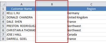
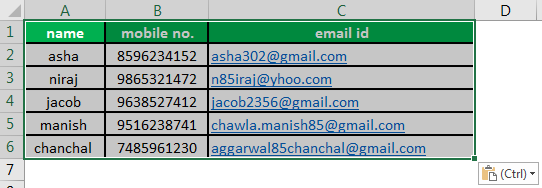
In the example below, the PROPER function is used to convert the uppercase names in column A to proper case, which capitalizes only the first letter in each name.
-
First, insert a temporary column next to the column that contains the text you want to convert. In this case, we’ve added a new column (B) to the right of the Customer Name column.

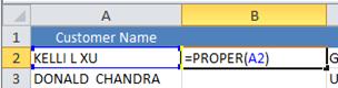
In cell B2, type =PROPER(A2), then press Enter.
This formula converts the name in cell A2 from uppercase to proper case. To convert the text to lowercase, type =LOWER(A2) instead. Use =UPPER(A2) in cases where you need to convert text to uppercase, replacing A2 with the appropriate cell reference.
-
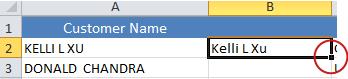
Now, fill down the formula in the new column. The quickest way to do this is by selecting cell B2, and then double-clicking the small black square that appears in the lower-right corner of the cell.
Tip: If your data is in an Excel table, a calculated column is automatically created with values filled down for you when you enter the formula.
-
At this point, the values in the new column (B) should be selected. Press CTRL+C to copy them to the Clipboard.
Right-click cell A2, click Paste, and then click Values. This step enables you to paste just the names and not the underlying formulas, which you don’t need to keep.
-
You can then delete column (B), since it is no longer needed.

Need more help?
You can always ask an expert in the Excel Tech Community or get support in the Answers community.
See Also
Use AutoFill and Flash Fill
Need more help?
Sign in with Microsoft
Sign in or create an account.
Hello,
Select a different account.
You have multiple accounts
Choose the account you want to sign in with.
Excel 2013
-
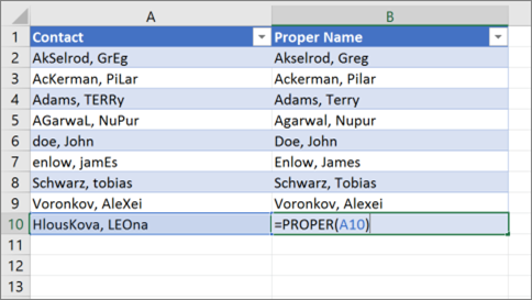
To change column A to Title Case, select cell B2. Type =PROPER(A2), and press Enter. Tip: Use the formula =UPPER(A1) for all UPPERCASE; =LOWER(A1) for all lowercase.
-
Now fill down the formula through cell B10.

Excel 2016
-
To change column A to Title Case, select cell B2. Type =PROPER(A2), and press Enter. Tip: Use the formula =UPPER(A1) for all UPPERCASE; =LOWER(A1) for all lowercase.
-
Now fill down the formula through cell B10.
Need more help?
Thank you for your feedback!
×
You’ve probably come across this situation before.
You have a list of names and it’s all lower case letter. You need to fix them so they are all properly capitalized.
With hundreds of names in your list, it’s going to be a pain to go through and edit first and last names.
Thankfully, there are some easy ways to change the case of any text data in Excel. We can change text to lower case, upper case or proper case where each word is capitalized.
In this post, we’re going to look at using Excel functions, flash fill, power query, DAX and power pivot to change the case of our text data.
Video Tutorial
Using Excel Formulas To Change Text Case
The first option we’re going to look at is regular Excel functions. These are the functions we can use in any worksheet in Excel.
There’s a whole category of Excel functions to deal with text, and these three will help us to change the text case.
LOWER Excel Worksheet Function
=LOWER(Text)The LOWER function takes one argument which is the bit of Text we want to change into lower case letters. The function will evaluate to text that is all lower case.
UPPER Excel Worksheet Function
=UPPER(Text)The UPPER function takes one argument which is the bit of Text we want to change into upper case letters. The function will evaluate to text that is all upper case.
PROPER Excel Worksheet Function
=PROPER(Text)The PROPER function takes one argument which is the bit of Text we want to change into proper case. The function will evaluate to text that is all proper case where each word starts with a capital letter and is followed by lower case letters.
Copy And Paste Formulas As Values
After using the Excel formulas to change the case of our text, we may want to convert these to values.
This can be done by copying the range of formulas and pasting them as values with the paste special command.
Press Ctrl + C to copy the range of cells ➜ press Ctrl + Alt + V to paste special ➜ choose Values from the paste options.
Using Flash Fill To Change Text Case
Flash fill is a tool in Excel that helps with simple data transformations. We only need to provide a couple examples of the results we want, and flash fill will fill in the rest.
Flash fill can only be used directly to the right of the data we’re trying to transform. We need to type out a couple of examples of the results we want. When Excel has enough examples to figure out the pattern, it will show the suggested data in a light grey font. We can accept this suggested filled data by pressing Enter.
We can also access flash fill from the ribbon. Enter the example data ➜ highlight both the examples and cells that need to be filled ➜ go to the Data tab ➜ press the Flash Fill command found in the Data Tools section.
We can also use the keyboard shortcut Ctrl + E for flash fill.
Flash fill will work for many types of simple data transformations including changing text between lower case, upper case and proper case.
Using Power Query To Change Text Case
Power query is all about data transformation, so it’s sure there is a way to change the case of text in this tool.
With power query we can transform the case into lower, upper and proper case.
Select the data we want to transform ➜ go to the Data tab ➜ select From Table/Range. This will open up the power query editor where we can apply our text case transformations.
Text.Lower Power Query Function
Select the column containing the data we want to transform ➜ go to the Add Column tab ➜ select Format ➜ select lowercase from the menu.
= Table.AddColumn(#"Changed Type", "lowercase", each Text.Lower([Name]), type text)This will create a new column with all text converted to lower case letters using the Text.Lower power query function.
Text.Upper Power Query Function
Select the column containing the data we want to transform ➜ go to the Add Column tab ➜ select Format ➜ select UPPERCASE from the menu.
= Table.AddColumn(#"Changed Type", "UPPERCASE", each Text.Upper([Name]), type text)This will create a new column with all text converted to upper case letters using the Text.Upper power query function.
Text.Proper Power Query Function
Select the column containing the data we want to transform ➜ go to the Add Column tab ➜ select Format ➜ select Capitalize Each Word from the menu.
= Table.AddColumn(#"Changed Type", "Capitalize Each Word", each Text.Proper([Name]), type text)This will create a new column with all text converted to proper case lettering, where each word is capitalized, using the Text.Proper power query function.
Using DAX Formulas To Change Text Case
When we think of pivot tables, we generally think of summarizing numeric data. But pivot tables can also summarize text data when we use the data model and DAX formulas. There are even DAX formula to change text case before we summarize it!
First, we need to create a pivot table with our text data. Select the data to be converted ➜ go to the Insert tab ➜ select PivotTable from the tables section.
In the Create PivotTable dialog box menu, check the option to Add this data to the Data Model. This will allow us to use the necessary DAX formula to transform our text case.
Creating a DAX formula in our pivot table can be done by adding a measure. Right click on the table in the PivotTable Fields window and select Add Measure from the menu.
This will open up the Measure dialog box, where we can create our DAX formulas.
LOWER DAX Function
=CONCATENATEX( ChangeCase, LOWER( ChangeCase[Mixed Case] ), ", ")We can enter the above formula into the Measure editor. Just like the Excel worksheet functions, there is a DAX function to convert text to lower case.
However, in order for the expression to be a valid measure, it will need to be wrapped in a text aggregating function like CONCATENATEX. This is because measures need to evaluate to a single value and the LOWER DAX function does not do this on it’s own. The CONCATENATEX function will aggregate the results of the LOWER function into a single value.
We can then add the original column of text into the Rows and the new Lower Case measure into the Values area of the pivot table to produce our transformed text values.
Notice the grand total of the pivot table contains all the names in lower case text separated by a comma and space character. We can hide this part by going to the Table Tools Design tab ➜ Grand Totals ➜ selecting Off for Rows and Columns.
UPPER DAX Function
=CONCATENATEX( ChangeCase, UPPER( ChangeCase[Mixed Case] ), ", ")Similarily, we can enter the above formula into the Measure editor to create our upper case DAX formula. Just like the Excel worksheet functions, there is a DAX function to convert text to upper case.
Creating the pivot table to display the upper case text is the same process as with the lower case measure.
Missing PROPER DAX Function
We might try and create a similar DAX formula to create proper case text. But it turns out there is no function in DAX equivalent to the PROPER worksheet function.
Using Power Pivot Row Level Formulas To Change Text Case
This method will also use pivot tables and the Data Model, but instead of DAX formulas we can create row level calculations using the Power Pivot add-in.
Power pivot formulas can be used to add new calculated columns in our data. Calculations in these columns happen for each row of data similar to our regular Excel worksheet functions.
Not every version of Excel has power pivot available and you will need to enable the add-in before you can use it. To enable the power pivot add-in, go to the File tab ➜ Options ➜ go to the Add-ins tab ➜ Manage COM Add-ins ➜ press Go ➜ check the box for Microsoft Power Pivot for Excel.
We will need to load our data into the data model. Select the data ➜ go to the Power Pivot tab ➜ press the Add to Data Model command.
This is the same data model as creating a pivot table and using the Add this data to the Data Model checkbox option. So if our data is already in the data model we can use the Manage data model option to create our power pivot calculations.
LOWER Power Pivot Function
=LOWER(ChangeCase[Mixed Case])Adding a new calculated column into the data model is easy. Select an empty cell in the column labelled Add Column then type out the above formula into the formula bar. You can even create references in the formula to other columns by clicking on them with the mouse cursor.
Press Enter to accept the new formula.
The formula will appear in each cell of the new column regardless of which cell was selected. This is because each row must use the same calculation within a calculated column.
We can also rename our new column by double clicking on the column heading. Then we can close the power pivot window to use our new calculated column.
When we create a new pivot table with the data model, we will see the calculated column as a new available field in our table and we can add it into the Rows area of the pivot table. This will list out all the names in our data and they will all be lower case text.
UPPER Power Pivot Function
=UPPER(ChangeCase[Mixed Case])We can do the same thing to create a calculated column that converts the text to upper case by adding a new calculated column with the above formula.
Again, we can then use this as a new field in any pivot table created from the data model.
Missing PROPER Power Pivot Function
Unfortunately, there is no power pivot function to convert text to proper case. So just like DAX, we won’t be able to do this in a similar fashion to the lower case and upper case power pivot methods.
Conclusions
There are many ways to change the case of any text data between lower, upper and proper case.
- Excel Formulas are quick, easy and will dynamically update if the inputs ever change.
- Flash fill is great for one-off transformations where you need to quickly fix some text and don’t need to update or change the data after.
- Power query is perfect for fixing data that will be imported regularly into Excel from an outside source.
- DAX and power pivot are can be used for fixing text to display within a pivot table.
Each option has different strengths and weaknesses so it’s best to become familiar will all methods so you can choose the one that will best suit your needs.
About the Author
John is a Microsoft MVP and qualified actuary with over 15 years of experience. He has worked in a variety of industries, including insurance, ad tech, and most recently Power Platform consulting. He is a keen problem solver and has a passion for using technology to make businesses more efficient.
Top 6 Methods to Change Capital Letters to Lower Case
There are many methods to change capital letter text to lowercase in Excel. This guide will look at the top 6 ways to make capital letters into lower cases.
Table of contents
- Top 6 Methods to Change Capital Letters to Lower Case
- #1 Using Lower Function to change case in Excel
- Example
- #2 Using VBA Command Button
- Example
- #3 Using VBA Shortcut key
- Example
- #4 Using Flash Fill
- Example
- #5 Enter Text in Lower Case Only
- Example
- #6 Using Microsoft Word
- Example
- Things to Remember
- Recommended Articles
- #1 Using Lower Function to change case in Excel
You can download this LowerCase Excel Template here – LowerCase Excel Template
#1 Using Lower Function to change case in Excel
MS Excel has a built-in function for decapitalizing each character in a word, a LOWER function.
Example
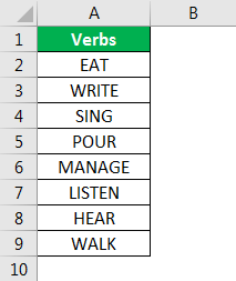
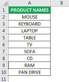
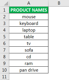
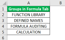
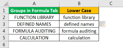
Suppose we have a list of some verbs in Excel. We want to change the case of the text to lowercase.
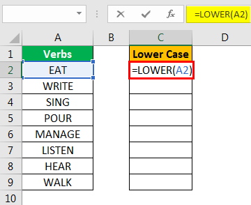
To change the case to lower, we need to write the function in cell C2 as ‘=LOWER(A2)’. The”=’ or ‘+’ sign is used to write the function, the “LOWER” is the function name, and A2 is the cell referenceCell reference in excel is referring the other cells to a cell to use its values or properties. For instance, if we have data in cell A2 and want to use that in cell A1, use =A2 in cell A1, and this will copy the A2 value in A1.read more for the text we want to change the case.
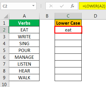
Press the “Enter” key. This function will convert all letters in a text string to lowercase.
One value is converted now. For other values, we can either press the “Ctrl+D” key after selecting all the cells with the top cell or press the “Ctrl+C” and “Ctrl+V” for copying and pasting the function. Else, we can drag the formula to other cells to get the answer.
#2 Using VBA Command Button
We can create a VBA command button and assign the code to change the following text to lowercase using the command button.
Example
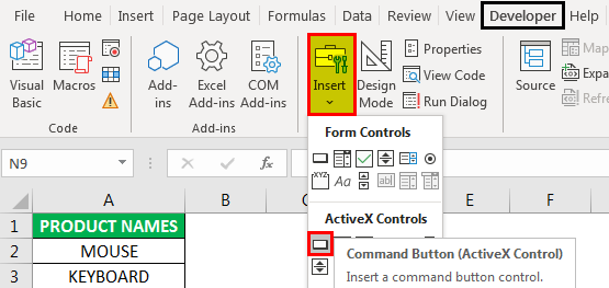
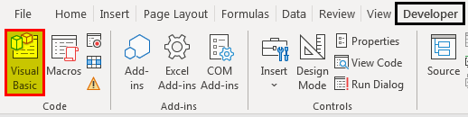
Step 1: To create the command button, click on the “Insert” command in the “Controls” group in ‘Developer tab ExcelEnabling the developer tab in excel can help the user perform various functions for VBA, Macros and Add-ins like importing and exporting XML, designing forms, etc. This tab is disabled by default on excel; thus, the user needs to enable it first from the options menu.read more.’ And select the “Command Button.”
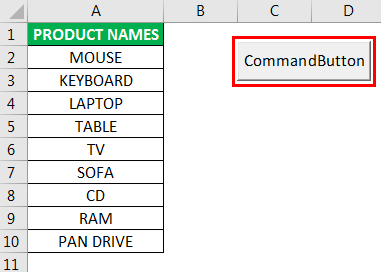
Step 2: Click the worksheet location where we want the command button to appear. We can resize the command button using the “ALT” button.
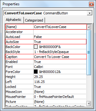
Step 3: Using the “Properties” command, change the properties of the command button like caption, name, AutoSize, WordWrap, etc.
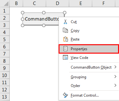
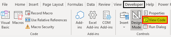
Step 4: To assign the code to the command button, we must click on the “View Code” command in the “Controls” group in the “Developer” tab. Ensure “Design Mode” is activated.
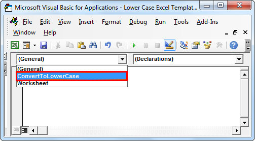
Step 5: Please select “ConvertToLowerCase” from the drop-down list in the opened window.
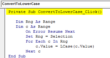
Step 6: Paste the following code in between the lines.
Code:
Dim Rng As Range
Dim c As Range
    On Error Resume Next
    Set Rng = Selection
    For Each c In Rng
        c.Value = LCase(c.Value)
    Next c
Step 7: Exit the Visual Basic Editor. Ensure the file is saved with the .xlsm extension as we have a macro in the workbook.
Step 8: Now, deactivate “Design Mode.” After selecting the required cells, the values are converted to lowercase whenever we click on the command button.
Select all the values from A2:A10 and click on the command button. The text will get changed to lowercase.
#3 Using the VBA Shortcut key
This way is similar to the above, except we do not need to create the command button here.
Example
Step 1: Open the Visual Basic Editor from the “Developer” tab or use using the excel shortcut keyAn Excel shortcut is a technique of performing a manual task in a quicker way.read more (Alt+ F11).
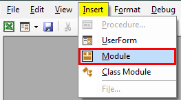
Step 2: Insert the module using the Insert menu -> Module command.
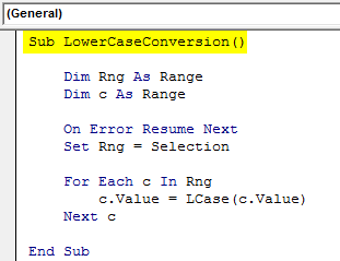
Step 3: Paste the following code.
Sub LowerCaseConversion()

    Dim Rng As Range
    Dim c As Range

    On Error Resume Next
    Set Rng = Selection

    For Each c In Rng
        c.Value = LCase(c.Value)
    Next c

End Sub
Step 4: Save the file using Ctrl+S. Exit the visual basic editorThe Visual Basic for Applications Editor is a scripting interface. These scripts are primarily responsible for the creation and execution of macros in Microsoft software.read more. Ensure the file is saved with the .xlsm extension as we have a macro in our workbook.
Step 5: Now, choose the “Macros” in the “Code” group in the “Developer” tab.
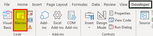
Step 6: Then click on “Options” and assign the shortcut key to the macro. We can write a description as well.
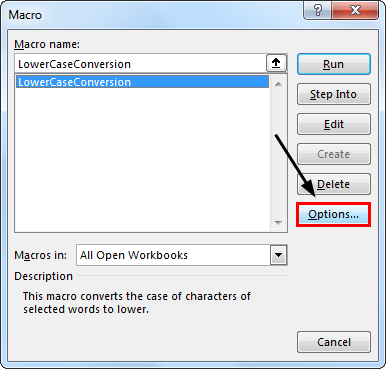
In our case, we have been assigned “Ctrl+Shift+L.”
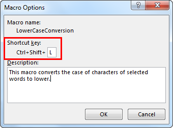
Step 7: Macro is ready to use. Select the required cells to change the values into lowercase and press the “Ctrl+Shift+L” keys.
#4 Using Flash Fill
If we establish a pattern by typing the same value in the lowercase in the adjacent column, the Flash FillAutomatic fillers in the cells of an excel table are known as flash fills. When you type certain characters in the adjacent cells, the suggested data appears automatically. It can be found under the data tab’s data tools section or by pressing CTRL + E on the keyboard.read more feature will fill in the rest based on the design we provide. Let us understand this with an example.
Example
Suppose we have the following data, which we want to get in lowercase.
We need to manually write the first list value in the lower case in the adjacent cell to do the same.

Come to the next cell in the same column and press the “Ctrl+E” keys.

Choose “Accept Suggestions” from the box menu that appeared.
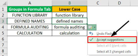
That is it. We have all the values in the lower case now. So, we can copy the values, paste the same onto the original list, and delete the extra value from the right.
#5 Enter Text in Lower Case Only
We can make a restriction so that the user can enter text values in lowercase only.
Example
To do this, the steps are:
- We must select the cells which we want to restrict.
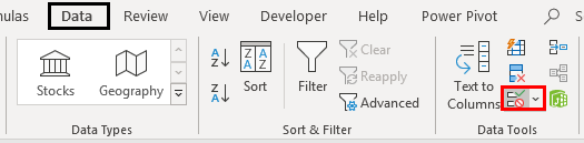
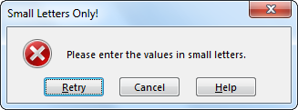
- Then, choose “Data Validation” from the “Data Tools” group from the “Data” tab.
- Apply the settings explained in the figure below.
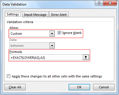
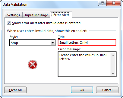
- Whenever the user enters the value in capital letters, MS Excel will stop and show the following message.
#6 Using Microsoft Word
In Microsoft Word, unlike Excel, we have a command named “Change Case” in the “Font” group in the “Home” tab.
Example
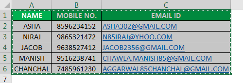
Suppose we have the following data table for which we want to change the text case to the “lower” case.
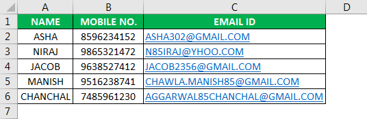
First, we will copy the data from MS Excel and paste it into MS Word to change the case. To do the same, the steps are:
Select the data from MS Excel. And press the “Ctrl+C” key to copy data from MS Excel.
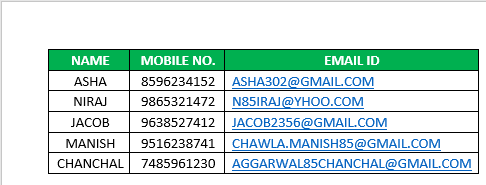
Open the MS Word application and paste the table using the “Ctrl+V” shortcut key.
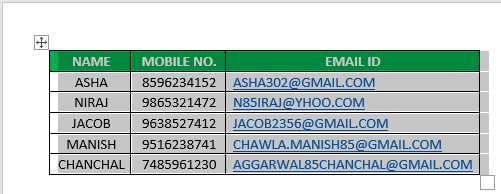
Select the table using the “Plus” sign on the left-top side of the table.
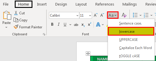
Choose the “Change Case” command from the “Font” group and select “lowercase” from the list.
Now, the data table is converted to “Lower.” After selecting the “Plus” sign from the left top corner, we can copy the table and paste it into Excel.
We can delete the old table using the “Contextual” menu, which we can get by right-clicking on the table.
Things to Remember
Using the VBA code (command button or shortcut key) to convert the values into lowercase, we must save the file with the .xlsm extension as we have macros in the workbook.
Recommended Articles
This article is a guide to Lowercase in Excel. We discuss the top 6 ways to change capital letters to the lower cases, including – the LOWER function, VBA Code, Flash Fill, VBA shortcut keys, etc., along with examples. You can learn more about Excel functions from the following articles: –
- Switch Case using VBA
- Case Statement in VBA
- Uppercase in Excel
- UCase Function in VBA
Method #1: Using Formulas
The main advantage to using formulas is that if the source data changes, the updated formula version automatically updates.
In our data set, we have a list of names with a variety of issues. Some names are lower case, some are upper case, some are proper case, and some are mixed up beyond all reason.

We will create a version of each name in the list to upper case, lower case, and proper case using formulas. Each of these methods are incredibly simple.
Upper Case
The function to convert any cell’s text to upper case is known as the UPPER function. The syntax for the UPPER function is as follows:
=UPPER(text)The variable “text” can refer to a cell address or to a statically declared string.
=UPPER(A1)or
=UPPER(“This is a test of the upper function”)In most cases, the cell reference version is the most useful option of the two.
In our sample file, we will select cell B5 and enter the following formula:
=UPPER(A5)
Fill the formula down column B to finish converting the list in column A.

If you don’t want the formulas in the resultant cells, you just want the new upper-cased versions of the names as if they had been hand-typed, you can select the names and perform a Copy -> Past Values operation on them.

A lesser-know technique to converting formulas to the formula’s results is to do the following:
- highlight the desired cells to be converted
- using your RIGHT mouse button, right-click on the thick, green border surrounding the selection
- drag a small amount away form the selection and then immediately return to the original selection location
- release your right mouse button
This presents you with a menu of choices. The choice we want is labeled “Copy Here as Values Only”.

Lower Case
The function to convert any cell’s text to upper case is known as the LOWER function. The syntax for the LOWER function is as follows:
=LOWER(text)The variable “text” can refer to a cell address or to a statically declared string.
=LOWER(A1)or
=LOWER(“THIS IS A TEST OF THE LOWER FUNCTION”)As with the UPPER function, the cell reference version is the most useful option of the two.
In our sample file, we will select cell C5 and enter the following formula:
=LOWER(A5)
Fill the formula down column C to finish converting the list in column A.

Proper Case
The function to convert any cell’s text to upper case is known as the PROPER function. The syntax for the PROPER function is as follows:
=PROPER(text)The variable “text” can refer to a cell address or to a statically declared string.
=PROPER(A1)or
=PROPER(“THIS IS A TEST OF THE PROPER FUNCTION”)In our sample file, we will select cell D5 and enter the following formula:
=PROPER(A5)
Fill the formula down column D to finish converting the list in column A.

Bonus Problem to Solve
Notice in our solution columns (B:D), “James Willard” has an extra space between his first and last names.

A less obvious issue is that “Gary Miller” has an extra space at the end of his name.

If you need to remove any unnecessary leading spaces, trailing spaces, or multiple spaces in between words, you can use the TRIM function. The syntax for the TRIM function is as follows:
=TRIM(text)The variable “text” can refer to a cell address or to a statically declared string.
=TRIM(A1)or
= TRIM(“ This is a test of the TRIM function ”)In our sample file, we will select cell E5 and enter the following formula:
=TRIM(A5)
Fill the formula down column E to finish converting the list in column A.
We can combine these functions to both trim and fix text casing. Suppose we wish to convert the text to upper case and trim all the extraneous spaces. We can write the formula two different ways.
=UPPER(TRIM(A3))or
=TRIM(UPPER(A3))Either version produces the desired results. Pick the one that makes the most sense to your brain.
Method #2: Flash Fill
The advantage of Flash Fill is that it doesn’t require the use of functions and the result is like the Copy -> Paste Values action in that the result cells contain the text, not formulas.
The disadvantage is that there is no dynamic connection back to the original list of text. If the original list changes, the “fixed” version of the list does not update. This is okay if you have a static list or you only need to perform the conversion one time and you don’t require updates.
There are many ways to use Flash Fill, but a simple way is to type on the same row as the data a version of the data as you WISH it were formatted.

After you press ENTER to commit the new version to a cell, press the keyboard combination CTRL-E.

The system will look for patterns in what you typed against other text on the same row. If a pattern exists, such as “I see the text you typed, but you typed it in upper case letters”, the system will repeat the pattern for the remainder of the rows in the table.
The Flash Fill tool can also be activated by selecting Home (tab) -> Editing (group) -> Fill (button) -> Flash Fill.

Another way to activate the Flash Fill tool is to select Data (tab) -> Data Tools (group) -> Flash Fill.

If we use the Flash Fill technique to convert the names in column A to upper case version in column B, notice that “James Willard” still has the extra space between his names.
Flash Fill can fix that problem as well. Flash Fill can perform the TRIM and the UPPER functions simultaneously. The trick is to select a name that contains extra spaces before, after, or within itself. In this case, we will use “james willard”.
In cell B4, type “JAMES WILLARD” with only a single space separating the first from the last name.

After you press ENTER, press the keyboard combination CTRL-E.
Flash Fill will fix the names in BOTH directions of the list. Not only will it create upper case versions of the names, but it is smart enough to detect that you only placed a single space between the names and that it should do the same thing. Also, because you didn’t add any additional leading or training spaces, Flash Fill doesn’t place any in the results list of names.
Although Flash Fill is a fantastic tool that can quickly correct may data entry mishaps, it isn’t perfect. If there isn’t a recognizable pattern, or if it perceives multiple patterns, it may produce unexpected results. It’s always a good idea to double-check the output of Flash Fill for accuracy.
Method #3: ALL CAPS FONT
The advantage of this method is lack of composing any formulas or using Flash Fill.
Imagine a scenario where you always want a page title to be in upper case, but you don’t want to worry about how the user type the title. If the user enters the title in lower case, proper case, or sentence case, we want the typed text to automatically convert to upper case.
We can accomplish this by using a font that contains no lower case version of the letters.
When you are browsing through your list of fonts, you can tell if a font is upper case only because the font name will be in all upper case letters.

Some of the supplied fonts in Microsoft Windows/Office that contain only upper case letters are:
- Copperplate Gothic
- Engravers
- Felix Tilting
- Stencil
You are not restricted to fonts that came with Windows or Office. Many websites exist that provide both free and “pay-to-play” fonts.
- WebsitePlant.com
- 1001freefonts.com
- dafont.com
- fontsquirrel.com
When you are downloading a font from one of these sites, or other font supplier’s sites, be mindful that some fonts are free for personal use, but other fonts may require a fee when used in a business capacity.
When you download and install the font based on the website’s installation instructions, the font will be available to all your Windows and Office applications, not just Excel.
Using the Newly Installed Font
With the font installed, we return to Excel and select a cell where we will enter our title.
From the font dropdown list, select the desired font that contains all upper case letters.

It doesn’t matter weather you type your title in upper case, lower case, or mixed case, the result will always be in an upper case format.

Using Cell Styles to Expedite Font Assignment
Locating a specific font for all for all your titles can be time consuming, especially if you must repeatedly scroll through long list of font choices.
A timesaving way to apply an ALL CAPS font to a cell is to utilize Cell Styles.
Cell Styles are located on the Home tab in the Styles group.

You have the option to use an existing style, create your own style and add it to the library, or modify an existing style.
If we wish to use the Heading 1 style, but we wish it to be in all upper case letters, right-click on the Heading 1 style and select Modify.

In the Style dialog box, click the Format button.

In the Format Cells dialog box, select the Font tab and set the font to the desired ALL CAPS font. You can also use this opportunity to set the font color, underline color, border color, etc…

We can now select a cell and type in our new title. Once entered, with the title cell selected, click the Heading 1 style from the Cell Styles list.

Practice Workbook
Feel free to Download the Workbook HERE.
![]()
Published on: April 5, 2019
Last modified: March 2, 2023


Leila Gharani
I’m a 5x Microsoft MVP with over 15 years of experience implementing and professionals on Management Information Systems of different sizes and nature.
My background is Masters in Economics, Economist, Consultant, Oracle HFM Accounting Systems Expert, SAP BW Project Manager. My passion is teaching, experimenting and sharing. I am also addicted to learning and enjoy taking online courses on a variety of topics.