Excel all formulas to values - Word и Excel - помощь в работе с программами

Replace formulas with their calculated values

When you replace formulas with their values, Excel permanently removes the formulas. If you accidentally replace a formula with a value and want to restore the formula, click Undo immediately after you enter or paste the value.

Select the cell or range of cells that contains the formulas.

If the formula is an array formula, select the range that contains the array formula.

How to select a range that contains the array formula
1. Click a cell in the array formula.
2. On the Home tab, in the Editing group, click Find & Select, and then click Go To.
3. Click Special.
4. Click Current array.
Click Copy .
Click Paste .
Click the arrow next to Paste Options , and then click Values Only.

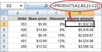
The following example shows a formula in cell D2 that multiplies cells A2, B2, and a discount derived from C2 to calculate an invoice amount for a sale. To copy the actual value instead of the formula from the cell to another worksheet or workbook, you can convert the formula in its cell to its value by doing the following:

Press F2 to edit the cell.
Press F9, and then press ENTER.

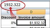
After you convert the cell from a formula to a value, the value appears as 1932.322 in the formula bar. Note that 1932.322 is the actual calculated value, and 1932.32 is the value displayed in the cell in a currency format.

Tip: When you are editing a cell that contains a formula, you can press F9 to permanently replace the formula with its calculated value.

Replace part of a formula with its calculated value

There may be times when you want to replace only a part of a formula with its calculated value. For example, you want to lock in the value that is used as a down payment for a car loan. That down payment was calculated based on a percentage of the borrower’s annual income. For the time being, that income amount won’t change, so you want to lock the down payment in a formula that calculates a payment based on various loan amounts.

When you replace a part of a formula with its value, that part of the formula cannot be restored.

Click the cell that contains the formula.
In the formula bar , select the portion of the formula that you want to replace with its calculated value. When you select the part of the formula that you want to replace, make sure that you include the entire operand. For example, if you select a function, you must select the entire function name, the opening parenthesis, the arguments, and the closing parenthesis.
To calculate the selected portion, press F9.
To replace the selected portion of the formula with its calculated value, press ENTER.

In Excel for the web the results already appear in the workbook cell and the formula only appears in the formula bar .

Источник

Преобразование формул в значения

Формулы – это хорошо. Они автоматически пересчитываются при любом изменении исходных данных, превращая Excel из «калькулятора-переростка» в мощную автоматизированную систему обработки поступающих данных. Они позволяют выполнять сложные вычисления с хитрой логикой и структурой. Но иногда возникают ситуации, когда лучше бы вместо формул в ячейках остались значения. Например:

Вы хотите зафиксировать цифры в вашем отчете на текущую дату.
Вы не хотите, чтобы клиент увидел формулы, по которым вы рассчитывали для него стоимость проекта (а то поймет, что вы заложили 300% маржи на всякий случай).
Ваш файл содержит такое больше количество формул, что Excel начал жутко тормозить при любых, даже самых простых изменениях в нем, т.к. постоянно их пересчитывает (хотя, честности ради, надо сказать, что это можно решить временным отключением автоматических вычислений на вкладке Формулы – Параметры вычислений).
Вы хотите скопировать диапазон с данными из одного места в другое, но при копировании «сползут» все ссылки в формулах.

В любой подобной ситуации можно легко удалить формулы, оставив в ячейках только их значения. Давайте рассмотрим несколько способов и ситуаций.

Способ 1. Классический

Этот способ прост, известен большинству пользователей и заключается в использовании специальной вставки:

Выделите диапазон с формулами, которые нужно заменить на значения.
Скопируйте его правой кнопкой мыши – Копировать (Copy).
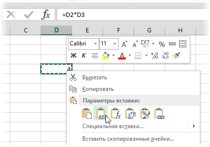
Щелкните правой кнопкой мыши по выделенным ячейкам и выберите либо значок Значения (Values):

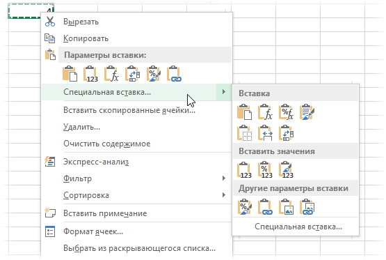
либо наведитесь мышью на команду Специальная вставка (Paste Special), чтобы увидеть подменю:

Из него можно выбрать варианты вставки значений с сохранением дизайна или числовых форматов исходных ячеек.

В старых версиях Excel таких удобных желтых кнопочек нет, но можно просто выбрать команду Специальная вставка и затем опцию Значения (Paste Special — Values) в открывшемся диалоговом окне:

Способ 2. Только клавишами без мыши

При некотором навыке, можно проделать всё вышеперечисленное вообще на касаясь мыши:

Копируем выделенный диапазон Ctrl+C
Тут же вставляем обратно сочетанием Ctrl+V
Жмём Ctrl, чтобы вызвать меню вариантов вставки
Нажимаем клавишу с русской буквой З или используем стрелки, чтобы выбрать вариант Значения и подтверждаем выбор клавишей Enter:

Способ 3. Только мышью без клавиш или Ловкость Рук

Этот способ требует определенной сноровки, но будет заметно быстрее предыдущего. Делаем следующее:

Выделяем диапазон с формулами на листе
Хватаем за край выделенной области (толстая черная линия по периметру) и, удерживая ПРАВУЮ клавишу мыши, перетаскиваем на пару сантиметров в любую сторону, а потом возвращаем на то же место
В появившемся контекстном меню после перетаскивания выбираем Копировать только значения (Copy As Values Only).

После небольшой тренировки делается такое действие очень легко и быстро. Главное, чтобы сосед под локоть не толкал и руки не дрожали

Способ 4. Кнопка для вставки значений на Панели быстрого доступа

Ускорить специальную вставку можно, если добавить на панель быстрого доступа в левый верхний угол окна кнопку Вставить как значения. Для этого выберите Файл — Параметры — Панель быстрого доступа (File — Options — Customize Quick Access Toolbar). В открывшемся окне выберите Все команды (All commands) в выпадающем списке, найдите кнопку Вставить значения (Paste Values) и добавьте ее на панель:

Теперь после копирования ячеек с формулами будет достаточно нажать на эту кнопку на панели быстрого доступа:

Кроме того, по умолчанию всем кнопкам на этой панели присваивается сочетание клавиш Alt + цифра (нажимать последовательно). Если нажать на клавишу Alt, то Excel подскажет цифру, которая за это отвечает:

Способ 5. Макросы для выделенного диапазона, целого листа или всей книги сразу

Если вас не пугает слово «макросы», то это будет, пожалуй, самый быстрый способ.

Макрос для превращения всех формул в значения в выделенном диапазоне (или нескольких диапазонах, выделенных одновременно с Ctrl) выглядит так:

Sub Formulas_To_Values_Selection()
'преобразование формул в значения в выделенном диапазоне(ах)
    Dim smallrng As Range
    For Each smallrng In Selection.Areas
        smallrng.Value = smallrng.Value
    Next smallrng
End Sub

Если вам нужно преобразовать в значения текущий лист, то макрос будет таким:

Sub Formulas_To_Values_Sheet()
'преобразование формул в значения на текущем листе
    ActiveSheet.UsedRange.Value = ActiveSheet.UsedRange.Value
End Sub

И, наконец, для превращения всех формул в книге на всех листах придется использовать вот такую конструкцию:

Sub Formulas_To_Values_Book()
'преобразование формул в значения во всей книге
    For Each ws In ActiveWorkbook.Worksheets
        ws.UsedRange.Value = ws.UsedRange.Value
    Next ws
End Sub

Код нужных макросов можно скопировать в новый модуль вашего файла (жмем Alt+F11 чтобы попасть в Visual Basic, далее Insert — Module). Запускать их потом можно через вкладку Разработчик — Макросы (Developer — Macros) или сочетанием клавиш Alt+F8. Макросы будут работать в любой книге, пока открыт файл, где они хранятся. И помните, пожалуйста, о том, что действия выполненные макросом невозможно отменить — применяйте их с осторожностью.

Способ 6. Для ленивых

Если ломает делать все вышеперечисленное, то можно поступить еще проще — установить надстройку PLEX, где уже есть готовые макросы для конвертации формул в значения и делать все одним касанием мыши:

В этом случае:

всё будет максимально быстро и просто
можно откатить ошибочную конвертацию отменой последнего действия или сочетанием Ctrl+Z как обычно
в отличие от предыдущего способа, этот макрос корректно работает, если на листе есть скрытые строки/столбцы или включены фильтры
любой из этих команд можно назначить любое удобное вам сочетание клавиш в Диспетчере горячих клавиш PLEX

Ссылки по теме

Что такое макросы, как их использовать, копировать и запускать
Как скопировать формулы без сдвига ссылок
Как считать в Excel без формул

Источник

Watch Video – Convert Formulas to Values (Remove Formulas but Keep the data)

You may need to convert formulas to Values in Excel if you work with a lot of dynamic or volatile formulas.

For example, if you use Excel TODAY function to insert the current date in a cell, and you leave it as a formula, it will update itself if you open the workbook the next day. If this is not what you want, then you need to convert the formula into a static value.

Convert Formulas to Values in Excel

In this tutorial, I will show you various ways to convert formulas to values in Excel.

Using a Keyboard Shortcut.
Using Paste Special techniques.
Using a cool Mouse Wriggle Trick.

Using Keyboard Shortcut

This is one of the easiest ways to convert formulas to values. A simple keyboard shortcut trick.

Here is how to do this:

Select the cells for which you want to convert formulas to values.
Copy the cells (Control + C).
Paste as Values – Keyboard Shortcut – ALT + ESV

This would instantly convert all the formulas into static values.

Caution: When you do this, you lose all the original formulas. If you think you may need the formulas at a later stage, make a copy of the worksheet as back-up.

Using Paste Special

If you are not a keyboard shortcuts fan, you can use the paste special option that can be accessed from the ribbon in Excel.

Here are the steps to convert formulas to values using Paste Special:

Select the cells for which you want to convert formulas to values.
Copy the cells (Control + C).
Go to Home –> Clipboard –> Paste –> Paste Special.

You can also access the same paste special option if you right click on the copied cell. Hover your mouse on the Paste Special option and you will all the options within it.

Using a Mouse Wriggle Trick

This is one mouse trick that not many people would know.

Here it is:

Select the cells for which you want to convert formulas to values.
Bring your mouse cursor over the outline of the selected cells. (You will see an icon of four arrows pointing in the four directions).
Press the RIGHT button of your mouse. Hold the button and drag the outline to the right and bring it back to its original position. As soon as you leave the mouse button, a menu would appear.
Click on Copy Here as Values only.
That’s it. It will instantly convert formulas to values in the selected cells.

Hope you found this tutorial useful.

Let me know your thoughts in the comments section.

You May Also Like the Following Excel Tutorials:

How to Multiply in Excel Using Paste Special.
How to Lock formulas in Excel.
Keyboard & Mouse Tricks that will Reinvent the Way You Excel.
Boost Your Productivity with Excel Mouse Double Click Tricks.
Understanding Absolute, Relative, and Mixed Cell References in Excel
How to Convert Numbers to Text in Excel

Источник

Hello Excellers and welcome back to another blog post of #ExcelTips in my 2019 #FormulaFriday series. Today let’s look at 4 ways to convert cells with formulas to values. So you are probably thinking when would I make use of this then?. Well, how about if your worksheet contains a lot of volatile formulas or lots of array formulas. These will degrade the performance of your workbook?. You workbook maybe the full and final presentation. It needs no further amending. Or you simply just do not want anyone to see your formulas!. So, whatever your reason, I will share with you my top 4 Excel Tips for converting formulas to values in Excel.

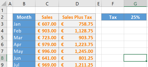
I have a sample of data. So, we will use the same data for all the methods I am about to share with you. It is a simple set of sales values with a sales+ tax calculation.

Convert Formulas To Values In Excel.

Method 1. Paste Special.

Yes, that is correct, the good old Paste Special method. Follow the steps below.

Select the range of cells that contain the formulas you want to convert to values. In this example, it is D2:D9.
Right-Click the mouse to copy the values.
Right- Click again to access the Paste Special options and select Values
Or, Home Tab | Clipboard | Paste Special | Values.

Paste Special To Convert Formulas To Values.

Method 2. Right-Click Drag and Drop.

If you want to avoid using the Paste Special method then this one may be for you. It’s a neat and quick way to convert formulas to values. We will use the same data set as in Method 1.

Select the range of cells with your formulas.
Right- Click on the edge of your selection of cells.
Hold the Right – Click on your cells. Next, move your selection to the right and bring it straight back to its original position and drop it.
A menu will appear, you need to select Copy Here As Values Only.

Drag And Drop To Convert Formulas To Values

Method 3. Using A Keyboard Shortcut.

If you are a fan of Excel keyboard shortcuts then this is the method for you. Using keyboard shortcuts to convert your Excel formulas to values.

Select the range of cells that you want to convert to values.
Hit Ctrl+C to copy those cells.
Press Alt+E S V
This is will replace all formulas with their values.

Method 4. Using VBA (Macro).

So, my final method uses some simple Excel VBA code. With just a few lines of code, we can write our own Excel macro. How cool is that?

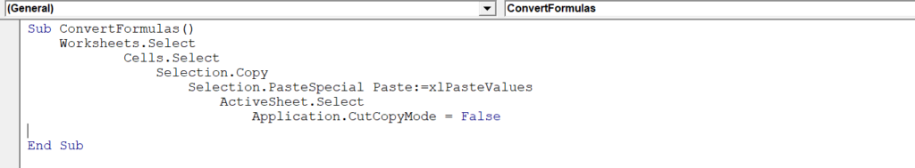
This macro will convert ALL formulas in an Excel worksheet to values on our Excel worksheet.

A Macro To Convert all formulas To Values

Open the Visual Basic Editor. You can do this by either selecting the Developer Tab | Code | Visual Basic. Alternatively, you can hit ALT+F11 as a shortcut to open the Visual Basic Editor window.
Decide where you want to save your Excel code. If we want to use this code only in this workbook then we need to insert a new module into this workbook. If we want to use this code in ANY workbook then we can create a module in the Personal Macro Workbook. I invite you to read my blog posts relating to the Personal Macro Workbook below. Saving it in this specific workbook makes your code available to any Excel workbook you use.
We select all of the cells in all of our worksheets in our workbook. (Worksheets. Select coding will select all worksheets in the current workbook).
Excel uses the PasteSpecial Paste:=xlPasteValues command to paste the value only back into the cells of the worksheets.
Test your Macro!.

That is all there is to this piece of code. Save this in your Personal Macro Workbook. If you do this it will be to hand if you need to convert ALL formulas in ALL worksheets in your current workbook. A quick rough and ready Excel VBA Macro!

What Next? Want More Tips?

So, if you want more top tips then sign up for my Monthly Newsletter where I share 3 Tips on the first Wednesday of the month and receive my free Ebook, 30 Excel Tips.

Do You Need Help With An Excel Problem?.

I am pleased to announce I have teamed up with Excel Rescue, where you can get help FAST.

Udemy.com Home page 125x125

Источник

Содержание

How to convert formulas to values
Related functions
Transcript
Replace a formula with its result
Replace formulas with their calculated values
Replace part of a formula with its calculated value
Need more help?
How to Convert Formulas to Values in Excel
Преобразование формул в значения
Способ 1. Классический
Способ 2. Только клавишами без мыши
Способ 3. Только мышью без клавиш или Ловкость Рук
Способ 4. Кнопка для вставки значений на Панели быстрого доступа
Способ 5. Макросы для выделенного диапазона, целого листа или всей книги сразу
Способ 6. Для ленивых

How to convert formulas to values

Transcript

As you start to work with more formulas in Excel, you’ll find you often want to replace formulas with the values they generate. One common situation is that your formula has calculated a result, and you want to stop Excel from calculating a new result.

Let’s take a look.

To illustrate converting formulas to values, let’s look at an example that uses the RANDBETWEEN function to assign a list of people randomly to four different groups. RANDBETWEEN takes two arguments: the first argument is the bottom value, and the second argument is the top value.

In this case, We’ll use 1 and 4, because we want four groups. Once I copy the formula down, each person in the list has a group number between 1 and 4.

But notice how RANDBETWEEN recalculates whenever we change anything in the worksheet. With each change, we get a new set of random numbers. In most cases, one set of random numbers is plenty, so we need a way to stop Excel from calculating a new result. The simplest way is to replace the formulas in each cell with the values that have already been calculated.

Remember that you could use the keyboard shortcut F9 to replace a formula with a value in a single cell. Just edit the cell, put the cursor in the formula, then press F9. Excel will replace the formula with the result of its calculation and you can press Enter to update the cell.

But we have a lot of formulas here, so the fastest way to replace formulas in bulk is to use Paste Special.

First, select all the cells that contain formulas, and copy the selection. Next, open the Paste Special dialog and select Values. When you click OK, Excel will overwrite the formulas with their values.

Now when we check the cells, we can see that the formulas are gone.

Use this approach whenever you want to replace live formulas with static results.

Источник

Replace a formula with its result

You can convert the contents of a cell that contains a formula so that the calculated value replaces the formula. If you want to freeze only part of a formula, you can replace only the part you don’t want to recalculate. Replacing a formula with its result can be helpful if there are many or complex formulas in the workbook and you want to improve performance by creating static data.

You can convert formulas to their values on either a cell-by-cell basis or convert an entire range at once.

Important: Make sure you examine the impact of replacing a formula with its results, especially if the formulas reference other cells that contain formulas. It’s a good idea to make a copy of the workbook before replacing a formula with its results.

This article does not cover calculation options and methods. To find out how to turn on or off automatic recalculation for a worksheet, see Change formula recalculation, iteration, or precision.

Replace formulas with their calculated values

When you replace formulas with their values, Excel permanently removes the formulas. If you accidentally replace a formula with a value and want to restore the formula, click Undo immediately after you enter or paste the value.

Select the cell or range of cells that contains the formulas.

If the formula is an array formula, select the range that contains the array formula.

How to select a range that contains the array formula

Click a cell in the array formula.

On the Home tab, in the Editing group, click Find & Select, and then click Go To.

Click Current array.

Click Copy .

Click Paste .

Click the arrow next to Paste Options , and then click Values Only.

Press F2 to edit the cell.

Press F9, and then press ENTER.

Tip: When you are editing a cell that contains a formula, you can press F9 to permanently replace the formula with its calculated value.

Replace part of a formula with its calculated value

When you replace a part of a formula with its value, that part of the formula cannot be restored.

Click the cell that contains the formula.

In the formula bar , select the portion of the formula that you want to replace with its calculated value. When you select the part of the formula that you want to replace, make sure that you include the entire operand. For example, if you select a function, you must select the entire function name, the opening parenthesis, the arguments, and the closing parenthesis.

To calculate the selected portion, press F9.

To replace the selected portion of the formula with its calculated value, press ENTER.

In Excel for the web the results already appear in the workbook cell and the formula only appears in the formula bar .

Need more help?

You can always ask an expert in the Excel Tech Community or get support in the Answers community.

Источник

How to Convert Formulas to Values in Excel

Watch Video – Convert Formulas to Values (Remove Formulas but Keep the data)

You may need to convert formulas to Values in Excel if you work with a lot of dynamic or volatile formulas.

Convert Formulas to Values in Excel

In this tutorial, I will show you various ways to convert formulas to values in Excel.

Using a Keyboard Shortcut.
Using Paste Special techniques.
Using a cool Mouse Wriggle Trick.

Using Keyboard Shortcut

This is one of the easiest ways to convert formulas to values. A simple keyboard shortcut trick.

Here is how to do this:

Select the cells for which you want to convert formulas to values.
Copy the cells (Control + C).
Paste as Values – Keyboard Shortcut – ALT + ESV

This would instantly convert all the formulas into static values.

Caution : When you do this, you lose all the original formulas. If you think you may need the formulas at a later stage, make a copy of the worksheet as back-up.

Using Paste Special

If you are not a keyboard shortcuts fan, you can use the paste special option that can be accessed from the ribbon in Excel.

Here are the steps to convert formulas to values using Paste Special:

Select the cells for which you want to convert formulas to values.
Copy the cells (Control + C).
Go to Home –> Clipboard –> Paste –> Paste Special.

You can also access the same paste special option if you right click on the copied cell. Hover your mouse on the Paste Special option and you will all the options within it.

Using a Mouse Wriggle Trick

This is one mouse trick that not many people would know.

Select the cells for which you want to convert formulas to values.
Bring your mouse cursor over the outline of the selected cells. (You will see an icon of four arrows pointing in the four directions).
Press the RIGHT button of your mouse. Hold the button and drag the outline to the right and bring it back to its original position. As soon as you leave the mouse button, a menu would appear.
Click on Copy Here as Values only.
That’s it. It will instantly convert formulas to values in the selected cells.

Hope you found this tutorial useful.

Let me know your thoughts in the comments section.

You May Also Like the Following Excel Tutorials:

Источник

Преобразование формул в значения

Вы хотите зафиксировать цифры в вашем отчете на текущую дату.
Вы не хотите, чтобы клиент увидел формулы, по которым вы рассчитывали для него стоимость проекта (а то поймет, что вы заложили 300% маржи на всякий случай).
Ваш файл содержит такое больше количество формул, что Excel начал жутко тормозить при любых, даже самых простых изменениях в нем, т.к. постоянно их пересчитывает (хотя, честности ради, надо сказать, что это можно решить временным отключением автоматических вычислений на вкладке Формулы – Параметры вычислений).
Вы хотите скопировать диапазон с данными из одного места в другое, но при копировании «сползут» все ссылки в формулах.

Способ 1. Классический

Этот способ прост, известен большинству пользователей и заключается в использовании специальной вставки:

Выделите диапазон с формулами, которые нужно заменить на значения.
Скопируйте его правой кнопкой мыши – Копировать(Copy) .
Щелкните правой кнопкой мыши по выделенным ячейкам и выберите либо значок Значения (Values) :

либо наведитесь мышью на команду Специальная вставка (Paste Special) , чтобы увидеть подменю:

Из него можно выбрать варианты вставки значений с сохранением дизайна или числовых форматов исходных ячеек.

В старых версиях Excel таких удобных желтых кнопочек нет, но можно просто выбрать команду Специальная вставка и затем опцию Значения (Paste Special — Values) в открывшемся диалоговом окне:

Способ 2. Только клавишами без мыши

При некотором навыке, можно проделать всё вышеперечисленное вообще на касаясь мыши:

Копируем выделенный диапазон Ctrl + C
Тут же вставляем обратно сочетанием Ctrl + V
Жмём Ctrl , чтобы вызвать меню вариантов вставки
Нажимаем клавишу с русской буквой З или используем стрелки, чтобы выбрать вариант Значения и подтверждаем выбор клавишей Enter :

Способ 3. Только мышью без клавиш или Ловкость Рук

Этот способ требует определенной сноровки, но будет заметно быстрее предыдущего. Делаем следующее:

Выделяем диапазон с формулами на листе
Хватаем за край выделенной области (толстая черная линия по периметру) и, удерживая ПРАВУЮ клавишу мыши, перетаскиваем на пару сантиметров в любую сторону, а потом возвращаем на то же место
В появившемся контекстном меню после перетаскивания выбираем Копировать только значения (Copy As Values Only) .

После небольшой тренировки делается такое действие очень легко и быстро. Главное, чтобы сосед под локоть не толкал и руки не дрожали 😉

Способ 4. Кнопка для вставки значений на Панели быстрого доступа

Ускорить специальную вставку можно, если добавить на панель быстрого доступа в левый верхний угол окна кнопку Вставить как значения. Для этого выберите Файл — Параметры — Панель быстрого доступа (File — Options — Customize Quick Access Toolbar) . В открывшемся окне выберите Все команды (All commands) в выпадающем списке, найдите кнопку Вставить значения (Paste Values) и добавьте ее на панель:

Кроме того, по умолчанию всем кнопкам на этой панели присваивается сочетание клавиш Alt + цифра (нажимать последовательно). Если нажать на клавишу Alt , то Excel подскажет цифру, которая за это отвечает:

Способ 5. Макросы для выделенного диапазона, целого листа или всей книги сразу

Если вас не пугает слово «макросы», то это будет, пожалуй, самый быстрый способ.

Если вам нужно преобразовать в значения текущий лист, то макрос будет таким:

И, наконец, для превращения всех формул в книге на всех листах придется использовать вот такую конструкцию:

Код нужных макросов можно скопировать в новый модуль вашего файла (жмем Alt + F11 чтобы попасть в Visual Basic, далее Insert — Module). Запускать их потом можно через вкладку Разработчик — Макросы (Developer — Macros) или сочетанием клавиш Alt + F8 . Макросы будут работать в любой книге, пока открыт файл, где они хранятся. И помните, пожалуйста, о том, что действия выполненные макросом невозможно отменить — применяйте их с осторожностью.

Способ 6. Для ленивых

всё будет максимально быстро и просто
можно откатить ошибочную конвертацию отменой последнего действия или сочетанием Ctrl + Z как обычно
в отличие от предыдущего способа, этот макрос корректно работает, если на листе есть скрытые строки/столбцы или включены фильтры
любой из этих команд можно назначить любое удобное вам сочетание клавиш в Диспетчере горячих клавиш PLEX

Источник