
If the data you want to filter requires complex criteria (such as Type = «Produce» OR Salesperson = «Davolio»), you can use the Advanced Filter dialog box.
To open the Advanced Filter dialog box, click Data > Advanced.

|
Advanced Filter |
Example |
|---|---|
|
Overview of advanced filter criteria |
|
|
Multiple criteria, one column, any criteria true |
Salesperson = «Davolio» OR Salesperson = «Buchanan» |
|
Multiple criteria, multiple columns, all criteria true |
Type = «Produce» AND Sales > 1000 |
|
Multiple criteria, multiple columns, any criteria true |
Type = «Produce» OR Salesperson = «Buchanan» |
|
Multiple sets of criteria, one column in all sets |
(Sales > 6000 AND Sales < 6500 ) OR (Sales < 500) |
|
Multiple sets of criteria, multiple columns in each set |
(Salesperson = «Davolio» AND Sales >3000) OR |
|
Wildcard criteria |
Salesperson = a name with ‘u’ as the second letter |
Overview of advanced filter criteria
The Advanced command works differently from the Filter command in several important ways.
-
It displays the Advanced Filter dialog box instead of the AutoFilter menu.
-
You type the advanced criteria in a separate criteria range on the worksheet and above the range of cells or table that you want to filter. Microsoft Office Excel uses the separate criteria range in the Advanced Filter dialog box as the source for the advanced criteria.
Sample data
The following sample data is used for all procedures in this article.
The data includes four blank rows above the list range that will be used as a criteria range (A1:C4) and a list range (A6:C10). The criteria range has column labels and includes at least one blank row between the criteria values and the list range.
To work with this data, select it in the following table, copy it, and then paste it in cell A1 of a new Excel worksheet.
|
Type |
Salesperson |
Sales |
|
Type |
Salesperson |
Sales |
|
Beverages |
Suyama |
$5122 |
|
Meat |
Davolio |
$450 |
|
produce |
Buchanan |
$6328 |
|
Produce |
Davolio |
$6544 |
Comparison operators
You can compare two values by using the following operators. When two values are compared by using these operators, the result is a logical value—either TRUE or FALSE.
|
Comparison operator |
Meaning |
Example |
|---|---|---|
|
= (equal sign) |
Equal to |
A1=B1 |
|
> (greater than sign) |
Greater than |
A1>B1 |
|
< (less than sign) |
Less than |
A1<B1 |
|
>= (greater than or equal to sign) |
Greater than or equal to |
A1>=B1 |
|
<= (less than or equal to sign) |
Less than or equal to |
A1<=B1 |
|
<> (not equal to sign) |
Not equal to |
A1<>B1 |
Using the equal sign to type text or a value
Because the equal sign (=) is used to indicate a formula when you type text or a value in a cell, Excel evaluates what you type; however, this may cause unexpected filter results. To indicate an equality comparison operator for either text or a value, type the criteria as a string expression in the appropriate cell in the criteria range:
=»=
entry
»
Where entry is the text or value you want to find. For example:
|
What you type in the cell |
What Excel evaluates and displays |
|---|---|
|
=»=Davolio» |
=Davolio |
|
=»=3000″ |
=3000 |
Considering case-sensitivity
When filtering text data, Excel doesn’t distinguish between uppercase and lowercase characters. However, you can use a formula to perform a case-sensitive search. For an example, see the section Wildcard criteria.
Using pre-defined names
You can name a range Criteria, and the reference for the range will appear automatically in the Criteria range box. You can also define the name Database for the list range to be filtered and define the name Extract for the area where you want to paste the rows, and these ranges will appear automatically in the List range and Copy to boxes, respectively.
Creating criteria by using a formula
You can use a calculated value that is the result of a formula as your criterion. Remember the following important points:
-
The formula must evaluate to TRUE or FALSE.
-
Because you are using a formula, enter the formula as you normally would, and do not type the expression in the following way:
=»=
entry
» -
Do not use a column label for criteria labels; either keep the criteria labels blank or use a label that is not a column label in the list range (in the examples that follow, Calculated Average and Exact Match).
If you use a column label in the formula instead of a relative cell reference or a range name, Excel displays an error value such as #NAME? or #VALUE! in the cell that contains the criterion. You can ignore this error because it does not affect how the list range is filtered.
-
The formula that you use for criteria must use a relative reference to refer to the corresponding cell in the first row of data.
-
All other references in the formula must be absolute references.
Multiple criteria, one column, any criteria true
Boolean logic: (Salesperson = «Davolio» OR Salesperson = «Buchanan»)
-
Insert at least three blank rows above the list range that can be used as a criteria range. The criteria range must have column labels. Make sure that there is at least one blank row between the criteria values and the list range.
-
To find rows that meet multiple criteria for one column, type the criteria directly below each other in separate rows of the criteria range. Using the example, enter:
Type
Salesperson
Sales
=»=Davolio»
=»=Buchanan»
-
Click a cell in the list range. Using the example, click any cell in the range A6:C10.
-
On the Data tab, in the Sort & Filter group, click Advanced.

-
Do one of the following:
-
To filter the list range by hiding rows that don’t match your criteria, click Filter the list, in-place.
-
To filter the list range by copying rows that match your criteria to another area of the worksheet, click Copy to another location, click in the Copy to box, and then click the upper-left corner of the area where you want to paste the rows.
Tip When you copy filtered rows to another location, you can specify which columns to include in the copy operation. Before filtering, copy the column labels for the columns that you want to the first row of the area where you plan to paste the filtered rows. When you filter, enter a reference to the copied column labels in the Copy to box. The copied rows will then include only the columns for which you copied the labels.
-
-
In the Criteria range box, enter the reference for the criteria range, including the criteria labels. Using the example, enter $A$1:$C$3.
To move the Advanced Filter dialog box out of the way temporarily while you select the criteria range, click Collapse Dialog
. -
Using the example, the filtered result for the list range is:
Type
Salesperson
Sales
Meat
Davolio
$450
produce
Buchanan
$6,328
Produce
Davolio
$6,544
Multiple criteria, multiple columns, all criteria true
Boolean logic: (Type = «Produce» AND Sales > 1000)
-
Insert at least three blank rows above the list range that can be used as a criteria range. The criteria range must have column labels. Make sure that there is at least one blank row between the criteria values and the list range.
-
To find rows that meet multiple criteria in multiple columns, type all the criteria in the same row of the criteria range. Using the example, enter:
Type
Salesperson
Sales
=»=Produce»
>1000
-
Click a cell in the list range. Using the example, click any cell in the range A6:C10.
-
On the Data tab, in the Sort & Filter group, click Advanced.
-
Do one of the following:
-
To filter the list range by hiding rows that don’t match your criteria, click Filter the list, in-place.
-
To filter the list range by copying rows that match your criteria to another area of the worksheet, click Copy to another location, click in the Copy to box, and then click the upper-left corner of the area where you want to paste the rows.
Tip When you copy filtered rows to another location, you can specify which columns to include in the copy operation. Before filtering, copy the column labels for the columns that you want to the first row of the area where you plan to paste the filtered rows. When you filter, enter a reference to the copied column labels in the Copy to box. The copied rows will then include only the columns for which you copied the labels.
-
-
In the Criteria range box, enter the reference for the criteria range, including the criteria labels. Using the example, enter $A$1:$C$2.
To move the Advanced Filter dialog box out of the way temporarily while you select the criteria range, click Collapse Dialog
. -
Using the example, the filtered result for the list range is:
Type
Salesperson
Sales
produce
Buchanan
$6,328
Produce
Davolio
$6,544
Multiple criteria, multiple columns, any criteria true
Boolean logic: (Type = «Produce» OR Salesperson = «Buchanan»)
-
Insert at least three blank rows above the list range that can be used as a criteria range. The criteria range must have column labels. Make sure that there is at least one blank row between the criteria values and the list range.
-
To find rows that meet multiple criteria in multiple columns where any criteria can be true, type the criteria in the different columns and rows of the criteria range. Using the example, enter:
Type
Salesperson
Sales
=»=Produce»
=»=Buchanan»
-
Click a cell in the list range. Using the example, click any cell in the list range A6:C10.
-
On the Data tab, in the Sort & Filter group, click Advanced.
-
Do one of the following:
-
To filter the list range by hiding rows that don’t match your criteria, click Filter the list, in-place.
-
To filter the list range by copying rows that match your criteria to another area of the worksheet, click Copy to another location, click in the Copy to box, and then click the upper-left corner of the area where you want to paste the rows.
Tip: When you copy filtered rows to another location, you can specify which columns to include in the copy operation. Before filtering, copy the column labels for the columns that you want to the first row of the area where you plan to paste the filtered rows. When you filter, enter a reference to the copied column labels in the Copy to box. The copied rows will then include only the columns for which you copied the labels.
-
-
In the Criteria range box, enter the reference for the criteria range, including the criteria labels. Using the example, enter $A$1:$B$3.
To move the Advanced Filter dialog box out of the way temporarily while you select the criteria range, click Collapse Dialog
. -
Using the example, the filtered result for the list range is:
Type
Salesperson
Sales
produce
Buchanan
$6,328
Produce
Davolio
$6,544
Multiple sets of criteria, one column in all sets
Boolean logic: ( (Sales > 6000 AND Sales < 6500 ) OR (Sales < 500) )
-
Insert at least three blank rows above the list range that can be used as a criteria range. The criteria range must have column labels. Make sure that there is at least one blank row between the criteria values and the list range.
-
To find rows that meet multiple sets of criteria where each set includes criteria for one column, include multiple columns with the same column heading. Using the example, enter:
Type
Salesperson
Sales
Sales
>6000
<6500
<500
-
Click a cell in the list range. Using the example, click any cell in the list range A6:C10.
-
On the Data tab, in the Sort & Filter group, click Advanced.
-
Do one of the following:
-
To filter the list range by hiding rows that don’t match your criteria, click Filter the list, in-place.
-
To filter the list range by copying rows that match your criteria to another area of the worksheet, click Copy to another location, click in the Copy to box, and then click the upper-left corner of the area where you want to paste the rows.
Tip: When you copy filtered rows to another location, you can specify which columns to include in the copy operation. Before filtering, copy the column labels for the columns that you want to the first row of the area where you plan to paste the filtered rows. When you filter, enter a reference to the copied column labels in the Copy to box. The copied rows will then include only the columns for which you copied the labels.
-
-
In the Criteria range box, enter the reference for the criteria range, including the criteria labels. Using the example, enter $A$1:$D$3.
To move the Advanced Filter dialog box out of the way temporarily while you select the criteria range, click Collapse Dialog
. -
Using the example, the filtered result for the list range is:
Type
Salesperson
Sales
Meat
Davolio
$450
produce
Buchanan
$6,328
Multiple sets of criteria, multiple columns in each set
Boolean logic: ( (Salesperson = «Davolio» AND Sales >3000) OR (Salesperson = «Buchanan» AND Sales > 1500) )
-
Insert at least three blank rows above the list range that can be used as a criteria range. The criteria range must have column labels. Make sure that there is at least one blank row between the criteria values and the list range.
-
To find rows that meet multiple sets of criteria, where each set includes criteria for multiple columns, type each set of criteria in separate columns and rows. Using the example, enter:
Type
Salesperson
Sales
=»=Davolio»
>3000
=»=Buchanan»
>1500
-
Click a cell in the list range. Using the example, click any cell in the list range A6:C10.
-
On the Data tab, in the Sort & Filter group, click Advanced.
-
Do one of the following:
-
To filter the list range by hiding rows that don’t match your criteria, click Filter the list, in-place.
-
To filter the list range by copying rows that match your criteria to another area of the worksheet, click Copy to another location, click in the Copy to box, and then click the upper-left corner of the area where you want to paste the rows.
Tip When you copy filtered rows to another location, you can specify which columns to include in the copy operation. Before filtering, copy the column labels for the columns that you want to the first row of the area where you plan to paste the filtered rows. When you filter, enter a reference to the copied column labels in the Copy to box. The copied rows will then include only the columns for which you copied the labels.
-
-
In the Criteria range box, enter the reference for the criteria range, including the criteria labels. Using the example, enter $A$1:$C$3.To move the Advanced Filter dialog box out of the way temporarily while you select the criteria range, click Collapse Dialog
. -
Using the example, the filtered result for the list range would be:
Type
Salesperson
Sales
produce
Buchanan
$6,328
Produce
Davolio
$6,544
Wildcard criteria
Boolean logic: Salesperson = a name with ‘u’ as the second letter
-
To find text values that share some characters but not others, do one or more of the following:
-
Type one or more characters without an equal sign (=) to find rows with a text value in a column that begin with those characters. For example, if you type the text Dav as a criterion, Excel finds «Davolio,» «David,» and «Davis.»
-
Use a wildcard character.
Use
To find
? (question mark)
Any single character
For example, sm?th finds «smith» and «smyth»* (asterisk)
Any number of characters
For example, *east finds «Northeast» and «Southeast»~ (tilde) followed by ?, *, or ~
A question mark, asterisk, or tilde
For example, fy91~? finds «fy91?»
-
-
Insert at least three blank rows above the list range that can be used as a criteria range. The criteria range must have column labels. Make sure that there is at least one blank row between the criteria values and the list range.
-
In the rows below the column labels, type the criteria that you want to match. Using the example, enter:
Type
Salesperson
Sales
=»=Me*»
=»=?u*»
-
Click a cell in the list range. Using the example, click any cell in the list range A6:C10.
-
On the Data tab, in the Sort & Filter group, click Advanced.
-
Do one of the following:
-
To filter the list range by hiding rows that don’t match your criteria, click Filter the list, in-place
-
To filter the list range by copying rows that match your criteria to another area of the worksheet, click Copy to another location, click in the Copy to box, and then click the upper-left corner of the area where you want to paste the rows.
Tip: When you copy filtered rows to another location, you can specify which columns to include in the copy operation. Before filtering, copy the column labels for the columns that you want to the first row of the area where you plan to paste the filtered rows. When you filter, enter a reference to the copied column labels in the Copy to box. The copied rows will then include only the columns for which you copied the labels.
-
-
In the Criteria range box, enter the reference for the criteria range, including the criteria labels. Using the example, enter $A$1:$B$3.
To move the Advanced Filter dialog box out of the way temporarily while you select the criteria range, click Collapse Dialog
. -
Using the example, the filtered result for the list range is:
Type
Salesperson
Sales
Beverages
Suyama
$5,122
Meat
Davolio
$450
produce
Buchanan
$6,328
Need more help?
You can always ask an expert in the Excel Tech Community or get support in the Answers community.
Watch Video – Excel Advanced Filter
Excel Advanced Filter is one of the most underrated and under-utilized features that I have come across.
If you work with Excel, I am sure you have used (or at least heard about the regular excel filter). It quickly filters a data set based on selection, specified text, number or other such criteria.
In this guide, I will show you some cool stuff you can do using the Excel advanced filter.
But First… What is Excel Advanced Filter?
Excel Advanced Filter – as the name suggests – is the advanced version of the regular filter. You can use this when you need to use more complex criteria to filter your data set.
Here are some differences between the regular filter and Advanced filter:
- While the regular data filter will filter the existing dataset, you can use Excel advanced filter to extract the data set to some other location as well.
- Excel Advanced Filter allows you to use complex criteria. For example, if you have sales data, you can filter data on a criterion where the sales rep is Bob and the region is either North or South (we will see how to do this in examples). Office support has some good explanation on this.
- You can use the Excel Advanced Filter to extract unique records from your data (more on this in a second).
EXCEL ADVANCED FILTER (Examples)
Now let’s have a look at some example on using the Advanced Filter in Excel.
Example 1 – Extracting a Unique list
You can use Excel Advanced Filter to quickly extract unique records from a data set (or in other words remove duplicates).
In Excel 2007 and later versions, there is an option to remove duplicates from a dataset. But that alters your existing data set. To keep the original data intact, you need to create a copy of the data and then use the Remove Duplicates option. Excel Advanced filter would allow you to select a location to get a unique list.
Let’s see how to use an advanced filters to get a unique list.
Suppose you have a dataset as shown below:
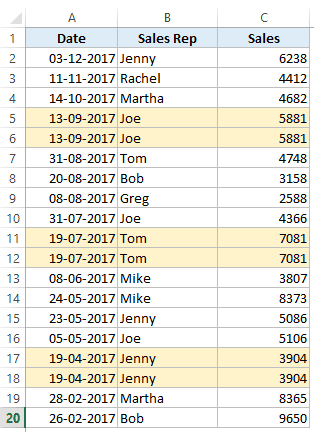
As you can see, there are duplicate records in this data set (highlighted in orange). These could be due to an error in data entry or result of data compilation.
In such a case, you can use Excel Advanced Filter tool to quickly get a list of all the unique records in a different location (so that your original data remains intact).
Here are the steps to get all the unique records:
This will instantly give you a list of all the unique records.

Caution: When you are using Advanced Filter to get the unique list, make sure you have also selected the header. If you don’t, it would consider the first cell as the header.
Example 2 – Using Criteria in Excel Advanced Filter
Getting unique records is one of the many things you can do with Excel advanced filter.
Its primary utility lies in its ability to allow using complex criteria for filtering data.
Here is what I mean by complex criteria. Suppose you have a dataset as shown below and you want to quickly get all the records where the sales are greater than 5000 and the region is the US.
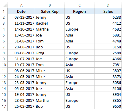
Here is how you can use Excel Advanced Filter to filter the records based on the specified criteria:
This would instantly give you all the records where the region is the US and the sales are more than 5000.

The above example is a case where the filtering is done based on two criteria (US and sales greater than 5000).
Excel Advanced filter allows you to create many different combinations of criteria.
Here are some examples of how you can construct these filters.
Using the AND Criteria
When you want to use AND criteria, you need to specify it below the header.
For example:
Using the OR Criteria
When you want to use OR criteria, you need to specify the criteria in the same column.
For example:
By now, you must have realized that when we have the criteria in the same row, it is an AND criteria, and when we have it in different rows, it is an OR criteria.
Example 3 – Using WILDCARD Characters in Advanced Filter in Excel
Excel Advanced Filter also allows the usage of wildcard characters while constructing the criteria.
There are three wildcard characters in Excel:
- * (asterisk) – It represents any number of characters. For example, ex* could mean excel, excels, example, expert, etc.
- ? (question mark) – It represents one single character. For example, Tr?mp could mean Trump or Tramp.
- ~ (tilde) – It is used to identify a wildcard character (~, *, ?) in the text.
Now let’s see how we can use these wildcard characters to do some advanced filtering in Excel.
- To filter records where the sales rep name starts from J.

Note that * represent any number of characters. So any rep with the name starting with J would be filtered with these criteria.
Similarly, you can use the other two wildcard characters as well.
Note: In case you’re using Office 365, you should check out the FILTER function. It can do a lot of things that advanced filter can do with a simple formula.
NOTE:
- Remember, the headers in the criteria should be exactly the same as that in the data set.
- Advanced filtering cannot be undone when copied to other locations.
You May Also Like the Following Excel Tutorials:
- Dynamic Excel Filter – Extract Data as you Type.
- Filtering Cells with Bold Font Formatting.
- How to Filter Cells that have Duplicate Text Strings (Words) in it.
- How to Filter Data in a Pivot Table in Excel
- MS Guide for Advanced Filter in Excel.
- How to Compare Two Columns in Excel.
- Excel VBA Autofilter
- 20 Advanced Excel Functions and Formulas (for Excel Pros)
Содержание
- Advanced filter in Excel and examples of its features
- Autofilter and advanced filter in Excel
- How to make an advanced filter in Excel
- How to use the advanced filter in Excel
- Filter by using advanced criteria
- Overview of advanced filter criteria
- Sample data
- Comparison operators
- Using the equal sign to type text or a value
- Considering case-sensitivity
- Using pre-defined names
- Creating criteria by using a formula
- Multiple criteria, one column, any criteria true
- Multiple criteria, multiple columns, all criteria true
- Multiple criteria, multiple columns, any criteria true
- Multiple sets of criteria, one column in all sets
- Multiple sets of criteria, multiple columns in each set
- Wildcard criteria
Advanced filter in Excel and examples of its features
The information can be displayed in several parameters using the data filtering in Excel. For this purpose, two tools are intended: an auto filter and an advanced filter. They do not delete, but hide data that does not fit the condition. Autofilter performs simple operations. This tool has many more features.
Autofilter and advanced filter in Excel
There is a simple table, not formatted and not declared by the list. You can enable the automatic filter through the main menu.
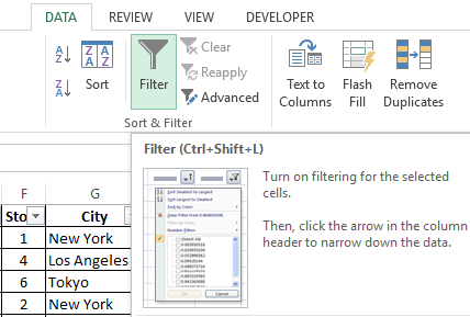
- Select any cell within the range with the mouse. Go to the «DATA» tab and press the «Filter» button.
- Next to the headings of the table, there are arrows that open the lists of the autofilter.
If you format the data range as a table or declare it as a list, the auto filter will be added immediately.
To use the auto-filter is a simple thing: you just need to select an entry with the desired value. For example, display the supplies to the store number. We put the tick in front of the corresponding filtering condition:
You can see the result immediately:
Peculiarities of the tool:
- AutoFilter works only in an unbroken range. Different tables on one sheet cannot be filtered, even if they have the same type of data.
- The tool treats the top line as column headers and these values are not included in the filter.
- It is acceptable to apply several filtering conditions at once. But each previous result can hide the records necessary for the next filter.
An extended filter has many more features:
- You can set as many conditions for filtering as you want.
- The criteria for selecting the data are visible.
- The user easily finds the unique values in a multi-line array with the help of the advanced filter.
How to make an advanced filter in Excel
A ready-made example is how to use the advanced filter in Excel:
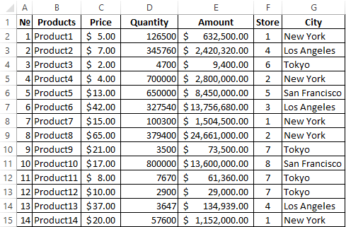
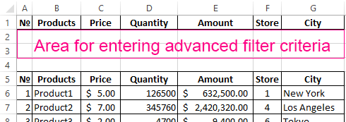
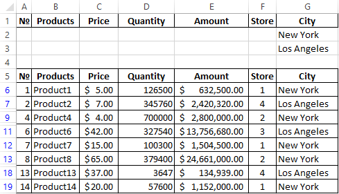
- Create a table with the selected conditions. To do this, copy the headers of the source list and insert it above. In the table with the criteria for filtering, we leave a sufficient number of rows plus an empty string separating from the original table.
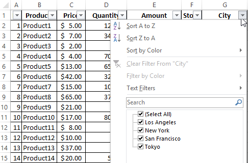
- We will set the filtration parameters for the selection of rows with the value «New York» (in the corresponding column of the table with the terms we enter name city – New York). Activate any cell in the source table. Go to the «DATA» tab — «Advanced».
- Fill in the filtering parameters. The initial range is the table with the original data. Links appear automatically, because one of the cells was active. A range of conditions is a condition label. Exit the Advanced menu by clicking OK.
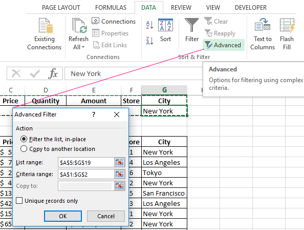
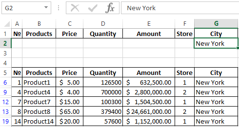
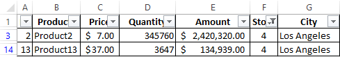
Only the lines containing the value «New York» remained in the source table. To cancel the filter, we should click the «Clear» button in the «Sort» section.
How to use the advanced filter in Excel
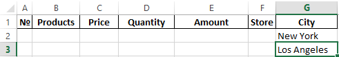
Consider using the advanced filter in Excel to select the lines containing the words «New York» or «Los Angeles». The conditions for filtering must be in the same column. It is each under another in our example.
Fill in the advanced filter menu:
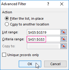
We get the table with the rows selected according to the specified criteria:
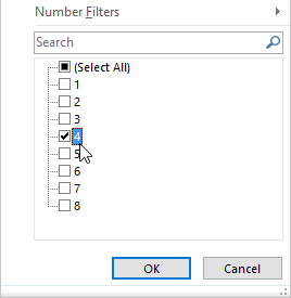
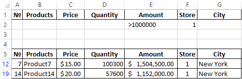
We will select the rows that contain the value «1» in the «Store» column, and the column value «> 1 000 000$». The criteria for filtering must be in the appropriate columns of the condition label in one line. Fill in the filtering parameters. Click OK.
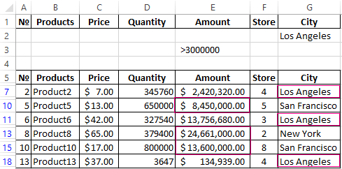
Leave in the table only those lines that contain the word «Los Angeles» in the column «City» or in the column «Amount» — the value «>3 000 000$». Since the selection criteria apply to different columns, we place them on different lines under the appropriate headings. Apply tool:
This tool can work with formulas, which allows the user to solve almost any task when selecting values from arrays.
- The result of the formula is a selection criterion.
- The recorded formula returns the result TRUE or FALSE.
- The initial range is indicated by absolute references, and the selection criterion (in the form of a formula) is using the relative references.
- If TRUE is returned, the string will be displayed after applying the filter. FALSE is not.
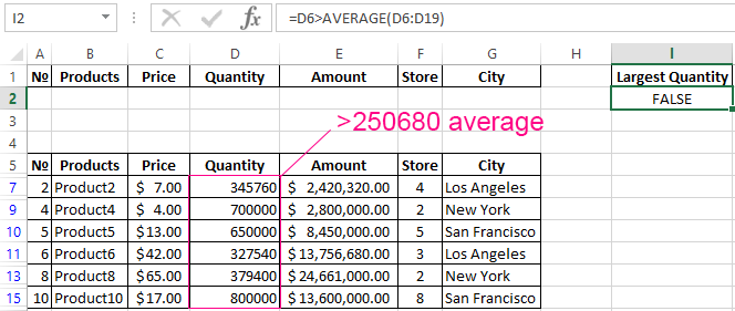
We display rows containing an amount above the average. For this purpose, aside from the table with the criteria (in cell I1), we will enter the name «Largest Quantity». Below is the formula. We use the AVERAGE function.
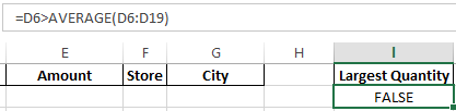
Select any cell in the original range and call the tool. As a criterion for the selection we indicate I1: I2.
Only those rows are left in the table, where the values in the «Quantity» column are above the average.
To leave only non-repeating lines in the table, in the «Advanced Filter» window put the birdie in front of «Unique records only».
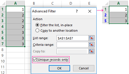
Click OK. Duplicate rows will be hidden. Only unique records remain on the sheet.
Источник
Filter by using advanced criteria
If the data you want to filter requires complex criteria (such as Type = «Produce» OR Salesperson = «Davolio»), you can use the Advanced Filter dialog box.
To open the Advanced Filter dialog box, click Data > Advanced.
Salesperson = «Davolio» OR Salesperson = «Buchanan»
Type = «Produce» AND Sales > 1000
Type = «Produce» OR Salesperson = «Buchanan»
(Sales > 6000 AND Sales 3000) OR
(Salesperson = «Buchanan» AND Sales > 1500)
Salesperson = a name with ‘u’ as the second letter
Overview of advanced filter criteria
The Advanced command works differently from the Filter command in several important ways.
It displays the Advanced Filter dialog box instead of the AutoFilter menu.
You type the advanced criteria in a separate criteria range on the worksheet and above the range of cells or table that you want to filter. Microsoft Office Excel uses the separate criteria range in the Advanced Filter dialog box as the source for the advanced criteria.
Sample data
The following sample data is used for all procedures in this article.
The data includes four blank rows above the list range that will be used as a criteria range (A1:C4) and a list range (A6:C10). The criteria range has column labels and includes at least one blank row between the criteria values and the list range.
To work with this data, select it in the following table, copy it, and then paste it in cell A1 of a new Excel worksheet.
Comparison operators
You can compare two values by using the following operators. When two values are compared by using these operators, the result is a logical value—either TRUE or FALSE.
> (greater than sign)
= (greater than or equal to sign)
Greater than or equal to
(not equal to sign)
Using the equal sign to type text or a value
Because the equal sign ( =) is used to indicate a formula when you type text or a value in a cell, Excel evaluates what you type; however, this may cause unexpected filter results. To indicate an equality comparison operator for either text or a value, type the criteria as a string expression in the appropriate cell in the criteria range:
Where entry is the text or value you want to find. For example:
What you type in the cell
What Excel evaluates and displays
Considering case-sensitivity
When filtering text data, Excel doesn’t distinguish between uppercase and lowercase characters. However, you can use a formula to perform a case-sensitive search. For an example, see the section Wildcard criteria.
Using pre-defined names
You can name a range Criteria, and the reference for the range will appear automatically in the Criteria range box. You can also define the name Database for the list range to be filtered and define the name Extract for the area where you want to paste the rows, and these ranges will appear automatically in the List range and Copy to boxes, respectively.
Creating criteria by using a formula
You can use a calculated value that is the result of a formula as your criterion. Remember the following important points:
The formula must evaluate to TRUE or FALSE.
Because you are using a formula, enter the formula as you normally would, and do not type the expression in the following way:
Do not use a column label for criteria labels; either keep the criteria labels blank or use a label that is not a column label in the list range (in the examples that follow, Calculated Average and Exact Match).
If you use a column label in the formula instead of a relative cell reference or a range name, Excel displays an error value such as #NAME? or #VALUE! in the cell that contains the criterion. You can ignore this error because it does not affect how the list range is filtered.
The formula that you use for criteria must use a relative reference to refer to the corresponding cell in the first row of data.
All other references in the formula must be absolute references.
Multiple criteria, one column, any criteria true
Boolean logic: (Salesperson = «Davolio» OR Salesperson = «Buchanan»)
Insert at least three blank rows above the list range that can be used as a criteria range. The criteria range must have column labels. Make sure that there is at least one blank row between the criteria values and the list range.
To find rows that meet multiple criteria for one column, type the criteria directly below each other in separate rows of the criteria range. Using the example, enter:
Click a cell in the list range. Using the example, click any cell in the range A6:C10.
On the Data tab, in the Sort & Filter group, click Advanced.
Do one of the following:
To filter the list range by hiding rows that don’t match your criteria, click Filter the list, in-place.
To filter the list range by copying rows that match your criteria to another area of the worksheet, click Copy to another location, click in the Copy to box, and then click the upper-left corner of the area where you want to paste the rows.
Tip When you copy filtered rows to another location, you can specify which columns to include in the copy operation. Before filtering, copy the column labels for the columns that you want to the first row of the area where you plan to paste the filtered rows. When you filter, enter a reference to the copied column labels in the Copy to box. The copied rows will then include only the columns for which you copied the labels.
In the Criteria range box, enter the reference for the criteria range, including the criteria labels. Using the example, enter $A$1:$C$3.
To move the Advanced Filter dialog box out of the way temporarily while you select the criteria range, click Collapse Dialog  .
.
Using the example, the filtered result for the list range is:
Multiple criteria, multiple columns, all criteria true
Boolean logic: (Type = «Produce» AND Sales > 1000)
Insert at least three blank rows above the list range that can be used as a criteria range. The criteria range must have column labels. Make sure that there is at least one blank row between the criteria values and the list range.
To find rows that meet multiple criteria in multiple columns, type all the criteria in the same row of the criteria range. Using the example, enter:
Click a cell in the list range. Using the example, click any cell in the range A6:C10.
On the Data tab, in the Sort & Filter group, click Advanced.
Do one of the following:
To filter the list range by hiding rows that don’t match your criteria, click Filter the list, in-place.
To filter the list range by copying rows that match your criteria to another area of the worksheet, click Copy to another location, click in the Copy to box, and then click the upper-left corner of the area where you want to paste the rows.
Tip When you copy filtered rows to another location, you can specify which columns to include in the copy operation. Before filtering, copy the column labels for the columns that you want to the first row of the area where you plan to paste the filtered rows. When you filter, enter a reference to the copied column labels in the Copy to box. The copied rows will then include only the columns for which you copied the labels.
In the Criteria range box, enter the reference for the criteria range, including the criteria labels. Using the example, enter $A$1:$C$2.
To move the Advanced Filter dialog box out of the way temporarily while you select the criteria range, click Collapse Dialog .
Using the example, the filtered result for the list range is:
Multiple criteria, multiple columns, any criteria true
Boolean logic: (Type = «Produce» OR Salesperson = «Buchanan»)
Insert at least three blank rows above the list range that can be used as a criteria range. The criteria range must have column labels. Make sure that there is at least one blank row between the criteria values and the list range.
To find rows that meet multiple criteria in multiple columns where any criteria can be true, type the criteria in the different columns and rows of the criteria range. Using the example, enter:
Click a cell in the list range. Using the example, click any cell in the list range A6:C10.
On the Data tab, in the Sort & Filter group, click Advanced.
Do one of the following:
To filter the list range by hiding rows that don’t match your criteria, click Filter the list, in-place.
To filter the list range by copying rows that match your criteria to another area of the worksheet, click Copy to another location, click in the Copy to box, and then click the upper-left corner of the area where you want to paste the rows.
Tip: When you copy filtered rows to another location, you can specify which columns to include in the copy operation. Before filtering, copy the column labels for the columns that you want to the first row of the area where you plan to paste the filtered rows. When you filter, enter a reference to the copied column labels in the Copy to box. The copied rows will then include only the columns for which you copied the labels.
In the Criteria range box, enter the reference for the criteria range, including the criteria labels. Using the example, enter $A$1:$B$3.
To move the Advanced Filter dialog box out of the way temporarily while you select the criteria range, click Collapse Dialog .
Using the example, the filtered result for the list range is:
Multiple sets of criteria, one column in all sets
Boolean logic: ( (Sales > 6000 AND Sales
To find rows that meet multiple sets of criteria where each set includes criteria for one column, include multiple columns with the same column heading. Using the example, enter:
Click a cell in the list range. Using the example, click any cell in the list range A6:C10.
On the Data tab, in the Sort & Filter group, click Advanced.
Do one of the following:
To filter the list range by hiding rows that don’t match your criteria, click Filter the list, in-place.
To filter the list range by copying rows that match your criteria to another area of the worksheet, click Copy to another location, click in the Copy to box, and then click the upper-left corner of the area where you want to paste the rows.
Tip: When you copy filtered rows to another location, you can specify which columns to include in the copy operation. Before filtering, copy the column labels for the columns that you want to the first row of the area where you plan to paste the filtered rows. When you filter, enter a reference to the copied column labels in the Copy to box. The copied rows will then include only the columns for which you copied the labels.
In the Criteria range box, enter the reference for the criteria range, including the criteria labels. Using the example, enter $A$1:$D$3.
To move the Advanced Filter dialog box out of the way temporarily while you select the criteria range, click Collapse Dialog .
Using the example, the filtered result for the list range is:
Multiple sets of criteria, multiple columns in each set
Boolean logic: ( (Salesperson = «Davolio» AND Sales >3000) OR (Salesperson = «Buchanan» AND Sales > 1500) )
Insert at least three blank rows above the list range that can be used as a criteria range. The criteria range must have column labels. Make sure that there is at least one blank row between the criteria values and the list range.
To find rows that meet multiple sets of criteria, where each set includes criteria for multiple columns, type each set of criteria in separate columns and rows. Using the example, enter:
Click a cell in the list range. Using the example, click any cell in the list range A6:C10.
On the Data tab, in the Sort & Filter group, click Advanced.
Do one of the following:
To filter the list range by hiding rows that don’t match your criteria, click Filter the list, in-place.
To filter the list range by copying rows that match your criteria to another area of the worksheet, click Copy to another location, click in the Copy to box, and then click the upper-left corner of the area where you want to paste the rows.
Tip When you copy filtered rows to another location, you can specify which columns to include in the copy operation. Before filtering, copy the column labels for the columns that you want to the first row of the area where you plan to paste the filtered rows. When you filter, enter a reference to the copied column labels in the Copy to box. The copied rows will then include only the columns for which you copied the labels.
In the Criteria range box, enter the reference for the criteria range, including the criteria labels. Using the example, enter $A$1:$C$3.To move the Advanced Filter dialog box out of the way temporarily while you select the criteria range, click Collapse Dialog .
Using the example, the filtered result for the list range would be:
Wildcard criteria
Boolean logic: Salesperson = a name with ‘u’ as the second letter
To find text values that share some characters but not others, do one or more of the following:
Type one or more characters without an equal sign ( =) to find rows with a text value in a column that begin with those characters. For example, if you type the text Dav as a criterion, Excel finds «Davolio,» «David,» and «Davis.»
Use a wildcard character.
Any single character
For example, sm?th finds «smith» and «smyth»
Any number of characters
For example, *east finds «Northeast» and «Southeast»
(tilde) followed by ?, *, or
A question mark, asterisk, or tilde
For example, fy91
Insert at least three blank rows above the list range that can be used as a criteria range. The criteria range must have column labels. Make sure that there is at least one blank row between the criteria values and the list range.
In the rows below the column labels, type the criteria that you want to match. Using the example, enter:
Click a cell in the list range. Using the example, click any cell in the list range A6:C10.
On the Data tab, in the Sort & Filter group, click Advanced.
Do one of the following:
To filter the list range by hiding rows that don’t match your criteria, click Filter the list, in-place
To filter the list range by copying rows that match your criteria to another area of the worksheet, click Copy to another location, click in the Copy to box, and then click the upper-left corner of the area where you want to paste the rows.
Tip: When you copy filtered rows to another location, you can specify which columns to include in the copy operation. Before filtering, copy the column labels for the columns that you want to the first row of the area where you plan to paste the filtered rows. When you filter, enter a reference to the copied column labels in the Copy to box. The copied rows will then include only the columns for which you copied the labels.
In the Criteria range box, enter the reference for the criteria range, including the criteria labels. Using the example, enter $A$1:$B$3.
To move the Advanced Filter dialog box out of the way temporarily while you select the criteria range, click Collapse Dialog .
Using the example, the filtered result for the list range is:
Источник

on
July 21, 2010, 7:00 AM PDT
How to use And and Or operators with Excel’s Advanced Filter
Use implicit And and Or operators with Excel’s Advanced Filter feature to create complex, but powerful, filtering combos.
Editor’s Note: This article was originally published in July 2010 and the video tutorial for this article published Dec. 2018; while this program might look a little different, the steps shown in this tutorial are the same.
Viewing subsets of data is a routine task for many Excel users. An AutoFilter lets you limit the data displayed, but it’s limited as it depends on the actual data. Excel’s Advanced Filter feature requires a bit of setup, but is more flexible and powerful than an AutoFilter. Not only can you use an expression to match records, you can combine expressions using the And and Or operators – now, that’s power!
This blog post is also available as a TechRepublic Photo Gallery.
Excel’s Advanced Filter feature requires three elements:
- Data
- A criteria range, where you specify criteria as an expression.
- An extract range, where Excel displays the data that satisfies the criteria.
LEARN MORE: Office 365 Consumer pricing and features
A simple AutoFilter
Before we get into a more advanced example, let’s look at a simple AutoFilter example using a partial set of data from the Products table from Northwind (the database that comes with Access). To apply an AutoFilter, you select the column headings in A1:F1 and choose AutoFilter from the Data menu. In Excel 2007 and 2010, click the Data menu and then click Filter in the Sort & Filter group. Excel will display a dropdown arrow for each column in the selection. Using this feature, you can perform simple filtering tasks, such as which products have no units on order. It’s quick and easy, but sometimes inadequate. (To remove a filter, simply choose All from the same list.)
An Advanced Filter and And
Now, suppose you wanted to know which products with a price of $20 or more have 10 or less units currently in stock. This filtering task has two requirements – two criteria – and you want to satisfy them both. In other words, the product must be $20 or more and have 10 or fewer units in stock. An AutoFilter just can’t do that, so let’s try an Advanced Filter.
The criteria range, in this case, requires only two columns: Unit Price and Units In Stock. You could copy just those column headings to an out of the way place. I recommend copying all of the headers – you might need them for another filter.
SEE: Crash Course: Microsoft Excel – Beginner (Tech Pro Research)
Next, you need to state your filtering requirements in terms Excel can understand, using an expression. In this case, both expressions are simple comparisons:
Unit Price: >=20
Units In Stock: <=10
As you can see, the criteria range is above the actual data. This placement is efficient and easily accessible. Both expressions are in the same row – row 2. By placing both expressions in the same row, Excel knows to apply an implicit And operator to combine the expressions.
All that’s left now is to apply the filter as follows:
- Click any cell in the data range.
- Click the Data menu, and then click Filter | Advanced Filter. In Excel 2007 and 2010, click the Data tab and then click Advanced Filter in the Sort & Filter group.
- Retain the default setting, Filter the List In-Place.
- Excel automatically fills in the List Range, correctly in this case.
- Specify the Criteria range, A1:F2. You only need to identify the column headings and the criteria row or rows.

- Click OK.

Eight products have a price of $20 or more and have 10 or fewer units in stock. To remove the filter, click the Data menu, then click Filter | Show All.
An Advanced Filter and Or
To specify an implicit Or operator, you must place the expressions in separate rows. The criteria shown below will find products with a price of $20 or more or products with 10 or fewer products in stock.
After adjusting the criteria range by moving one of the expressions down a row, apply the new filter as follows:
- Click any cell in the data range.
- Click the Data menu, and then click Filter | Advanced Filter. In Excel 2007 and 2010, click the Data tab and then click Advanced Filter.
- Retain the Filter the List In Place setting, the default.
- Excel automatically fills in the List Range, correctly in this case.
- Specify the Criteria range–that’s A1:F3. Notice that this time, the range includes row 3.

- Click OK. Many records meet one or the other criteria.


You can use an Advanced Filter with just one expression, but using implicit And and Or operators opens the door for some very complex but powerful filters. Just be careful that the expressions and their placement make sense, in terms of applying the And and Or operators.
Affiliate disclosure: TechRepublic may earn a commission from the products and services featured on this page.
Also See
-
How to add a drop-down list to an Excel cell
(TechRepublic) -
Build your Excel skills with these 10 power tips (free PDF)
(TechRepublic) -
You’ve been using Excel wrong all along (and that’s OK)
(ZDNet) -
A cheatsheet of Excel shortcuts that make inserting data faster
(TechRepublic) -
Six clicks: Excel power tips to make you an instant expert
(ZDNet) -
10 advanced formatting tricks for Excel users
(TechRepublic)
-
Microsoft
-
Software
Author: Oscar Cronquist Article last updated on March 31, 2022
1. How to filter using OR logic between columns
The built-in filter feature in Excel is a powerful tool, however, it won’t allow you to filter with OR logic between columns.
This is where the Advanced Filter comes into the picture. It lets you do that and I will show you how now.
Copy your table headers and paste them somewhere on your worksheet.
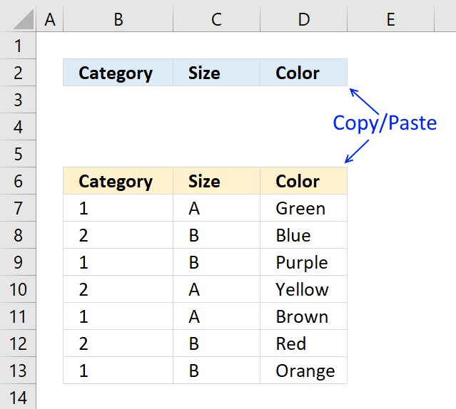
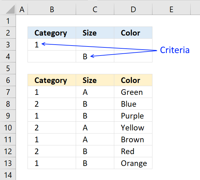
Type the criteria you want to use right below the new headers, each below the header you want to filter, see picture below.
Make sure the condition is the only one on each row.
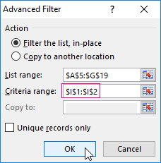
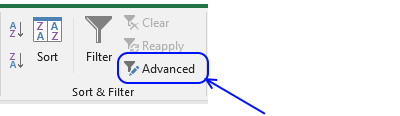
Now it is time to start the Advanced Filter. Go to tab «Data» on the ribbon and press with left mouse button on «Advanced Filter» button.
The «Advanced Filter» settings window appears.
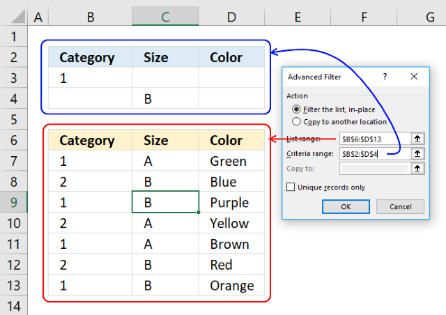
Press with mouse on «List range:» field and select cell range B6:D13 (your data you want to filter).
Press with mouse on «Criteria range:» field and select cell range B2:D4 (your criteria you want to use).
Press with left mouse button on OK button.
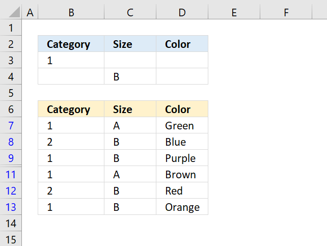
The blue rows to the left show you that you have applied a filter to your data.
To clear the filter simply press with left mouse button on the clear button on the ribbon tab «Data».
![]()
Get Excel *.xlsx file
How to filter with OR logic between columns.xlsx
Back to top
2. Advanced custom date filter
Question: How do I filter the last xx years or xx months in Excel?
How do I exclude the current month when using the year to date filter in Excel?
Answer: Use advanced filter with criteria ranges. I have calculated the exact dates needed to create the criteria ranges.
I will go through the exact steps on how to accomplish the date filter.
The picture below shows the calculation of the dates, the criteria ranges and the list to filter.

How to create a criteria range
- Copy the header of the list to a new location, see cell A16:C16 in the above picture.
- Type the criteria, see A17:B17 in the above picture.
- Formula in A17:
=»<=2009-07-31″ + ENTER
Formula in B17:
=»>=2009-01-01″ + ENTER
How to filter a list using a criteria range
- Press with left mouse button on «Data» in the ribbon
- Press with left mouse button on Advanced

- Select List range: A27:C64

- Select the criteria range A16:C17
- Press with left mouse button on OK!


The new filtered list.

Repeat the above steps to filter the last xx years or xx months using the criteria ranges.
Get excel example file.
filter-a-list-of-dates.xlsx
(Excel 2007 Workbook *.xlsx)
Back to top
Latest updated articles.
More than 300 Excel functions with detailed information including syntax, arguments, return values, and examples for most of the functions used in Excel formulas.
More than 1300 formulas organized in subcategories.
Excel Tables simplifies your work with data, adding or removing data, filtering, totals, sorting, enhance readability using cell formatting, cell references, formulas, and more.
Allows you to filter data based on selected value , a given text, or other criteria. It also lets you filter existing data or move filtered values to a new location.
Lets you control what a user can type into a cell. It allows you to specifiy conditions and show a custom message if entered data is not valid.
Lets the user work more efficiently by showing a list that the user can select a value from. This lets you control what is shown in the list and is faster than typing into a cell.
Lets you name one or more cells, this makes it easier to find cells using the Name box, read and understand formulas containing names instead of cell references.
The Excel Solver is a free add-in that uses objective cells, constraints based on formulas on a worksheet to perform what-if analysis and other decision problems like permutations and combinations.
An Excel feature that lets you visualize data in a graph.
Format cells or cell values based a condition or criteria, there a multiple built-in Conditional Formatting tools you can use or use a custom-made conditional formatting formula.
Lets you quickly summarize vast amounts of data in a very user-friendly way. This powerful Excel feature lets you then analyze, organize and categorize important data efficiently.
VBA stands for Visual Basic for Applications and is a computer programming language developed by Microsoft, it allows you to automate time-consuming tasks and create custom functions.
A program or subroutine built in VBA that anyone can create. Use the macro-recorder to quickly create your own VBA macros.
UDF stands for User Defined Functions and is custom built functions anyone can create.
A list of all published articles.