
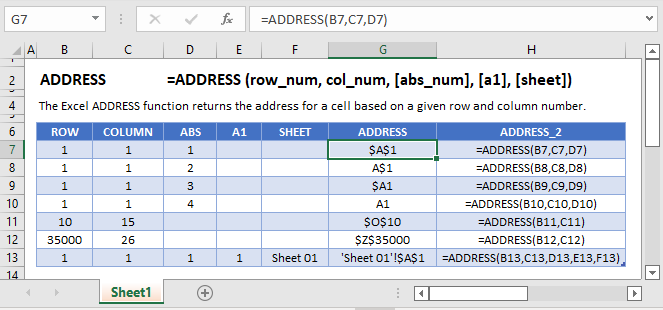
The Excel ADDRESS function returns a cell reference as a string, based on a row and column number
Example: Excel ADDRESS Function

METHOD 1. Excel ADDRESS function using hardcoded values
EXCEL
|
Result in cell G5 ($D$3) — returns the assigned cell reference that comprises only the required ADDRESS arguments (row number and column number)) as a string. |
|
Result in cell G6 ($D$3) — returns the assigned cell reference that comprises the required ADDRESS arguments (row number and column number) and an abs number (Absolute row and column) as a string. |
|
Result in cell G7 (D$3) — returns the assigned cell reference that comprises the required ADDRESS arguments (row number and column number) and an abs number (Absolute row and Relative column) as a string. |
|
Result in cell G8 ($D3) — returns the assigned cell reference that comprises the required ADDRESS arguments (row number and column number) and an abs number (Relative row and Absolute column) as a string. |
|
Result in cell G9 (D3) — returns the assigned cell reference that comprises the required ADDRESS arguments (row number and column number) and an abs number (Relative row and column) as a string. |
|
Result in cell G10 ($D$3) — returns the assigned cell reference that comprises the required ADDRESS arguments (row number and column number), abs number (Absolute row and column) and A1 reference style as a string. |
|
Result in cell G11 ($D$3) — returns the assigned cell reference that comprises the required ADDRESS arguments (row number and column number) and A1 reference style as a string. |
|
Result in cell G12 (R3C3) — returns the assigned cell reference that comprises the required ADDRESS arguments (row number and column number), abs number (Absolute row and column) and R1C1 reference style as a string. |
|
=ADDRESS(3,4,1,TRUE,»Sheet1″) |
Result in cell G13 (Sheet1!$D$3) — returns the assigned cell reference that comprises the required ADDRESS arguments (row number and column number), abs number (Absolute row and column), A1 reference style and reference a sheet name as a string. |
METHOD 2. Excel ADDRESS function using links
EXCEL
|
Result in cell G5 ($D$3) — returns the assigned cell reference that comprises only the required ADDRESS arguments (row number and column number)) as a string. |
|
Result in cell G6 ($D$3) — returns the assigned cell reference that comprises the required ADDRESS arguments (row number and column number) and an abs number (Absolute row and column) as a string. |
|
Result in cell G7 (D$3) — returns the assigned cell reference that comprises the required ADDRESS arguments (row number and column number) and an abs number (Absolute row and Relative column) as a string. |
|
Result in cell G8 ($D3) — returns the assigned cell reference that comprises the required ADDRESS arguments (row number and column number) and an abs number (Relative row and Absolute column) as a string. |
|
Result in cell G9 (D3) — returns the assigned cell reference that comprises the required ADDRESS arguments (row number and column number) and an abs number (Relative row and column) as a string. |
|
Result in cell G10 ($D$3) — returns the assigned cell reference that comprises the required ADDRESS arguments (row number and column number), abs number (Absolute row and column) and A1 reference style as a string. |
|
Result in cell G11 ($D$3) — returns the assigned cell reference that comprises the required ADDRESS arguments (row number and column number) and A1 reference style as a string. |
|
Result in cell G12 (R3C3) — returns the assigned cell reference that comprises the required ADDRESS arguments (row number and column number), abs number (Absolute row and column) and R1C1 reference style as a string. |
|
=ADDRESS(B13,C13,D13,E13,F13) |
Result in cell G13 (Sheet1!$D$3) — returns the assigned cell reference that comprises the required ADDRESS arguments (row number and column number), abs number (Absolute row and column), A1 reference style and reference a sheet name as a string. |
METHOD 3. Excel ADDRESS function using the Excel built-in function library with hardcoded value
EXCEL
Formulas tab > Function Library group > Lookup & Reference > ADDRESS > populate the input boxes
| = ADDRESS(3,4,1,TRUE,»Sheet1″) Note: in this example we are populating all of the input boxes associated with the ADDRESS function arguments, however, you are only required to populate the required arguments (Row_num and Column_num). You can omit the optional arguments and Excel will apply its default value against each of them. |
 |
METHOD 4. Excel ADDRESS function using the Excel built-in function library with links
EXCEL
Formulas tab > Function Library group > Lookup & Reference > ADDRESS > populate the input boxes
| = ADDRESS(B13,C13,D13,E13,F13) Note: in this example we are populating all of the input boxes associated with the ADDRESS Function arguments with links, however, you are only required to populate the required arguments (Row_num and Column_num). You can omit the optional arguments and Excel will apply the default value against each of them. |
 |
METHOD 1. Excel ADDRESS function using VBA with hardcoded values
VBA
Sub Excel_ADDRESS_Function_Using_Hardcoded_Values()
‘declare a variable
Dim ws As Worksheet
Set ws = Worksheets(«ADDRESS»)
‘apply the Excel ADDRESS function
ws.Range(«G5») = ws.Cells(3, 4).Address()
ws.Range(«G6») = ws.Cells(3, 4).Address(RowAbsolute:=True)
ws.Range(«G7») = ws.Cells(3, 4).Address(ColumnAbsolute:=False)
ws.Range(«G8») = ws.Cells(3, 4).Address(RowAbsolute:=False)
ws.Range(«G9») = ws.Cells(3, 4).Address(RowAbsolute:=False, ColumnAbsolute:=False)
ws.Range(«G10») = ws.Cells(3, 4).Address(RowAbsolute:=True, ReferenceStyle:=xlA1)
ws.Range(«G11») = ws.Cells(3, 4).Address(ReferenceStyle:=xlA1)
ws.Range(«G12») = ws.Cells(3, 4).Address(RowAbsolute:=True, ReferenceStyle:=xlR1C1)
ws.Range(«G13») = «‘» & ThisWorkbook.Worksheets(«Sheet1»).Cells(1, 1).Parent.Name & «‘!» & ws.Cells(3, 4).Address(RowAbsolute:=True)
End Sub
OBJECTS
Range: The Range object is a representation of a single cell or a range of cells in a worksheet.
Worksheets: The Worksheets object represents all of the worksheets in a workbook, excluding chart sheets.
PREREQUISITES
Worksheet Name: Have a worksheet named ADDRESS.
ADJUSTABLE PARAMETERS
Output Range: Select the output range by changing the cell references («G5»), («G6»), («G7»), («G8»), («G9»), («G10»), («G11»), («G12») and («G13») in the VBA code to any cell in the worksheet, that doesn’t conflict with the formula.
METHOD 2. Excel ADDRESS function using VBA with links
VBA
Sub Excel_ADDRESS_Function_Using_Links()
‘declare a variable
Dim ws As Worksheet
Set ws = Worksheets(«ADDRESS»)
‘apply the Excel ADDRESS function
ws.Range(«G5») = ws.Cells(Range(«B5»), Range(«C5»)).Address()
ws.Range(«G6») = ws.Cells(Range(«B6»), Range(«C6»)).Address(RowAbsolute:=True)
ws.Range(«G7») = ws.Cells(Range(«B7»), Range(«C7»)).Address(ColumnAbsolute:=False)
ws.Range(«G8») = ws.Cells(Range(«B8»), Range(«C8»)).Address(RowAbsolute:=False)
ws.Range(«G9») = ws.Cells(Range(«B9»), Range(«C9»)).Address(RowAbsolute:=False, ColumnAbsolute:=False)
ws.Range(«G10») = ws.Cells(Range(«B10»), Range(«C10»)).Address(RowAbsolute:=True, ReferenceStyle:=xlA1)
ws.Range(«G11») = ws.Cells(Range(«B11»), Range(«C11»)).Address(ReferenceStyle:=xlA1)
ws.Range(«G12») = ws.Cells(Range(«B12»), Range(«C12»)).Address(RowAbsolute:=True, ReferenceStyle:=xlR1C1)
ws.Range(«G13») = «‘» & ThisWorkbook.Worksheets(«Sheet1»).Cells(1, 1).Parent.Name & «‘!» & ws.Cells(Range(«B13»), Range(«C13»)).Address(RowAbsolute:=True)
End Sub
OBJECTS
Range: The Range object is a representation of a single cell or a range of cells in a worksheet.
Worksheets: The Worksheets object represents all of the worksheets in a workbook, excluding chart sheets.
PREREQUISITES
Worksheet Name: Have a worksheet named ADDRESS.
ADJUSTABLE PARAMETERS
Output Range: Select the output range by changing the cell references («G5»), («G6»), («G7»), («G8»), («G9»), («G10»), («G11»), («G12») and («G13») in the VBA code to any cell in the worksheet, that doesn’t conflict with the formula.
METHOD 3. Excel ADDRESS function using VBA with ranges
VBA
Sub Excel_ADDRESS_Function_Using_Ranges()
‘declare a variable
Dim ws As Worksheet
Set ws = Worksheets(«ADDRESS»)
‘apply the Excel ADDRESS function
ws.Range(«G5») = ws.Range(«D3»).Address()
ws.Range(«G6») = ws.Range(«D3»).Address(RowAbsolute:=True)
ws.Range(«G7») = ws.Range(«D3»).Address(ColumnAbsolute:=False)
ws.Range(«G8») = ws.Range(«D3»).Address(RowAbsolute:=False)
ws.Range(«G9») = ws.Range(«D3»).Address(RowAbsolute:=False, ColumnAbsolute:=False)
ws.Range(«G10») = ws.Range(«D3»).Address(RowAbsolute:=True, ReferenceStyle:=xlA1)
ws.Range(«G11») = ws.Range(«D3»).Address(ReferenceStyle:=xlA1)
ws.Range(«G12») = ws.Range(«D3»).Address(RowAbsolute:=True, ReferenceStyle:=xlR1C1)
ws.Range(«G13») = «‘» & ThisWorkbook.Worksheets(«Sheet1»).Cells(1, 1).Parent.Name & «‘!» & ws.Range(«D3»).Address(RowAbsolute:=True)
End Sub
OBJECTS
Range: The Range object is a representation of a single cell or a range of cells in a worksheet.
Worksheets: The Worksheets object represents all of the worksheets in a workbook, excluding chart sheets.
PREREQUISITES
Worksheet Name: Have a worksheet named ADDRESS.
ADJUSTABLE PARAMETERS
Output Range: Select the output range by changing the cell references («G5»), («G6»), («G7»), («G8»), («G9»), («G10»), («G11»), («G12») and («G13») in the VBA code to any cell in the worksheet, that doesn’t conflict with the formula.
Usage of the Excel ADDRESS function and formula syntax
EXPLANATION
DESCRIPTION
The Excel ADDRESS function returns a cell reference as a string, based on a row and column number.
SYNTAX
=ADDRESS(row_num, column_num, [abs_num],[a1],[sheet_text])
ARGUMENT(S)
row_num: (Required) Row number to use in the reference.
column_num: (Required) Column number to use in the reference.
abs_num: (Optional) Type of address reference to use. This can be any of the following values:
| Value | Explanation | Example |
|---|---|---|
| 1 | Absolute row and column | $A$1 |
| 2 | Absolute row and Relative column | A$1 |
| 3 | Relative row and Absolute column | $A1 |
| 4 | Relative row and column | A1 |
Note: If the abs_num argument is omitted, the default value is 1 (Absolute row and column).
a1: (Optional) Specifies what type of reference style to use. This can be any of the following:
| Value | Explanation | Example |
|---|---|---|
| TRUE | A1 reference style | A1, A2, B2 |
| FALSE | R1C1 reference style | R1C1, R2C1, R2C2 |
Note: If the a1 argument is omitted, the default value is TRUE (A1 reference style).
sheet_text: (Optional) Specifies the name of the worksheet to be used. You will need to insert the name between the quotation marks («Name»).
Note: If the sheet_text argument is omitted, no sheet name will appear.
In this example the goal is to return the full address of a range or named range as text. The purpose of this formula is informational, not functional. It provides a way to inspect the current range for a named range, an Excel Table, or even the result of a formula. The core of the solutions explained below is the ADDRESS function, which returns a cell address based on a given row and column. The formula gets somewhat complicated because we need to use ADDRESS twice, and because there is a lot of busy work in collecting the coordinates we need to provide to ADDRESS. See below for a more elegant formula that takes advantage of the LET function and the TAKE function in Excel 365. This version can also report the range returned by another function (like OFFSET).
Note: the CELL function is another way to get the address for a cell. However, CELL does not provide a way to choose a relative or absolute format like the ADDRESS function does. In addition, CELL is a volatile function and can cause performance problems in large or complex worksheets. For those reasons, I have avoided it in this example.
Background
The links below provide more details about Excel Tables and named ranges:
- How to create an Excel Table (video)
- How to create a named range (video)
- How to create a dynamic named range with a table (video)
Demo
The animation below shows how the formula responds when a Table named «data» is resized. In the worksheet, DA stands for Dynamic Array version of Excel and Legacy stands for older versions of Excel. See below for more information about the dynamic array version.

The basic idea
The basic idea of this formula is to get the coordinates of the first (upper left) cell in a range and the last (lower right) cell in a range, then use these coordinates to create cell references, then join the references together with concatenation. The formula itself looks complicated and scary:
=ADDRESS(@ROW(data),@COLUMN(data),4)&":"&ADDRESS(@ROW(data)+ROWS(data)-1,@COLUMN(data)+COLUMNS(data)-1,4)However, most of what you see is the «busy work» of collecting the coordinates with the ROW, ROWS, COLUMN, and COLUMNS functions. Once that work is done, the formula simplifies to this:
=ADDRESS(5,2,4)&":"&ADDRESS(16,4,4)The ADDRESS function then creates a reference to the first and last cell in the range, and the two references are joined together. That’s it. The rest of the problem is the details of collecting the coordinates needed by the ADDRESS function.
ROW and COLUMN functions
The ROW and COLUMN functions simply return coordinates. For example, if we give ROW and COLUMN cell B5 as a reference, we get back coordinate numbers:
=ROW(B5) // returns 5
=COLUMN(B5) // returns 2
Notice that COLUMN returns a number, not a letter: column A, is 1, column B is 2, column C is 3, etc.
ROWS and COLUMNS functions
The ROWS and COLUMNS functions return counts. For example, if we give ROWS and COLUMNS the range B5:D16, we get back the number of rows and the number of columns in the range:
=ROWS(B5:D16) // returns 12
=COLUMNS(B5:D16) // returns 3
ADDRESS function
The ADDRESS function returns the address for a cell based on a given row and column number as text. For example:
=ADDRESS(1,1) // returns "$A$1"
=ADDRESS(5,2) // returns "$B$5"
Note that ADDRESS returns an address as an absolute reference by default. However, by providing 4 for the optional argument abs_num, ADDRESS will return a relative reference:
=ADDRESS(1,1,4) // returns "A1"
=ADDRESS(5,2,4) // returns "B5"
In this problem, we need to build up an address for a range in two parts (1) a reference to the first cell in the range and (2) a reference to the last cell in a range. To get the address for the first cell in the range, we use this formula:
=ADDRESS(@ROW(data),@COLUMN(data))
Note: data is the named range B5:E16.
As mentioned above, the ROW function and the COLUMN function return coordinates: ROW returns a row number, and COLUMN returns a column number. In this case however, we are giving ROW and COLUMN the range data, not a single cell. As a result, we get back an array of numbers:
=ROW(data) // returns {5;6;7;8;9;10;11;12;13;14;15;16}
=COLUMN(data) // returns {2,3,4,5}
In other words, ROW returns all row numbers for data (B5:D15), and COLUMN returns all column numbers for data. This is where the formula gets a bit complicated due to Excel version differences.
Although ROW and COLUMN return multiple results, older versions of Excel will automatically limit the results to the first value only. This works fine for the problem at hand, because we only want the first value. However, in the dynamic version of Excel, multiple results are not automatically limited, because formulas can spill results onto the worksheet. We don’t want this behavior in this case, so we use the implicit intersection operator (@) to limit the output from ROW and COLUMN to one value only:
=@ROW(data) // returns 5
=@COLUMN(data) // returns 2
In effect, this mimics the behavior in Legacy Excel where formulas that return more than one result display one result only. Note that the implicit intersection operator (@) is not required in Legacy Excel. In fact, if you try to add the @ in an older version of Excel, Excel will simply remove it. However, it is required in the current version of Excel.
Returning to the formula, ROW and COLUMN return their results directly to ADDRESS as the row_num and column_num arguments. With abs_num provided as 4 (relative), ADDRESS returns the text «B5».
=ADDRESS(5,2,4) // returns "B5"
To get the last cell in the range, we use the ADDRESS function again like this:
ADDRESS(@ROW(data)+ROWS(data)-1,@COLUMN(data)+COLUMNS(data)-1,4)
Essentially, we follow the same idea as above, using ROW and COLUMN to get the last row and last column of the range. However we also calculate the total number of rows with the ROWS function and the total number of columns with the COLUMNS function:
=ROWS(data) // returns 12
=COLUMNS(data) // returns 4
Then we do some simple math to calculate the row and column number of the last cell. We add the row count to the starting row, and add the column count to the starting column, then subtract 1 to get the correct coordinates for the last cell:
=ADDRESS(@ROW(data)+ROWS(data)-1,@COLUMN(data)+COLUMNS(data)-1,4)
=ADDRESS(5+12-1,2+4-1,4)
=ADDRESS(16,5,4)
="E16"
With abs_num set to 4. ADDRESS returns «E16», the address of the last cell in data as text. At this point, we have the address for the first cell and the address for the last cell. The only thing left to do is concatenate them together separated by a colon:
="B5"&":"&"E16"
="B5:E16"
More elegant formula
Although the formula above works fine, it is cumbersome and redundant. New array functions in Excel make it possible to solve the problem with a more elegant formula like this:
=LET(
first,TAKE(rng,1,1),
last,TAKE(rng,-1,-1),
ADDRESS(ROW(first),COLUMN(first),4)&":"&
ADDRESS(ROW(last),COLUMN(last),4)
)
Where rng is the generic placeholder for a named range or Excel Table. In this formula, the LET function is used to assign values to two variables: first and last. First represents the first cell in the range and last represents the last cell in the range. These values are assigned with the TAKE function like this:
first,TAKE(rng,1,1), // first cell (B5)
last,TAKE(rng,-1,-1), // last cell (E16)
The TAKE function returns a subset of a given array or range. The size of the array returned is determined by separate rows and columns arguments. When positive numbers are provided for rows or columns, TAKE returns values from the start or top of the array. Negative numbers take values from the end or bottom of the array. What’s tricky about this, and not obvious, is that when working with ranges, TAKE returns a valid reference. You don’t normally see the reference because as with most formulas, Excel returns the value at that reference, not the reference itself. However, the reference is there, as is obvious in the next step.
Finally, the ADDRESS function is used to generate an address for both the first cell and the last cell in the range, and the two results are concatenated with a colon (:) in between:
ADDRESS(ROW(first),COLUMN(first),4)&":"&ADDRESS(ROW(last),COLUMN(last),4)
Substituting the references returned by TAKE, the formula evaluates like this:
=ADDRESS(ROW(B5),COLUMN(B5),4)&":"&ADDRESS(ROW(E16),COLUMN(E16),4)
=ADDRESS(5,2,4)&":"&ADDRESS(16,4,4)
="B5"&":"&"E16"
="B5:E16"
Named range as text
To get an address for a named range entered as a text value (i.e. «range», «data», etc.), you’ll need to use the INDIRECT function to change the text into a valid reference before proceeding. For example, to get the address of a table name entered in A1 as text, you could use this unwieldy formula:
=ADDRESS(ROW(INDIRECT(A1)),COLUMN(INDIRECT(A1)))&":"&ADDRESS(ROW(INDIRECT(A1))+ROWS(INDIRECT(A1))-1,COLUMN(INDIRECT(A1))+COLUMNS(INDIRECT(A1))-1)
In the dynamic array version of Excel, the LET function makes this much simpler. With a range or table name as text in cell A1, you can call INDIRECT just once like this:
=LET(
rng,INDIRECT(A1),
first,TAKE(rng,1,1),
last,TAKE(rng,-1,-1),
ADDRESS(ROW(first),COLUMN(first),4)&":"&
ADDRESS(ROW(last),COLUMN(last),4)
)
You can read more about the LET function here.
Named LAMBDA option
Taking things a step further, you can use the LAMBDA function to create a custom function like this:
=LAMBDA(range,
  LET(
    rng,IF(ISREF(range),range,INDIRECT(range)),
    first,TAKE(rng,1,1),
    last,TAKE(rng,-1,-1),
    ADDRESS(ROW(first),COLUMN(first),4)&":"&
    ADDRESS(ROW(last),COLUMN(last),4)
  )
)(data)
This version of the formula does the same thing as the formula above with one additional step: it checks for range or table names entered as text values. This is done with the ISREF function in the first step. If the value passed in for range is a valid reference, we use it as-is to assign a value to rng. If not, we run it through the INDIRECT function to try and get a valid reference.
Finally, if we give the LAMBDA formula above the name «GetRange», we can call it on any valid range like this:
=GetRange(data)Read more about creating and naming custom LAMBDA formulas here.
Check reference returned by formula
A nice feature of the LAMBDA version of the formula is we easily can use it to check the result of any formula that returns a range. For example, we can call it with the OFFSET function like this:
=GetRange(OFFSET(A1,4,1,10,2)) // returns "B5:C14"The point here is that it is not easy to understand what range is returned by OFFSET, because Excel will return only the values in the range. The custom GetRange function makes it possible to print the range returned by a formula explicitly.
Other ideas
I looked at two other formulas to solve this problem. The first uses ADDRESS and TAKE:
=LET(
d,ADDRESS(ROW(data),COLUMN(data),4),
TAKE(a,1,1)&":"&TAKE(a,-1,-1)
)
The second uses ADDRESS and the new TOCOL function:
=LET(
d,TOCOL(ADDRESS(ROW(data),COLUMN(data),4)),
INDEX(d,1)&":"&INDEX(d,ROWS(d))
)
Both formulas use the ADDRESS function to spin up all of the addresses in the range at the same time. The first formula then uses the TAKE function to get the first and last address. The second formula uses the TOCOL function to unwrap the array of references created by ADDRESS, then it uses the INDEX function twice to get the first and the last value. On small ranges, these formulas should work nicely. However, on very large ranges you are likely to see a performance hit because of time needed to create all of the extra addresses. The proposes formula solution above avoids this problem by only creating the first and last reference. The tradeoff is that the formula is more complex.
This tutorial demonstrates how to use the ADDRESS Function in Excel and Google Sheets to return a cell address as text.
What is the ADDRESS Function?
The ADDRESS Function Returns a cell address as text.
Usually, in a spreadsheet, we provide a cell reference, and a value from that cell is returned. Instead, the ADDRESS Function builds the name of a cell.
The address can be relative or absolute, in A1 or R1C1 style, and may or may not include the sheet name.
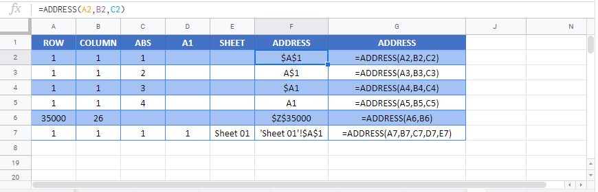
ADDRESS – Basic Example
Let’s say that we want to build a reference to the cell in 4th column and 1st row, aka cell D1. We can use the layout pictured here:
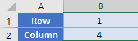
Our formula in A3 is simply
=ADDRESS(B1, B2)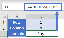
Note: By default the ADDRESS Function returns an absolute cell reference. By updating an optional argument we can change the cell references from absolute to relative. Let’s review this and other inputs to the ADDRESS Function…
ADDRESS Function Syntax and Inputs:
=ADDRESS(row_num,column_num,abs_num,C1,sheet_text)row_num – The row number for the reference. Example: 5 for row 5.
col_num – The column number for the reference. Example: 5 for Column E. You can not enter “E” for column E
abs_num – [optional] A number representing if the reference should have absolute or relative row/column references. 1 for absolute. 2 for absolute row/relative column. 3 for relative row/absolute column. 4 for relative.
a1 – [optional]. A number indicating whether to use standard (A1) cell reference format or R1C1 format. 1/TRUE for Standard (Default). 0/FALSE for R1C1.
sheet_text – [optional] The name of the worksheet to use. Defaults to current sheet.
ADDRESS with INDIRECT
We can combine ADDRESS with the INDIRECT Function. Consider this layout, where we have a list of items in column D.
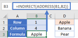
We can generate a reference to D1 like so
=ADDRESS(B1, B2)
=$D$1
By putting the address function inside an INDIRECT function, we’ll be able to use the generated cell reference and use it in a practical way. The INDIRECT will take the reference of “$D$1” and use it to fetch the value from that cell.
=INDIRECT(ADDRESS(B1, B2)
=INDIRECT($D$1)
="Apple"
Note: While the above gives a good example of making the ADDRESS Function useful, it’s not a good formula to use normally. It required two functions, and because of the INDIRECT it will be volatile in nature. A better alternative would have been to use the INDEX Function like this:
=INDEX(1:1048576, B1, B2)
Address of Specific Value
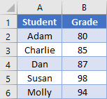
Sometimes when you have a large list of items, you need to know the location of an item in the list. Consider this table of scores from students. We’ve gone ahead and calculated the min, median, and max values of these scores in cells E2:G2.
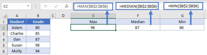
Let’s say we wanted to find these values. We have a two options:
- Filter our table for each of these items.
- Use the MATCH Function with ADDRESS. Remember that MATCH will return the relative position of a value within a range.
Our formula in E3 then is:
=ADDRESS(MATCH(E2, $B:$B, 0), 2)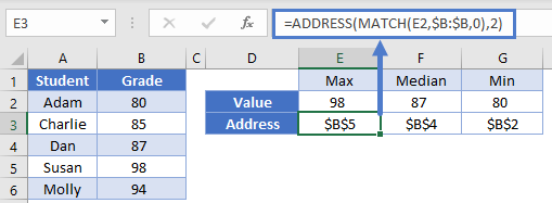
We can copy this same formula across to G3, and only the E2 reference will change since it’s the only relative reference. Looking back at E3, the MATCH function was able to find the value of 98 in the 5th row of column B. Our ADDRESS function then used this to build the full address of “$B$5”.
Translate Column Letters from Numbers
So far, all of the examples have returned an absolute reference. Let’s return a relative reference instead.
Below, in column B, we want to calculate the column letter corresponding to the column number in column A.
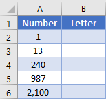
We will use the ADDRESS Function to return a reference on row 1 in relative format, and then we’ll remove the “1” from the text string so that we just have the letter(s) left. Consider in our table row 3, where our input is 13. Our formula in B3 is
=SUBSTITUTE(ADDRESS(1, A3, 4), "1", "")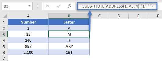
Note that we’ve given the 3rd argument within the ADDRESS function, which controls the relative vs. absolute referencing. The ADDRESS function will output “M1”, and then the SUBSTITUTE function removes the “1” so that we are left with just the “M”.
Find the Address of Named Ranges
In Excel, you can name range or ranges of cells, allowing you to simply refer to the named range instead of the cell reference.
Most named ranges are static, meaning they always refer to the same range. However, you can also create dynamic named ranges that change in size based on some formula(s).
With a dynamic named range, you might need to know the exact address that your named range is pointing to. We can do this with the ADDRESS Function.
In this example, we’ll look at how to define the address for our named range called “Grades”.
Let’s bring back our table from before:
To get the address of a range, you need to know the top left cell and the bottom left cell. The first part is easy enough to accomplish with the help of the ROW and COLUMN functions. Our formula in E1 can be
=ADDRESS(ROW(Grades), COLUMN(Grades))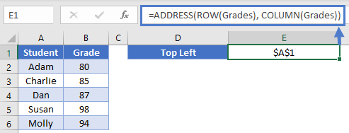
The ROW Function returns the row of the first cell in our range (which will be 1), and the COLUMN will do the same similarly for the column (also 1).
This formula will get the bottom-right cell
=ADDRESS(ROWS(Grades)-ROW(Grades)+1, COLUMNS(Grades)-COLUMN(Grades)+1)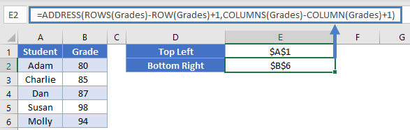
We used the ROWS and COLUMNS functions to calculate the height and width of the range. By subtracting the first row and column numbers, we calculate the last cell in the range
Finally, to put it all together into a single string, we can simply concatenate the values together with a colon in the middle. Formula in E3 can be
=E1 & ":" & E2
Note: While we were able to determine the address of the range, our ADDRESS function determined whether to list the references as relative or absolute. Your dynamic ranges will have relative references that this technique won’t pick up.
2nd Note: This technique only works on a continuous names range. If you had a named range that was defined as something like this formula
=A1:B2, A5:B6then the technique above would result in errors.
ADDRESS function in Google Sheets
The ADDRESS function works exactly the same in Google Sheets as in Excel.
ADDRESS function returns the address of a specific cell (text value) pointed to by the column and row numbers. For example, as a result of the function =ADDRESS(5;7), the value of $G$5 will be displayed.
Note: the presence of «$» characters in the $G$5 address indicates that the reference to this cell is absolute, that is, it does not change when copying data.
ADDRESS function in Excel: syntax features description
ADDRESS function has the following syntax entry:
=ADDRESS(Row_num, Column_num, [Abs_num], [A1], [Sheet_text])
The first two arguments of this function are required.
Argument Description:
- Row Number is a numeric value corresponding to the line number in which the required cell is located;
- Column number is a numeric value that corresponds to the column number in which the desired cell is located;
- [Abs_num] is a number from the range from 1 to 4, corresponding to one of the types of the returned cell reference:
- Absolute on all cell, for example — $A$4.
- Absolute only per line, for example — A$4.
- Absolute only per column, for example — $A4.
- Relative to the whole cell, for example A4.
- [A1] is a logical value that defines one of two types of links: A1 or R1C1;
- [Sheet_text] is a text value that defines the name of a sheet in an Excel document. Used to create external links.
Notes:
- References of type R1C1 are used to number columns and rows. To return links of this type, the logical value FALSE or the corresponding numeric value 0 must be explicitly specified as the a1 parameter.
- The link style in Excel can be changed by checking / unchecking the checkbox of the menu item “Link style R1C1”, which is located in “File — Options — Formulas — Working with Formulas”.
- If you need a reference to a cell that is located in another sheet of this Excel document, it is useful to use the [sheet_name] parameter, which takes a text value that corresponds to the name of the desired sheet, for example, «Sheet7».
Examples of using ADDRESS function in Excel
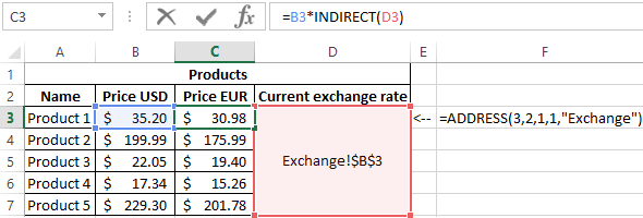
Example 1. The Excel spreadsheet contains a cell that displays dynamically changing data depending on certain conditions. To work with the actual data in the table, which is located on another sheet of the document, you need to get a link.
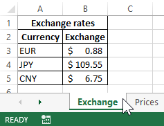
On the sheet «Exchange» created a table with the current exchange rates:
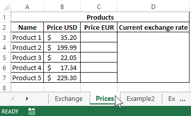
On a separate sheet “Prices”, a table with goods was created, displaying the value in US dollars (USD):
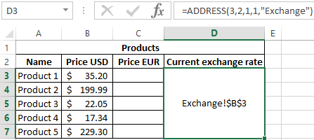
In D3 we place a link to a cell in the table located on the sheet “Exchange”, which contains information about the USD exchange rate. To do this, we introduce the following formula: =ADDRESS(3;2;1;1;»Exchange»).
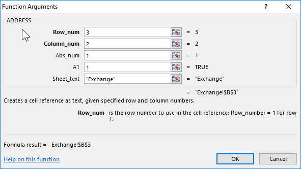
Parameter value:
- 3 — the number of the line containing the required cell;
- 2 — the column number with the desired cell;
- 1 — reference type is absolute;
- 1 — select the style of links with alphanumeric entry;
- “Exchange” is the name of the sheet on which the table with the desired cell is located.
To calculate the cost in Euro, we use the formula: =B3*INDIRECT(D3).
INDIRECT function is required to obtain a numeric value stored in the cell referenced. As a result of calculations for other products, we obtain the following table:
How to get the ADDRESS of the cell reference Excel?
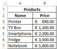
Example 2. The table contains data on the price of goods, sorted in ascending order of value. It is necessary to get links to cells with the minimum and maximum cost of goods, respectively.
The source table is as follows:
To get the reference to the cell with the minimum cost of the goods use the formula:
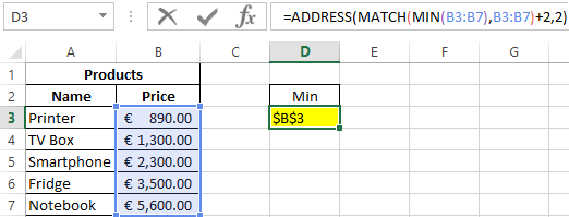
ADDRESS function accepts the following parameters:
- The number corresponding to the line number with the minimum price value (the MIN function searches for the minimum value and returns it; the MATCH function finds the position of the cell containing the minimum price value. Added 2 to the resulting value, because the MATCH searches for the range of selected cells.
- 2 — the number of the column in which the desired cell is located.
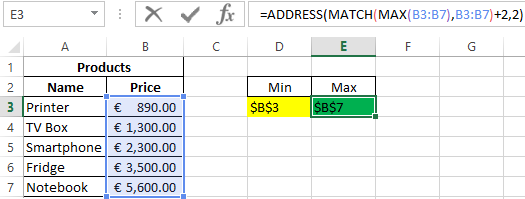
In a similar way we get a link to the cell with the maximum price of the goods. As a result, we get:
ADDRESS by row and column numbers of an Excel sheet in the style of R1C1
Example 3. The table contains a cell, the data from which is used in another software product. To ensure compatibility, you must provide a link to it in the form of R1C1.
The source table is as follows:
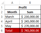
To get a reference to B6, we use the following formula: =ADDRESS(6;2;1;0).
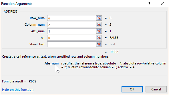
Function Arguments:
- 6 — line number of the desired cell;
- 2 — the number of the column containing;
- 1 — type of reference (absolute);
- 0 — an indication of the style R1C1.
As a result, we get the link:
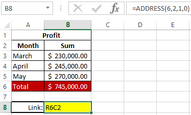
Practical application of the ADDRESS function: Searching of the value in a range Excel table in columns and rows.
Note: when using the R1C1 style, the absolute reference record does not contain the «$» sign. To distinguish between absolute and relative references, square brackets «[]» are used. For example, if in this example, as the type of link parameter, specify the number 4, the cell reference will look like this:
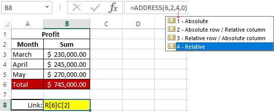
Download examples ADDRESS function for getting link to cell in Excel
This is the absolute type of links in rows and columns when using the R1C1 style.
На чтение 18 мин. Просмотров 74.6k.

сэр Артур Конан Дойл
Это большая ошибка — теоретизировать, прежде чем кто-то получит данные
Эта статья охватывает все, что вам нужно знать об использовании ячеек и диапазонов в VBA. Вы можете прочитать его от начала до конца, так как он сложен в логическом порядке. Или использовать оглавление ниже, чтобы перейти к разделу по вашему выбору.
Рассматриваемые темы включают свойство смещения, чтение
значений между ячейками, чтение значений в массивы и форматирование ячеек.
Содержание
- Краткое руководство по диапазонам и клеткам
- Введение
- Важное замечание
- Свойство Range
- Свойство Cells рабочего листа
- Использование Cells и Range вместе
- Свойство Offset диапазона
- Использование диапазона CurrentRegion
- Использование Rows и Columns в качестве Ranges
- Использование Range вместо Worksheet
- Чтение значений из одной ячейки в другую
- Использование метода Range.Resize
- Чтение Value в переменные
- Как копировать и вставлять ячейки
- Чтение диапазона ячеек в массив
- Пройти через все клетки в диапазоне
- Форматирование ячеек
- Основные моменты
Краткое руководство по диапазонам и клеткам
| Функция | Принимает | Возвращает | Пример | Вид |
| Range | адреса ячеек |
диапазон ячеек |
.Range(«A1:A4») | $A$1:$A$4 |
| Cells | строка, столбец |
одна ячейка |
.Cells(1,5) | $E$1 |
| Offset | строка, столбец |
диапазон | .Range(«A1:A2») .Offset(1,2) |
$C$2:$C$3 |
| Rows | строка (-и) | одна или несколько строк |
.Rows(4) .Rows(«2:4») |
$4:$4 $2:$4 |
| Columns | столбец (-цы) |
один или несколько столбцов |
.Columns(4) .Columns(«B:D») |
$D:$D $B:$D |
Введение
Это третья статья, посвященная трем основным элементам VBA. Этими тремя элементами являются Workbooks, Worksheets и Ranges/Cells. Cells, безусловно, самая важная часть Excel. Почти все, что вы делаете в Excel, начинается и заканчивается ячейками.
Вы делаете три основных вещи с помощью ячеек:
- Читаете из ячейки.
- Пишите в ячейку.
- Изменяете формат ячейки.
В Excel есть несколько методов для доступа к ячейкам, таких как Range, Cells и Offset. Можно запутаться, так как эти функции делают похожие операции.
В этой статье я расскажу о каждом из них, объясню, почему они вам нужны, и когда вам следует их использовать.
Давайте начнем с самого простого метода доступа к ячейкам — с помощью свойства Range рабочего листа.
Важное замечание
Я недавно обновил эту статью, сейчас использую Value2.
Вам может быть интересно, в чем разница между Value, Value2 и значением по умолчанию:
' Value2
Range("A1").Value2 = 56

' Value
Range("A1").Value = 56

' По умолчанию используется значение
Range("A1") = 56
Использование Value может усечь число, если ячейка отформатирована, как валюта. Если вы не используете какое-либо свойство, по умолчанию используется Value.
Лучше использовать Value2, поскольку он всегда будет возвращать фактическое значение ячейки.
Свойство Range
Рабочий лист имеет свойство Range, которое можно использовать для доступа к ячейкам в VBA. Свойство Range принимает тот же аргумент, что и большинство функций Excel Worksheet, например: «А1», «А3: С6» и т.д.
В следующем примере показано, как поместить значение в ячейку с помощью свойства Range.
Sub ZapisVYacheiku()

    ' Запишите число в ячейку A1 на листе 1 этой книги
    ThisWorkbook.Worksheets("Лист1").Range("A1").Value2 = 67

    ' Напишите текст в ячейку A2 на листе 1 этой рабочей книги
    ThisWorkbook.Worksheets("Лист1").Range("A2").Value2 = "Иван Петров"

    ' Запишите дату в ячейку A3 на листе 1 этой книги
    ThisWorkbook.Worksheets("Лист1").Range("A3").Value2 = #11/21/2019#

End Sub
Как видно из кода, Range является членом Worksheets, которая, в свою очередь, является членом Workbook. Иерархия такая же, как и в Excel, поэтому должно быть легко понять. Чтобы сделать что-то с Range, вы должны сначала указать рабочую книгу и рабочий лист, которому она принадлежит.
В оставшейся части этой статьи я буду использовать кодовое имя для ссылки на лист.

Следующий код показывает приведенный выше пример с использованием кодового имени рабочего листа, т.е. Лист1 вместо ThisWorkbook.Worksheets («Лист1»).
Sub IspKodImya ()

    ' Запишите число в ячейку A1 на листе 1 этой книги
     Sheet1.Range("A1").Value2 = 67

    ' Напишите текст в ячейку A2 на листе 1 этой рабочей книги
    Sheet1.Range("A2").Value2 = "Иван Петров"

    ' Запишите дату в ячейку A3 на листе 1 этой книги
    Sheet1.Range("A3").Value2 = #11/21/2019#

End Sub
Вы также можете писать в несколько ячеек, используя свойство
Range
Sub ZapisNeskol()

    ' Запишите число в диапазон ячеек
    Sheet1.Range("A1:A10").Value2 = 67

    ' Написать текст в несколько диапазонов ячеек
    Sheet1.Range("B2:B5,B7:B9").Value2 = "Иван Петров"

End Sub
Свойство Cells рабочего листа
У Объекта листа есть другое свойство, называемое Cells, которое очень похоже на Range . Есть два отличия:
- Cells возвращают диапазон только одной ячейки.
- Cells принимает строку и столбец в качестве аргументов.
В приведенном ниже примере показано, как записывать значения
в ячейки, используя свойства Range и Cells.
Sub IspCells()

    ' Написать в А1
    Sheet1.Range("A1").Value2 = 10
    Sheet1.Cells(1, 1).Value2  = 10

    ' Написать в А10
    Sheet1.Range("A10").Value2 = 10
    Sheet1.Cells(10, 1).Value2  = 10

    ' Написать в E1
    Sheet1.Range("E1").Value2 = 10
    Sheet1.Cells(1, 5).Value2  = 10

End Sub
Вам должно быть интересно, когда использовать Cells, а когда Range. Использование Range полезно для доступа к одним и тем же ячейкам при каждом запуске макроса.
Например, если вы использовали макрос для вычисления суммы и
каждый раз записывали ее в ячейку A10, тогда Range подойдет для этой задачи.
Использование свойства Cells полезно, если вы обращаетесь к
ячейке по номеру, который может отличаться. Проще объяснить это на примере.
В следующем коде мы просим пользователя указать номер столбца. Использование Cells дает нам возможность использовать переменное число для столбца.
Sub ZapisVPervuyuPustuyuYacheiku()

    Dim UserCol As Integer

    ' Получить номер столбца от пользователя
    UserCol = Application.InputBox("Пожалуйста, введите номер столбца...", Type:=1)

    ' Написать текст в выбранный пользователем столбец
    Sheet1.Cells(1, UserCol).Value2 = "Иван Петров"

End Sub
В приведенном выше примере мы используем номер для столбца,
а не букву.
Чтобы использовать Range здесь, потребуется преобразовать эти значения в ссылку на
буквенно-цифровую ячейку, например, «С1». Использование свойства Cells позволяет нам
предоставить строку и номер столбца для доступа к ячейке.
Иногда вам может понадобиться вернуть более одной ячейки, используя номера строк и столбцов. В следующем разделе показано, как это сделать.
Использование Cells и Range вместе
Как вы уже видели, вы можете получить доступ только к одной ячейке, используя свойство Cells. Если вы хотите вернуть диапазон ячеек, вы можете использовать Cells с Range следующим образом:
Sub IspCellsSRange()

    With Sheet1
        ' Запишите 5 в диапазон A1: A10, используя свойство Cells
        .Range(.Cells(1, 1), .Cells(10, 1)).Value2 = 5

        ' Диапазон B1: Z1 будет выделен жирным шрифтом
        .Range(.Cells(1, 2), .Cells(1, 26)).Font.Bold = True

    End With

End Sub
Как видите, вы предоставляете начальную и конечную ячейку
диапазона. Иногда бывает сложно увидеть, с каким диапазоном вы имеете дело,
когда значением являются все числа. Range имеет свойство Address, которое
отображает буквенно-цифровую ячейку для любого диапазона. Это может
пригодиться, когда вы впервые отлаживаете или пишете код.
В следующем примере мы распечатываем адрес используемых нами
диапазонов.
Sub PokazatAdresDiapazona()

    ' Примечание. Использование подчеркивания позволяет разделить строки кода.
    With Sheet1

        ' Запишите 5 в диапазон A1: A10, используя свойство Cells
        .Range(.Cells(1, 1), .Cells(10, 1)).Value2 = 5
        Debug.Print "Первый адрес: " _
            + .Range(.Cells(1, 1), .Cells(10, 1)).Address

        ' Диапазон B1: Z1 будет выделен жирным шрифтом
        .Range(.Cells(1, 2), .Cells(1, 26)).Font.Bold = True
        Debug.Print "Второй адрес : " _
            + .Range(.Cells(1, 2), .Cells(1, 26)).Address

    End With

End Sub
В примере я использовал Debug.Print для печати в Immediate Window. Для просмотра этого окна выберите «View» -> «в Immediate Window» (Ctrl + G).


Свойство Offset диапазона
У диапазона есть свойство, которое называется Offset. Термин «Offset» относится к отсчету от исходной позиции. Он часто используется в определенных областях программирования. С помощью свойства «Offset» вы можете получить диапазон ячеек того же размера и на определенном расстоянии от текущего диапазона. Это полезно, потому что иногда вы можете выбрать диапазон на основе определенного условия. Например, на скриншоте ниже есть столбец для каждого дня недели. Учитывая номер дня (т.е. понедельник = 1, вторник = 2 и т.д.). Нам нужно записать значение в правильный столбец.

Сначала мы попытаемся сделать это без использования Offset.
' Это Sub тесты с разными значениями
Sub TestSelect()

    ' Понедельник
    SetValueSelect 1, 111.21
    ' Среда
    SetValueSelect 3, 456.99
    ' Пятница
    SetValueSelect 5, 432.25
    ' Воскресение
    SetValueSelect 7, 710.17

End Sub

' Записывает значение в столбец на основе дня
Public Sub SetValueSelect(lDay As Long, lValue As Currency)

    Select Case lDay
        Case 1: Sheet1.Range("H3").Value2 = lValue
        Case 2: Sheet1.Range("I3").Value2 = lValue
        Case 3: Sheet1.Range("J3").Value2 = lValue
        Case 4: Sheet1.Range("K3").Value2 = lValue
        Case 5: Sheet1.Range("L3").Value2 = lValue
        Case 6: Sheet1.Range("M3").Value2 = lValue
        Case 7: Sheet1.Range("N3").Value2 = lValue
    End Select

End Sub
Как видно из примера, нам нужно добавить строку для каждого возможного варианта. Это не идеальная ситуация. Использование свойства Offset обеспечивает более чистое решение.
' Это Sub тесты с разными значениями
Sub TestOffset()

    DayOffSet 1, 111.01
    DayOffSet 3, 456.99
    DayOffSet 5, 432.25
    DayOffSet 7, 710.17

End Sub

Public Sub DayOffSet(lDay As Long, lValue As Currency)

    ' Мы используем значение дня с Offset, чтобы указать правильный столбец
    Sheet1.Range("G3").Offset(, lDay).Value2 = lValue

End Sub
Как видите, это решение намного лучше. Если количество дней увеличилось, нам больше не нужно добавлять код. Чтобы Offset был полезен, должна быть какая-то связь между позициями ячеек. Если столбцы Day в приведенном выше примере были случайными, мы не могли бы использовать Offset. Мы должны были бы использовать первое решение.
Следует иметь в виду, что Offset сохраняет размер диапазона. Итак .Range («A1:A3»).Offset (1,1) возвращает диапазон B2:B4. Ниже приведены еще несколько примеров использования Offset.
Sub IspOffset()

    ' Запись в В2 - без Offset
    Sheet1.Range("B2").Offset().Value2 = "Ячейка B2"

    ' Написать в C2 - 1 столбец справа
    Sheet1.Range("B2").Offset(, 1).Value2 = "Ячейка C2"

    ' Написать в B3 - 1 строка вниз
    Sheet1.Range("B2").Offset(1).Value2 = "Ячейка B3"

    ' Запись в C3 - 1 столбец справа и 1 строка вниз
    Sheet1.Range("B2").Offset(1, 1).Value2 = "Ячейка C3"

    ' Написать в A1 - 1 столбец слева и 1 строка вверх
    Sheet1.Range("B2").Offset(-1, -1).Value2 = "Ячейка A1"

    ' Запись в диапазон E3: G13 - 1 столбец справа и 1 строка вниз
    Sheet1.Range("D2:F12").Offset(1, 1).Value2 = "Ячейки E3:G13"

End Sub
Использование диапазона CurrentRegion
CurrentRegion возвращает диапазон всех соседних ячеек в данный диапазон. На скриншоте ниже вы можете увидеть два CurrentRegion. Я добавил границы, чтобы прояснить CurrentRegion.

Строка или столбец пустых ячеек означает конец CurrentRegion.
Вы можете вручную проверить
CurrentRegion в Excel, выбрав диапазон и нажав Ctrl + Shift + *.
Если мы возьмем любой диапазон
ячеек в пределах границы и применим CurrentRegion, мы вернем диапазон ячеек во
всей области.
Например:
Range («B3»). CurrentRegion вернет диапазон B3:D14
Range («D14»). CurrentRegion вернет диапазон B3:D14
Range («C8:C9»). CurrentRegion вернет диапазон B3:D14 и так далее
Как пользоваться
Мы получаем CurrentRegion следующим образом
' CurrentRegion вернет B3:D14 из приведенного выше примера
Dim rg As Range
Set rg = Sheet1.Range("B3").CurrentRegion
Только чтение строк данных
Прочитать диапазон из второй строки, т.е. пропустить строку заголовка.
' CurrentRegion вернет B3:D14 из приведенного выше примера
Dim rg As Range
Set rg = Sheet1.Range("B3").CurrentRegion

' Начало в строке 2 - строка после заголовка
Dim i As Long
For i = 2 To rg.Rows.Count
    ' текущая строка, столбец 1 диапазона
    Debug.Print rg.Cells(i, 1).Value2
Next i
Удалить заголовок
Удалить строку заголовка (т.е. первую строку) из диапазона. Например, если диапазон — A1:D4, это возвратит A2:D4
' CurrentRegion вернет B3:D14 из приведенного выше примера
Dim rg As Range
Set rg = Sheet1.Range("B3").CurrentRegion

' Удалить заголовок
Set rg = rg.Resize(rg.Rows.Count - 1).Offset(1)

' Начните со строки 1, так как нет строки заголовка
Dim i As Long
For i = 1 To rg.Rows.Count
    ' текущая строка, столбец 1 диапазона
    Debug.Print rg.Cells(i, 1).Value2
Next i
Использование Rows и Columns в качестве Ranges
Если вы хотите что-то сделать со всей строкой или столбцом,
вы можете использовать свойство «Rows и
Columns» на рабочем листе. Они оба принимают один параметр — номер строки
или столбца, к которому вы хотите получить доступ.
Sub IspRowIColumns()

    ' Установите размер шрифта столбца B на 9
    Sheet1.Columns(2).Font.Size = 9

    ' Установите ширину столбцов от D до F
    Sheet1.Columns("D:F").ColumnWidth = 4

    ' Установите размер шрифта строки 5 до 18
    Sheet1.Rows(5).Font.Size = 18

End Sub
Использование Range вместо Worksheet
Вы также можете использовать Cella, Rows и Columns, как часть Range, а не как часть Worksheet. У вас может быть особая необходимость в этом, но в противном случае я бы избегал практики. Это делает код более сложным. Простой код — твой друг. Это уменьшает вероятность ошибок.
Код ниже выделит второй столбец диапазона полужирным. Поскольку диапазон имеет только две строки, весь столбец считается B1:B2
Sub IspColumnsVRange()

    ' Это выделит B1 и B2 жирным шрифтом.
    Sheet1.Range("A1:C2").Columns(2).Font.Bold = True

End Sub
Чтение значений из одной ячейки в другую
В большинстве примеров мы записали значения в ячейку. Мы
делаем это, помещая диапазон слева от знака равенства и значение для размещения
в ячейке справа. Для записи данных из одной ячейки в другую мы делаем то же
самое. Диапазон назначения идет слева, а диапазон источника — справа.
В следующем примере показано, как это сделать:
Sub ChitatZnacheniya()

    ' Поместите значение из B1 в A1
    Sheet1.Range("A1").Value2 = Sheet1.Range("B1").Value2

    ' Поместите значение из B3 в лист2 в ячейку A1
    Sheet1.Range("A1").Value2 = Sheet2.Range("B3").Value2

    ' Поместите значение от B1 в ячейки A1 до A5
    Sheet1.Range("A1:A5").Value2 = Sheet1.Range("B1").Value2

    ' Вам необходимо использовать свойство «Value», чтобы прочитать несколько ячеек
    Sheet1.Range("A1:A5").Value2 = Sheet1.Range("B1:B5").Value2

End Sub
Как видно из этого примера, невозможно читать из нескольких ячеек. Если вы хотите сделать это, вы можете использовать функцию копирования Range с параметром Destination.
Sub KopirovatZnacheniya()

    ' Сохранить диапазон копирования в переменной
    Dim rgCopy As Range
    Set rgCopy = Sheet1.Range("B1:B5")

    ' Используйте это для копирования из более чем одной ячейки
    rgCopy.Copy Destination:=Sheet1.Range("A1:A5")

    ' Вы можете вставить в несколько мест назначения
    rgCopy.Copy Destination:=Sheet1.Range("A1:A5,C2:C6")

End Sub
Функция Copy копирует все, включая формат ячеек. Это тот же результат, что и ручное копирование и вставка выделения. Подробнее об этом вы можете узнать в разделе «Копирование и вставка ячеек»
Использование метода Range.Resize
При копировании из одного диапазона в другой с использованием присваивания (т.е. знака равенства) диапазон назначения должен быть того же размера, что и исходный диапазон.
Использование функции Resize позволяет изменить размер
диапазона до заданного количества строк и столбцов.
Например:
Sub ResizePrimeri()

    ' Печатает А1
    Debug.Print Sheet1.Range("A1").Address

    ' Печатает A1:A2
    Debug.Print Sheet1.Range("A1").Resize(2, 1).Address

    ' Печатает A1:A5
    Debug.Print Sheet1.Range("A1").Resize(5, 1).Address

    ' Печатает A1:D1
    Debug.Print Sheet1.Range("A1").Resize(1, 4).Address

    ' Печатает A1:C3
    Debug.Print Sheet1.Range("A1").Resize(3, 3).Address

End Sub
Когда мы хотим изменить наш целевой диапазон, мы можем
просто использовать исходный размер диапазона.
Другими словами, мы используем количество строк и столбцов
исходного диапазона в качестве параметров для изменения размера:
Sub Resize()

    Dim rgSrc As Range, rgDest As Range

    ' Получить все данные в текущей области
    Set rgSrc = Sheet1.Range("A1").CurrentRegion

      ' Получить диапазон назначения
    Set rgDest = Sheet2.Range("A1")
    Set rgDest = rgDest.Resize(rgSrc.Rows.Count, rgSrc.Columns.Count)

    rgDest.Value2 = rgSrc.Value2

End Sub
Мы можем сделать изменение размера в одну строку, если нужно:
Sub Resize2()

    Dim rgSrc As Range

    ' Получить все данные в ткущей области
    Set rgSrc = Sheet1.Range("A1").CurrentRegion

    With rgSrc
        Sheet2.Range("A1").Resize(.Rows.Count, .Columns.Count) = .Value2
    End With

End Sub
Чтение Value в переменные
Мы рассмотрели, как читать из одной клетки в другую. Вы также можете читать из ячейки в переменную. Переменная используется для хранения значений во время работы макроса. Обычно вы делаете это, когда хотите манипулировать данными перед тем, как их записать. Ниже приведен простой пример использования переменной. Как видите, значение элемента справа от равенства записывается в элементе слева от равенства.
Sub IspVar()

    ' Создайте
    Dim val As Integer

    ' Читать число из ячейки
    val = Sheet1.Range("A1").Value2

    ' Добавить 1 к значению
    val = val + 1

    ' Запишите новое значение в ячейку
    Sheet1.Range("A2").Value2 = val

End Sub
Для чтения текста в переменную вы используете переменную
типа String.
Sub IspVarText()

    ' Объявите переменную типа string
    Dim sText As String

    ' Считать значение из ячейки
    sText = Sheet1.Range("A1").Value2

    ' Записать значение в ячейку
    Sheet1.Range("A2").Value2 = sText

End Sub
Вы можете записать переменную в диапазон ячеек. Вы просто
указываете диапазон слева, и значение будет записано во все ячейки диапазона.
Sub VarNeskol()

    ' Считать значение из ячейки
    Sheet1.Range("A1:B10").Value2 = 66

End Sub
Вы не можете читать из нескольких ячеек в переменную. Однако
вы можете читать массив, который представляет собой набор переменных. Мы
рассмотрим это в следующем разделе.
Как копировать и вставлять ячейки
Если вы хотите скопировать и вставить диапазон ячеек, вам не
нужно выбирать их. Это распространенная ошибка, допущенная новыми пользователями
VBA.
Вы можете просто скопировать ряд ячеек, как здесь:
Range("A1:B4").Copy Destination:=Range("C5")
При использовании этого метода копируется все — значения,
форматы, формулы и так далее. Если вы хотите скопировать отдельные элементы, вы
можете использовать свойство PasteSpecial
диапазона.
Работает так:
Range("A1:B4").Copy
Range("F3").PasteSpecial Paste:=xlPasteValues
Range("F3").PasteSpecial Paste:=xlPasteFormats
Range("F3").PasteSpecial Paste:=xlPasteFormulas
В следующей таблице приведен полный список всех типов вставок.
| Виды вставок |
| xlPasteAll |
| xlPasteAllExceptBorders |
| xlPasteAllMergingConditionalFormats |
| xlPasteAllUsingSourceTheme |
| xlPasteColumnWidths |
| xlPasteComments |
| xlPasteFormats |
| xlPasteFormulas |
| xlPasteFormulasAndNumberFormats |
| xlPasteValidation |
| xlPasteValues |
| xlPasteValuesAndNumberFormats |
Чтение диапазона ячеек в массив
Вы также можете скопировать значения, присвоив значение
одного диапазона другому.
Range("A3:Z3").Value2 = Range("A1:Z1").Value2
Значение диапазона в этом примере считается вариантом массива. Это означает, что вы можете легко читать из диапазона ячеек в массив. Вы также можете писать из массива в диапазон ячеек. Если вы не знакомы с массивами, вы можете проверить их в этой статье.
В следующем коде показан пример использования массива с
диапазоном.
Sub ChitatMassiv()

    ' Создать динамический массив
    Dim StudentMarks() As Variant

    ' Считать 26 значений в массив из первой строки
    StudentMarks = Range("A1:Z1").Value2

    ' Сделайте что-нибудь с массивом здесь

    ' Запишите 26 значений в третью строку
    Range("A3:Z3").Value2 = StudentMarks

End Sub
Имейте в виду, что массив, созданный для чтения, является
двумерным массивом. Это связано с тем, что электронная таблица хранит значения
в двух измерениях, то есть в строках и столбцах.
Пройти через все клетки в диапазоне
Иногда вам нужно просмотреть каждую ячейку, чтобы проверить значение.
Вы можете сделать это, используя цикл For Each, показанный в следующем коде.
Sub PeremeschatsyaPoYacheikam()

    ' Пройдите через каждую ячейку в диапазоне
    Dim rg As Range
    For Each rg In Sheet1.Range("A1:A10,A20")
        ' Распечатать адрес ячеек, которые являются отрицательными
        If rg.Value < 0 Then
            Debug.Print rg.Address + " Отрицательно."
        End If
    Next

End Sub
Вы также можете проходить последовательные ячейки, используя
свойство Cells и стандартный цикл For.
Стандартный цикл более гибок в отношении используемого вами
порядка, но он медленнее, чем цикл For Each.
Sub PerehodPoYacheikam()

    ' Пройдите клетки от А1 до А10
    Dim i As Long
    For i = 1 To 10
        ' Распечатать адрес ячеек, которые являются отрицательными
        If Range("A" & i).Value < 0 Then
            Debug.Print Range("A" & i).Address + " Отрицательно."
        End If
    Next

    ' Пройдите в обратном порядке, то есть от A10 до A1
    For i = 10 To 1 Step -1
        ' Распечатать адрес ячеек, которые являются отрицательными
        If Range("A" & i) < 0 Then
            Debug.Print Range("A" & i).Address + " Отрицательно."
        End If
    Next

End Sub
Форматирование ячеек
Иногда вам нужно будет отформатировать ячейки в электронной
таблице. Это на самом деле очень просто. В следующем примере показаны различные
форматы, которые можно добавить в любой диапазон ячеек.
Sub FormatirovanieYacheek()

    With Sheet1

        ' Форматировать шрифт
        .Range("A1").Font.Bold = True
        .Range("A1").Font.Underline = True
        .Range("A1").Font.Color = rgbNavy

        ' Установите числовой формат до 2 десятичных знаков
        .Range("B2").NumberFormat = "0.00"
        ' Установите числовой формат даты
        .Range("C2").NumberFormat = "dd/mm/yyyy"
        ' Установите формат чисел на общий
        .Range("C3").NumberFormat = "Общий"
        ' Установить числовой формат текста
        .Range("C4").NumberFormat = "Текст"

        ' Установите цвет заливки ячейки
        .Range("B3").Interior.Color = rgbSandyBrown

        ' Форматировать границы
        .Range("B4").Borders.LineStyle = xlDash
        .Range("B4").Borders.Color = rgbBlueViolet

    End With

End Sub
Основные моменты
Ниже приводится краткое изложение основных моментов
- Range возвращает диапазон ячеек
- Cells возвращают только одну клетку
- Вы можете читать из одной ячейки в другую
- Вы можете читать из диапазона ячеек в другой диапазон ячеек.
- Вы можете читать значения из ячеек в переменные и наоборот.
- Вы можете читать значения из диапазонов в массивы и наоборот
- Вы можете использовать цикл For Each или For, чтобы проходить через каждую ячейку в диапазоне.
- Свойства Rows и Columns позволяют вам получить доступ к диапазону ячеек этих типов