
Excel for Microsoft 365 Excel 2021 Excel 2019 Excel 2016 Excel 2013 Excel 2010 Excel 2007 More…Less
Let’s say you need to create a grammatically correct sentence from several columns of data to prepare a mass mailing. Or, maybe you need to format numbers with text without affecting formulas that use those numbers. In Excel, there are several ways to combine text and numbers.
Use a number format to display text before or after a number in a cell
If a column that you want to sort contains both numbers and text—such as Product #15, Product #100, Product #200—it may not sort as you expect. You can format cells that contain 15, 100, and 200 so that they appear in the worksheet as Product #15, Product #100, and Product #200.
Use a custom number format to display the number with text—without changing the sorting behavior of the number. In this way, you change how the number appears without changing the value.
Follow these steps:
-
Select the cells that you want to format.
-
On the Home tab, in the Number group, click the arrow .

-
In the Category list, click a category such as Custom, and then click a built-in format that resembles the one that you want.
-
In the Type field, edit the number format codes to create the format that you want.
To display both text and numbers in a cell, enclose the text characters in double quotation marks (» «), or precede the numbers with a backslash ().
NOTE: Editing a built-in format does not remove the format.
|
To display |
Use this code |
How it works |
|---|---|---|
|
12 as Product #12 |
«Product # » 0 |
The text enclosed in the quotation marks (including a space) is displayed before the number in the cell. In the code, «0» represents the number contained in the cell (such as 12). |
|
12:00 as 12:00 AM EST |
h:mm AM/PM «EST» |
The current time is shown using the date/time format h:mm AM/PM, and the text «EST» is displayed after the time. |
|
-12 as $-12.00 Shortage and 12 as $12.00 Surplus |
$0.00 «Surplus»;$-0.00 «Shortage» |
The value is shown using a currency format. In addition, if the cell contains a positive value (or 0), «Surplus» is displayed after the value. If the cell contains a negative value, «Shortage» is displayed instead. |
Combine text and numbers from different cells into the same cell by using a formula
When you do combine numbers and text in a cell, the numbers become text and no longer function as numeric values. This means that you can no longer perform any math operations on them.
To combine numbers, use the CONCATENATE or CONCAT, TEXT or TEXTJOIN functions, and the ampersand (&) operator.
Notes:
-
In Excel 2016, Excel Mobile, and Excel for the web, CONCATENATE has been replaced with the CONCAT function. Although the CONCATENATE function is still available for backward compatibility, you should consider using CONCAT, because CONCATENATE may not be available in future versions of Excel.
-
TEXTJOIN combines the text from multiple ranges and/or strings, and includes a delimiter you specify between each text value that will be combined. If the delimiter is an empty text string, this function will effectively concatenate the ranges. TEXTJOIN is not available in Excel 2013 and previous versions.
Examples
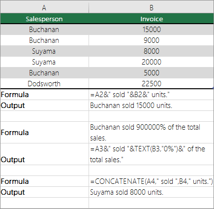
See various examples in the figure below.
Look closely at the use of the TEXT function in the second example in the figure. When you join a number to a string of text by using the concatenation operator, use the TEXT function to control the way the number is shown. The formula uses the underlying value from the referenced cell (.4 in this example) — not the formatted value you see in the cell (40%). You use the TEXT function to restore the number formatting.
Need more help?
You can always ask an expert in the Excel Tech Community or get support in the Answers community.
See Also
-
CONCATENATE function
-
CONCAT function
-
TEXT function
-
TEXTJOIN function
Need more help?
Want more options?
Explore subscription benefits, browse training courses, learn how to secure your device, and more.
Communities help you ask and answer questions, give feedback, and hear from experts with rich knowledge.
Содержание
- Convert numbers stored as text to numbers
- 1. Select a column
- 2. Click this button
- 3. Click Apply
- 4. Set the format
- Other ways to convert:
- 1. Insert a new column
- 2. Use the VALUE function
- 3. Rest your cursor here
- 4. Click and drag down
- Combine text and numbers
- Use a number format to display text before or after a number in a cell
- Combine text and numbers from different cells into the same cell by using a formula
- Examples
- Need more help?
- Number Formatting in Excel — All You Need to Know
- How to create a custom number format in Excel
- Basics
- Syntax
- Placeholders and the Cheat Sheet
- Common Practices
- Display and control of the first digit and decimals
- Add text to numbers
- Hide value
- Replace zeroes with dashes
- Start with zeroes
- Dealing with thousands, millions, and more
- Display numbers as phone numbers
- Showing Month and Weekday Names
- Come in Colors Everywhere
- Conditions
Convert numbers stored as text to numbers
Numbers that are stored as text can cause unexpected results, like an uncalculated formula showing instead of a result. Most of the time, Excel will recognize this and you’ll see an alert next to the cell where numbers are being stored as text. If you see the alert, select the cells, and then click  to choose a convert option.
Check out Format numbers to learn more about formatting numbers and text in Excel.

If the alert button is not available, do the following:
1. Select a column
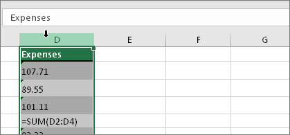
Select a column with this problem. If you don’t want to convert the whole column, you can select one or more cells instead. Just be sure the cells you select are in the same column, otherwise this process won’t work. (See «Other ways to convert» below if you have this problem in more than one column.)
2. Click this button
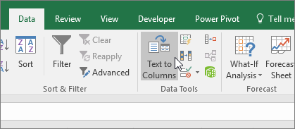
The Text to Columns button is typically used for splitting a column, but it can also be used to convert a single column of text to numbers. On the Data tab, click Text to Columns.
3. Click Apply
The rest of the Text to Columns wizard steps are best for splitting a column. Since you’re just converting text in a column, you can click Finish right away, and Excel will convert the cells.
4. Set the format

Press CTRL + 1 (or  + 1 on the Mac). Then select any format.
Note: If you still see formulas that are not showing as numeric results, then you may have Show Formulas turned on. Go to the Formulas tab and make sure Show Formulas is turned off.
Other ways to convert:
You can use the VALUE function to return just the numeric value of the text.
1. Insert a new column
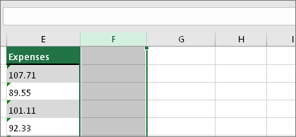
Insert a new column next to the cells with text. In this example, column E contains the text stored as numbers. Column F is the new column.
2. Use the VALUE function
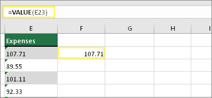
In one of the cells of the new column, type =VALUE() and inside the parentheses, type a cell reference that contains text stored as numbers. In this example it’s cell E23.
3. Rest your cursor here
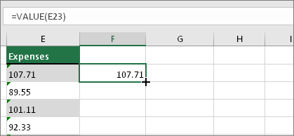
Now you’ll fill the cell’s formula down, into the other cells. If you’ve never done this before, here’s how to do it: Rest your cursor on the lower-right corner of the cell until it changes to a plus sign.
4. Click and drag down
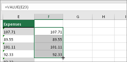
Click and drag down to fill the formula to the other cells. After that’s done, you can use this new column, or you can copy and paste these new values to the original column. Here’s how to do that: Select the cells with the new formula. Press CTRL + C. Click the first cell of the original column. Then on the Home tab, click the arrow below Paste, and then click Paste Special > Values.
If the steps above didn’t work, you can use this method, which can be used if you’re trying to convert more than one column of text.
Select a blank cell that doesn’t have this problem, type the number 1 into it, and then press Enter.
Press CTRL + C to copy the cell.
Select the cells that have numbers stored as text.
On the Home tab, click Paste > Paste Special.
Click Multiply, and then click OK. Excel multiplies each cell by 1, and in doing so, converts the text to numbers.
Press CTRL + 1 (or + 1 on the Mac). Then select any format.
Источник
Combine text and numbers
Let’s say you need to create a grammatically correct sentence from several columns of data to prepare a mass mailing. Or, maybe you need to format numbers with text without affecting formulas that use those numbers. In Excel, there are several ways to combine text and numbers.
Use a number format to display text before or after a number in a cell
If a column that you want to sort contains both numbers and text—such as Product #15, Product #100, Product #200—it may not sort as you expect. You can format cells that contain 15, 100, and 200 so that they appear in the worksheet as Product #15, Product #100, and Product #200.
Use a custom number format to display the number with text—without changing the sorting behavior of the number. In this way, you change how the number appears without changing the value.
Follow these steps:
Select the cells that you want to format.
On the Home tab, in the Number group, click the arrow .
In the Category list, click a category such as Custom, and then click a built-in format that resembles the one that you want.
In the Type field, edit the number format codes to create the format that you want.
To display both text and numbers in a cell, enclose the text characters in double quotation marks (» «), or precede the numbers with a backslash ().
NOTE: Editing a built-in format does not remove the format.
12 as Product #12
The text enclosed in the quotation marks (including a space) is displayed before the number in the cell. In the code, «0» represents the number contained in the cell (such as 12).
12:00 as 12:00 AM EST
The current time is shown using the date/time format h:mm AM/PM, and the text «EST» is displayed after the time.
-12 as $-12.00 Shortage and 12 as $12.00 Surplus
$0.00 «Surplus»;$-0.00 «Shortage»
The value is shown using a currency format. In addition, if the cell contains a positive value (or 0), «Surplus» is displayed after the value. If the cell contains a negative value, «Shortage» is displayed instead.
Combine text and numbers from different cells into the same cell by using a formula
When you do combine numbers and text in a cell, the numbers become text and no longer function as numeric values. This means that you can no longer perform any math operations on them.
To combine numbers, use the CONCATENATE or CONCAT, TEXT or TEXTJOIN functions, and the ampersand (&) operator.
In Excel 2016, Excel Mobile, and Excel for the web, CONCATENATE has been replaced with the CONCAT function. Although the CONCATENATE function is still available for backward compatibility, you should consider using CONCAT, because CONCATENATE may not be available in future versions of Excel.
TEXTJOIN combines the text from multiple ranges and/or strings, and includes a delimiter you specify between each text value that will be combined. If the delimiter is an empty text string, this function will effectively concatenate the ranges. TEXTJOIN is not available in Excel 2013 and previous versions.
Examples
See various examples in the figure below.
Look closely at the use of the TEXT function in the second example in the figure. When you join a number to a string of text by using the concatenation operator, use the TEXT function to control the way the number is shown. The formula uses the underlying value from the referenced cell (.4 in this example) — not the formatted value you see in the cell (40%). You use the TEXT function to restore the number formatting.
Need more help?
You can always ask an expert in the Excel Tech Community or get support in the Answers community.
Источник
Number Formatting in Excel — All You Need to Know
by Adam | Apr 2, 2018 | Blog

If you used Excel in any shape or form, there is a pretty good chance that you’ve used the formatting and number formatting features. Formatting options like number, currency, percentage, date and time values are easily accessible to users. However, that’s not all there is in the world of text and number formatting. Going down the rabbit hole, custom formatting can help you fully configure Excel’s built-in settings for formatting.
The main advantage of this approach is that you can alter the look of your data without changing the actual values. This means that you do not need to use additional spaces or formulas to create the layout you want and preserve the raw data.
If you want to modify your data anyways, or need to change a value inside a formula, you can use the TEXT function with all custom formatting syntax we are going to cover in this article. It should be noted that the TEXT function returns a text, and the return value cannot be used in mathematical calculations. If you do, you will receive a #VALUE! error. In this article we’re going to be using a workbook template. You can download it below.
How to create a custom number format in Excel
- Select the cell to be formatted and press Ctrl+1 to open the Format Cells dialog. An alternative way to do is by right-clicking the cell and then going to Format Cells > Number Tab.
- Under Category, select Custom.
- Type in the format code into the Type
- Click OK to save your changes.
Note: In Format Cells dialog you can modify the built-in format codes by selecting the format you want to modify in its own category (i.e. Currency > ($1,234.10)) and then selecting Custom Category. Don’t worry, Excel will not let you delete built-in formats.

Basics
Syntax
The format code has 4 sections separated by semicolons.
POSITIVE; NEGATIVE; ZERO; TEXT
These sections are optional,
- If a code contains only 1 section, the format is applied to all number types — positive, negative and zero.
- If a code contains 2 sections, the first section is used for positive and zero values, while the second section is applied to negative values.
- If a code contains 3 sections, the first is for positive, the second is for negative, and the third is for zero.
- A code only affects text values if all sections exist.
Default format type in Excel is called General. You can type General for sections you don’t want formatted. Make sure you use a minus sign (-) with General if you want to skip negative values.
If you want to completely hide a type, leave it blank after the semicolon. For example; to hide 0 values, General;-General;;General
Placeholders and the Cheat Sheet
| Placeholder | Description | Raw Value | Format Code | Formatted Value |
| General | Default format | 1234.567 | General | 1234.567 |
| # | Placeholder for digits (numbers) and does not add any leading zeroes. | 1234.567 | #####.#### | 1234.567 |
| 0 | Placeholder for digits (numbers) and add any leading zeroes. | 1234.567 | 00000.0000 | 01234.5670 |
| ? | Placeholder for digits (numbers) and add space characters. | 1234.567 | . | 1234.567 |
| . | Placeholder for the decimal place. | 1234.567 | 0.00 | 1234.57 |
| _ | Adds a blank space, to the width of the following character. You can use in combination with parentheses to add left and right indents, _( and _) respectively. | 99 | _(#_);(#) | 99 |
| -25 | (25) | |||
| 58 | 58 | |||
| 12 | 12 | |||
| -71 | (71) | |||
| 36 | 36 | |||
| * | Repeats the character after asterisk until the width of the cell is filled. | 66 | 0 *! | 66 . |
| Full Name | @ *_ | Full Name ____ | ||
| % | Convert value to a percentage with % sign | 0.12 | % | 12% |
| , | Thousands separator | 1234.567 | #, | 1 |
| 12345678 | #, | 12,346 | ||
| 12345678 | #,###, | 12,346 | ||
| 12345678 | #,, | 12 | ||
| E | Scientific notation format. Requires a ‘+’ symbol after, and a digit placeholder before and after. | 1234.567 | 0.00E+00 | 1.23E+03 |
| / | Represents fractions | 1.234 | # ##/## | 1 11/47 |
| 1.234 | # 000/000 | 1 117/500 | ||
| 1.234 | ##/## | 58/47 | ||
| «» | Text placeholder for multiple characters | 1234.567 | #,##0 «km/h» | 1,235 km/h |
| Good | «Result is: «@ | Result is: Good | ||
| Text placeholder for single character | 1234 | #.00, K | 1.23 K | |
| 1234567 | #.00,, M | 1.23 M | ||
| @ | Placeholder for text | Bad | «Result is: «@ | Result is: Bad |
| [color] | Change Color of value. Options: [Black], [Green], [White], [Blue], [Magenta], [Yellow], [Cyan], [Red] | 1234.567 | [Green]#,##0.00_); [Red](#,##0.00); [Blue]0.00_); [Magenta]@ |
1,234.57 |
| -1234.567 | (1,234.57) | |||
| 0 | 0.00 | |||
| This is a text | This is a text |
Common Practices
Display and control of the first digit and decimals
Decimal places in the code are indicated with a period (.). Number of zeroes after the period (.) define the number of decimal places. For example,
- 0 — display 1 decimal place
- 00 — display 2 decimal places
If the number has more decimals than the decimal placeholders defined, the number will be rounded to the nearest number of placeholders.
| Raw Value | Format Code | Formatted Value |
| 123.4 | 0.0 | 123.4 |
| 123.4 | 0.00 | 123.40 |
| 123.45 | 0.00 | 123.45 |
| 123.45 | 0.00 | 123.46 |
| 123.456 | 0.0 | 123.5 |
Alternatively, hash (#) and question mark (?) symbols can be used as decimal places. However, because any missing decimal places will be filled with zeroes, using zeroes instead will be easier to read.
| Raw Value | Format Code | Formatted Value |
| 0.25 | 0.00 | 0.25 |
| 0.25 | #.## | .25 |
| 123 | 0.00 | 123.0 |
| 123 | #. | 123.00 |
| 123 | #.## | 123. |
Add text to numbers
Custom text can be added to the beginning or the end of a value. Text and characters should be added inside quotes («») and backslashes (). You can use backslash () to add single character.
| Raw Value | Format Code | Formatted Value |
| 123.4 | 0.0 «ft.» | 123.4 ft. |
| 123.4 | 0.00 l | 123.40 l |
| 123.45 | «Approx.» 0 | Approx. 123 |
| 123.45 | «Result:» 0.00 C | Result: 123.46 C |
| Bad | «Result is: «@ | Result is: Bad |
Quotation marks or backslashes are not necessary for spaces ( ) and some special characters.
| Symbol | Description |
| + and — | Plus and minus signs |
| ( ) | Left and right parenthesis |
| : | Colon |
| ^ | Caret |
| ‘ | Apostrophe |
| Curly brackets | |
| Less-than and greater than signs | |
| = | Equal sign |
| / | Forward slash |
| ! | Exclamation point |
| & | Ampersand |
| Tilde | |
| Space character |
Below are some special characters you can use by copying or typing in the numerical code while pressing down Alt button.
| Symbol | Code | Description |
| ™ | Alt+0153 | Trademark |
| © | Alt+0169 | Copyright symbol |
| ° | Alt+0176 | Degree symbol |
| ± | Alt+0177 | Plus-Minus sign |
| µ | Alt+0181 | Micro sign |
Hide value
If you leave any number of sections blank, the value of those sections will be hidden. A section should always be separated (defined) by a semicolon (;). Here are some examples,
| Raw Value | Format Code | Formatted Value |
| 1 | 0;;0; | 1 |
| -2 | 0;;0; | |
| 0 | 0;;0; | 0 |
| Some text | 0;;0; | |
| 1 | ;(0);;@ | |
| -2 | ;(0);;@ | (2) |
| 0 | ;(0);;@ | |
| Some text | ;(0);;@ | Some Text |
| 1 | ;;; | |
| -2 | ;;; | |
| 0 | ;;; | |
| Some text | ;;; |
Replace zeroes with dashes
Zeroes can make data tables look more complicated than they actually are. You can hide them completely by using the previous method, or replace them with any character of your choice. Dash (-) is a common example. All you need to is place a dash into the ‘Zero section’.
| Raw Value | Format Code | Formatted Value |
| 0 | General;-General;»-«;General | — |
| 3487 | General;-General;»-«;»-« | — |
| 12 | #,##0.00;(#,##0.00);»-«; | — |
Start with zeroes
If try to enter a ZIP number that starts with 0, the leading zeroes will be removed automatically by Excel. To keep the leading zeros, use zero (0) placeholder for whole numbers.
| Raw Value | Format Code | Formatted Value |
| 10010 | 00000 | 10010 |
| 3487 | 00000 | 03487 |
| 12 | 00000 | 00012 |
| 0 | 00000 | 00000 |
| 123456 | 00000 | 123456 |
Dealing with thousands, millions, and more
You may have noticed that ‘0.0’ or other simple formats do not separate thousands or millions. Adding a comma into the code will insert commas to separate numbers.
| Raw Value | Format Code | Formatted Value |
| 1234 | #,##0 | 1,234 |
| 123456 | #,##0 | 123,456 |
| 12345678 | #,##0 | 12,345,678 |
| 123456.789 | #,##0 | 123,457 |
| 123456.789 | #,##0.0 | 123,456.8 |
There must be placeholders for numbers smaller than one thousand, otherwise such values will be hidden. This behavior allows us to round and format our value to show only thousands or millions.
| Raw Value | Format Code | Formatted Value |
| 1234 | #, | 1 |
| 123456 | #, | 123 |
| 12345678 | #, | 12345 |
| 12345678 | #,, | 12 |
| 123456 | #.0, K | 123.5 K |
| 12345678 | #.0,, M | 12.3 M |
Display numbers as phone numbers
Phone numbers can be hard to read without any separators. Custom Number Format Codes is perfect for this job. The hash (#) character should be your best bet to avoid any redundancy of placeholders (0, ?)
| Raw Value | Format Code | Formatted Value |
| 1234567890 | (###) ###-#### | (123) 456-7890 |
| 12345678900 | (###) #### #### | (123) 4567 8900 |
| 1234567890 | (##) #### #### | (12) 3456 7890 |
Showing Month and Weekday Names
Date and time values are stored as numbers in Excel. When you enter a date, Excel automatically converts it into a numerical value, and then formats the cell.
Before jumping into the code, let’s review some basics. Formatting code has special placeholders for date and time formatting that behave a bit differently. For example, while m and mm will show month as a number, mmm and mmmm will show as a text string. Below are some examples.
| Raw Value | Format Code | Formatted Value |
| 4/1/2018 | m | 4 |
| 4/1/2018 | mm | 04 |
| 4/1/2018 | mmm | Apr |
| 4/1/2018 | mmmm | April |
| 4/1/2018 | mmmmm | A |
| 4/1/2018 | d | 1 |
| 4/1/2018 | dd | 01 |
| 4/1/2018 | ddd | Sun |
| 4/1/2018 | dddd | Sunday |
| 4/1/2018 11:59:31 PM | dddd, mmmm dd, yyyy h:mm AM/PM;@ | Sunday, April 01, 2018 11:59 PM |
Here is the full list of options for the date 4/1/2018 23:59:31 ,
| Format Code | Description | Example (4/1/2018 23:59:31) |
| yyyy | Displays the year as a four-digit number. | 2018 |
| yy | Displays the year as a two-digit number. | 18 |
| m | Displays the month as a number without a leading zero. | 4 |
| mm | Displays the month with a leading zero. | 04 |
| mmm | Displays the month as text, as an abbreviation. | Apr |
| mmmm | Displays the month as text. | April |
| mmmmm | Displays the month as a single character | A |
| d | Displays the day as a number, without a leading zero. | 1 |
| dd | Displays the day as a number, with a leading zero. | 01 |
| ddd | Displays the day as a day of the week, as an abbreviation. | Sun |
| dddd | Displays the day as a day of the week, without abbreviation | Sunday |
| h | Displays the hour without a leading zero. | 23 |
| hh | Displays the hour with a leading zero. | 23 |
| [h] | Displays elapsed time in hours (to be used when the time value exceeds 24 hours). | 1036607 |
| m | Displays the minute without a leading zero. | 4 |
| mm | Displays the minute with a leading zero. | 04 |
| [m] | Displays elapsed time in minutes (to be used when the time value exceeds 60 minutes). | 62196479 |
| s | Displays the second without a leading zero. | 31 |
| ss | with a leading zero. | 31 |
| [s] | Displays elapsed time in seconds (to be used when the time value exceeds 60 seconds). | 3731788771 |
| AM/PM | Converts to 12-hour time. Displays either AM/am/A/a or PM/pm/P/p depending on the time of day. | PM |
| am/pm | pm | |
| A/P | P | |
| a/p | p |
Come in Colors Everywhere
Number Formatting can be used color sections of a code. A common example is using the color red for negative numbers. Color code must be placed inside square brackets (i.e. [color]), and entered at the beginning of a section. Here are some available colors,
- [Black]
- [Blue]
- [Cyan]
- [Green]
- [Magenta]
- [Red]
- [White]
- [Yellow]
| Raw Value | Format Code | Formatted Value |
| 1234.567 | [Green]#,##0.00_);[Red](#,##0.00);[Blue]0.00);[Magenta]@ | 1,234.57 |
| -1234.567 | (1,234.57) | |
| 0 | 0.00 | |
| This is a text | This is a text |
Conditions
Although Excel has conditional formatting menu, basic conditions can be applied through code. Condition should be placed inside square brackets (i.e. [condition]) just like colors. Conditions are similar to the conditions in some functions (i.e. SUMIF). First add a logical operator, and then a value. For example, “[>=1000000]” means “if value of cell is greater than or equal to 1,000,000 apply the following format”. Conditions should come before the actual code, again, just like with colors. If you want to a color as well, the color code should come first.
Another important thing to note here is, that section structure changes from Positive, Negative, Zero, Text to First Condition, Second Condition (if exists), if previous conditions are not applied. There should be at least two sections for conditions.
If you enter only one condition code and then save the format, Excel will automatically add the second section with «;General». This means that if the condition is not met, General format will be used.
Источник
Helper Columns
The fastest way to approach problems like this is often to use helper columns to break the problem down. To do math on the numerical portions, I extracted the numbers.

You can get the locations of everything from the position of the R. In column B, I extracted the L number. B1:
=MID(A1,2,FIND("R",A1)-3)*1
MID extracts the characters starting with the second, for a length of the R position minus 3 (i.e., minus the L, -, and R). That is extracted as a string, so multiplying by 1 turns it into a number.
The R number is in column C. C1:
=MID(A1,FIND("R",A1)+1,LEN(A1))*1
In this case, MID starts at the position after the R, and takes the rest of the string. The number of characters is specified as the entire length of the A1 value, but Excel runs out of characters when it comes to the end of the string.
An alternate way to get the R number is the approach used in Rajesh S’s answer:
=REPLACE(A1,1,FIND("R",A1),"")*1
This replaces all of the characters to the left of the number, from the first through the R, with nothing. Again, the *1 converts the result to a numerical value.
The result in A8 is generated by building the new string using & to concatenate the pieces, plugging in the helper column sums:
="L" & SUM(B1:B6) & "-R" & SUM(C1:C6)
You can hide the helper columns or stick them out of the way if you don’t want them visible.
Without helper columns
Once you’ve figured out how to do it with helper columns, you can often eliminate the helper columns by using the formula in an array-style calculation. SUMPRODUCT lets you do that with a regular formula; it calculates the result for each value in the range, then sums them up. The sum of the L values can be done directly with:
=SUMPRODUCT(--(MID(A1:A6,2,FIND("R",A1:A6)-3)))
This is the same formula used for the helper column, but the single cell reference is replaced with the data range. This also illustrates another method for converting the text result to a number; Instead of *1, it uses a double negative to treat the result as a number while leaving its sign unchanged.
Similarly, for the R number, I’ll use the alternate formula because it’s a little shorter:
=SUMPRODUCT(--(REPLACE(A1:A6,1,FIND("R",A1:A6),"")))
Those formulas give you the sums without needing the helper columns. You can build the final result in a single cell by using these sums instead of the SUM(B1:B6) and SUM(C1:C6) that used the helper column results:
="L" & SUMPRODUCT(--(MID(A1:A6,2,FIND("R",A1:A6)-3))) & "-R" & SUMPRODUCT(--(REPLACE(A1:A6,1,FIND("R",A1:A6),"")))
Dynamic answer on another sheet
To have an automatically updated result replicated on another sheet, just put, in that display cell, a reference to the original result. You include the sheet name in the cell reference, connected by an exclamation mark. To refer to the result in cell A8 of Sheet1, the cell reference would be =Sheet1!A8.
A fast way to create the cell reference is to type = in the display cell, then before hitting Enter, go to the first sheet and click on the result cell. Excel will fill in the cell reference for you.
My NodeJS program populates an excel formula in a cell which in turn calculates the sum of all the numbers in a column. The numbers are stored as text in the cells.
The formula used is : =SUM(0+(I5:I19999)).
All the numbers are present in column ‘I’ but not necessarily till 19999th row (few may be blank).
However, the result of this formula is always #VALUE!.
I can’t seem to find the issue in this.
Any help in this issue is really appreciated.
Thanks!
asked Sep 25, 2017 at 8:03
![]()
7
Formula you are using to add numbers stored as text i.e. =SUM(0+(I5:I19999)) is an array formula and needs to be committed by pressing Ctrl+Shift+Enter.
If you want non-array formula you can use
=SUMPRODUCT((I5:I19999)*1)
answered Sep 25, 2017 at 8:58
![]()
MrigMrig
11.6k2 gold badges13 silver badges27 bronze badges
1
the value in the cell must be stored as a number because sum works on numbers only if you give text then it will display #VALUE.
you can store value as numbers using numformat(‘0.00’).you can get more info from this page https://support.office.com/en-us/article/Number-format-codes-5026bbd6-04bc-48cd-bf33-80f18b4eae68.if you are reading then you have to convert it.
Could you please let me know which package(exceljs,Node-xlsx) are you using so that i can send you the code require?
answered Sep 25, 2017 at 9:13
![]()
Introduction
Number formats control how numbers are displayed in Excel. The key benefit of number formats is that they change how a number looks without changing any data. They are a great way to save time in Excel because they perform a huge amount of formatting automatically. As a bonus, they make worksheets look more consistent and professional.
Video: What is a number format
What can you do with custom number formats?
Custom number formats can control the display of numbers, dates, times, fractions, percentages, and other numeric values. Using custom formats, you can do things like format dates to show month names only, format large numbers in millions or thousands, and display negative numbers in red.

Where can you use custom number formats?
Many areas in Excel support number formats. You can use them in tables, charts, pivot tables, formulas, and directly on the worksheet.
- Worksheet — format cells dialog
- Pivot Tables — via value field settings
- Charts — data labels and axis options
- Formulas — via the TEXT function
What is a number format?
A number format is a special code to control how a value is displayed in Excel. For example, the table below shows 7 different number formats applied to the same date, January 1, 2019:
| Input | Code | Result |
|---|---|---|
| 1-Jan-2019 | yyyy | 2019 |
| 1-Jan-2019 | yy | 19 |
| 1-Jan-2019 | mmm | Jan |
| 1-Jan-2019 | mmmm | January |
| 1-Jan-2019 | d | 1 |
| 1-Jan-2019 | ddd | Tue |
| 1-Jan-2019 | dddd | Tuesday |
The key thing to understand is that number formats change the way numeric values are displayed, but they do not change the actual values.
Where can you find number formats?
On the home tab of the ribbon, you’ll find a menu of build-in number formats. Below this menu to the right, there is a small button to access all number formats, including custom formats:

This button opens the Format Cells dialog box. You’ll find a complete list of number formats, organized by category, on the Number tab:

Note: you can open Format Cells dialog box with the keyboard shortcut Control + 1.
General is default
By default, cells start with the General format applied. The display of numbers using the General number format is somewhat «fluid». Excel will display as many decimal places as space allows, and will round decimals and use scientific number format when space is limited. The screen below shows the same values in column B and D, but D is narrower and Excel makes adjustments on the fly.

How to change number formats
You can select standard number formats (General, Number, Currency, Accounting, Short Date, Long Date, Time, Percentage, Fraction, Scientific, Text) on the home tab of the ribbon using the Number Format menu.
Note: As you enter data, Excel will sometimes change number formats automatically. For example if you enter a valid date, Excel will change to «Date» format. If you enter a percentage like 5%, Excel will change to Percentage, and so on.
Shortcuts for number formats
Excel provides a number of keyboard shortcuts for some common formats:
| Format | Shortcut |
|---|---|
| General format | Ctrl Shift ~ |
| Currency format | Ctrl Shift $ |
| Percentage format | Ctrl Shift % |
| Scientific format | Ctrl Shift ^ |
| Date format | Ctrl Shift # |
| Time format | Ctrl Shift @ |
| Custom formats | Control + 1 |
See also: 222 Excel Shortcuts for Windows and Mac
Where to enter custom formats
At the bottom of the predefined formats, you’ll see a category called custom. The Custom category shows a list of codes you can use for custom number formats, along with an input area to enter codes manually in various combinations.

When you select a code from the list, you’ll see it appear in the Type input box. Here you can modify existing custom code, or to enter your own codes from scratch. Excel will show a small preview of the code applied to the first selected value above the input area.
Note: Custom number formats live in a workbook, not in Excel generally. If you copy a value formatted with a custom format from one workbook to another, the custom number format will be transferred into the workbook along with the value.
How to create a custom number format
To create custom number format follow this simple 4-step process:
- Select cell(s) with values you want to format
- Control + 1 > Numbers > Custom
- Enter codes and watch preview area to see result
- Press OK to save and apply
Tip: if you want base your custom format on an existing format, first apply the base format, then click the «Custom» category and edit codes as you like.
How to edit a custom number format
You can’t really edit a custom number format per se. When you change an existing custom number format, a new format is created and will appear in the list in the Custom category. You can use the Delete button to delete custom formats you no longer need.
Warning: there is no «undo» after deleting a custom number format!
Structure and Reference
Excel custom number formats have a specific structure. Each number format can have up to four sections, separated with semi-colons as follows:

This structure can make custom number formats look overwhelmingly complex. To read a custom number format, learn to spot the semi-colons and mentally parse the code into these sections:
- Positive values
- Negative values
- Zero values
- Text values
Not all sections required
Although a number format can include up to four sections, only one section is required. By default, the first section applies to positive numbers, the second section applies to negative numbers, the third section applies to zero values, and the fourth section applies to text.
- When only one format is provided, Excel will use that format for all values.
- If you provide a number format with just two sections, the first section is used for positive numbers and zeros, and the second section is used for negative numbers.
- To skip a section, include a semi-colon in the proper location, but don’t specify a format code.
Characters that display natively
Some characters appear normally in a number format, while others require special handling. The following characters can be used without any special handling:
| Character | Comment |
|---|---|
| $ | Dollar |
| +- | Plus, minus |
| () | Parentheses |
| {} | Curly braces |
| <> | Less than, greater than |
| = | Equal |
| : | Colon |
| ^ | Caret |
| ‘ | Apostrophe |
| / | Forward slash |
| ! | Exclamation point |
| & | Ampersand |
| ~ | Tilde |
| Space character |
Escaping characters
Some characters won’t work correctly in a custom number format without being escaped. For example, the asterisk (*), hash (#), and percent (%) characters can’t be used directly in a custom number format – they won’t appear in the result. The escape character in custom number formats is the backslash (). By placing the backslash before the character, you can use them in custom number formats:
| Value | Code | Result |
|---|---|---|
| 100 | #0 | #100 |
| 100 | *0 | *100 |
| 100 | %0 | %100 |
Placeholders
Certain characters have special meaning in custom number format codes. The following characters are key building blocks:
| Character | Purpose |
|---|---|
| 0 | Display insignificant zeros |
| # | Display significant digits |
| ? | Display aligned decimals |
| . | Decimal point |
| , | Thousands separator |
| * | Repeat following character |
| _ | Add space |
| @ | Placeholder for text |
Zero (0) is used to force the display of insignificant zeros when a number has fewer digits than zeros in the format. For example, the custom format 0.00 will display zero as 0.00, 1.1 as 1.10 and .5 as 0.50.

Pound sign (#) is a placeholder for optional digits. When a number has fewer digits than # symbols in the format, nothing will be displayed. For example, the custom format #.## will display 1.15 as 1.15 and 1.1 as 1.1.

Question mark (?) is used to align digits. When a question mark occupies a place not needed in a number, a space will be added to maintain visual alignment.

Period (.) is a placeholder for the decimal point in a number. When a period is used in a custom number format, it will always be displayed, regardless of whether the number contains decimal values.
Comma (,) is a placeholder for the thousands separators in the number being displayed. It can be used to define the behavior of digits in relation to the thousands or millions digits.

Asterisk (*) is used to repeat characters. The character immediately following an asterisk will be repeated to fill remaining space in a cell.

Underscore (_) is used to add space in a number format. The character immediately following an underscore character controls how much space to add. A common use of the underscore character is to add space to align positive and negative values when a number format is adding parentheses to negative numbers only. For example, the number format «0_);(0)» is adding a bit of space to the right of positive numbers so that they stay aligned with negative numbers, which are enclosed in parentheses.

At (@) — placeholder for text. For example, the following number format will display text values in blue:
0;0;0;[Blue]@
See below for more information about using color.
Automatic rounding
It’s important to understand that Excel will perform «visual rounding» with all custom number formats. When a number has more digits than placeholders on the right side of the decimal point, the number is rounded to the number of placeholders. When a number has more digits than placeholders on the left side of the decimal point, extra digits are displayed. This is a visual effect only; actual values are not modified.
Number formats for TEXT
To display both text along with numbers, enclose the text in double quotes («»). You can use this approach to append or prepend text strings in a custom number format, as shown in the table below.
| Value | Code | Result |
|---|---|---|
| 10 | General» units» | 10 units |
| 10 | 0.0″ units» | 10.0 units |
| 5.5 | 0.0″ feet» | 5.5 feet |
| 30000 | 0″ feet» | 30000 feet |
| 95.2 | «Score: «0.0 | Score: 95.2 |
| 1-Jun | «Date: «mmmm d | Date: June 1 |
Number formats for DATES
Dates in Excel are just numbers, so you can use custom number formats to change the way they display. Excel has many specific codes you can use to display components of a date in different ways. The screen below shows how Excel displays the date in D5, September 3, 2018, with a variety of custom number formats:

Number formats for TIME
Times in Excel are fractional parts of a day. For example, 12:00 PM is 0.5, and 6:00 PM is 0.75. You can use the following codes in custom time formats to display components of a time in different ways. The screen below shows how Excel displays the time in D5, 9:35:07 AM, with a variety of custom number formats:

Note: m and mm can’t be used alone in a custom number format since they conflict with the month number code in date format codes.
Number formats for ELAPSED TIME
Elapsed time is a special case and needs special handling. By using square brackets, Excel provides a special way to display elapsed hours, minutes, and seconds. The following screen shows how Excel displays elapsed time based on the value in D5, which represents 1.25 days:

Number formats for COLORS
Excel provides basic support for colors in custom number formats. The following 8 colors can be specified by name in a number format: [black] [white] [red][green] [blue] [yellow] [magenta] [cyan]. Color names must appear in brackets.

Colors by index
In addition to color names, it’s also possible to specify colors by an index number (Color1,Color2,Color3, etc.) The examples below are using the custom number format: [ColorX]0″▲▼», where X is a number between 1-56:
[Color1]0"▲▼" // black
[Color2]0"▲▼" // white
[Color3]0"▲▼" // red
[Color4]0"▲▼" // green
etc.
The triangle symbols have been added only to make the colors easier to see. The first image shows all 56 colors on a standard white background. The second image shows the same colors on a gray background. Note the first 8 colors shown correspond to the named color list above.


Apply number formats in a formula
Although most number formats are applied directly to cells in a worksheet, you can also apply number formats inside a formula with the TEXT function. For example, with a valid date in A1, the following formula will display the month name only:
=TEXT(A1,"mmmm")
The result of the TEXT function is always text, so you are free to concatenate the result of TEXT to other strings:
="The contract expires in "&TEXT(A1,"mmmm")
The screen below shows the number formats in column C being applied to numbers in column B using the TEXT function:

One quirk of the TEXT function relates to double quotes («») that are part of certain custom number formats. Because the format_text is entered as a text string, Excel won’t allow you to enter the formula without removing the quotes or adding more quotes. For example, to display a large number in thousands, you can use a custom number format like this:
0, "k"Notice k appears in quotes («k»). To apply the same format with the TEXT function, you can use simply:
=TEXT(A1,"0, k")Notice the k is not surrounded by quotes. Alternately, you can add extra double quotes as below, which returns the same result:
=TEXT(A1,"0,""K""")This behavior only occurs when you are hardcoding a format inside TEXT. If you are applying a format entered elsewhere on the worksheet (as in cells C6 and C9 in the worksheet above) you can use a standard number format.
Measurements
You can use a custom number format to display numbers with an inches mark («) or a feet mark (‘). In the screen below, the number formats used for inches and feet are:
0.00 ' // feet
0.00 " // inches

These results are simplistic, and can’t be combined in a single number format. You can however use a formula to display feet together with inches.
Conditionals
Custom number formats also up to two conditions, which are written in square brackets like [>100] or [<=100]. When you use conditionals in custom number formats, you override the standard [positive];[negative];[zero];[text] structure. For example, to display values below 100 in red, you can use:
[Red][<100]0;0
To display values greater than or equal to 100 in blue, you can extend the format like this:
[Red][<100]0;[Blue][>=100]0

To apply more than two conditions, or to change other cell attributes, like fill color, etc. you’ll need to switch to Conditional Formatting, which can apply formatting with much more power and flexibility using formulas.
Plural text labels
You can use conditionals to add an «s» to labels greater than zero with a custom format like this:
[=1]0″ day»;0″ days»

Telephone numbers
Custom number formats can also be used for telephone numbers, as shown in the screen below:

Notice the third and fourth examples use a conditional format to check for numbers that contain an area code. If you have data that contains phone numbers with hard-coded punctuation (parentheses, hyphens, etc.) you will need to clean the telephone numbers first so that they only contain numbers.
Hide all content
You can actually use a custom number format to hide all content in a cell. The code is simply three semi-colons and nothing else ;;;
To reveal the content again, you can use the keyboard shortcut Control + Shift + ~, which applies the General format.
Other resources
- Developer Bryan Braun built a nice interactive tool for building custom number formats