Excel add if yes - Word и Excel - помощь в работе с программами

IF function

The IF function is one of the most popular functions in Excel, and it allows you to make logical comparisons between a value and what you expect.

So an IF statement can have two results. The first result is if your comparison is True, the second if your comparison is False.

For example, =IF(C2=”Yes”,1,2) says IF(C2 = Yes, then return a 1, otherwise return a 2).

Use the IF function, one of the logical functions, to return one value if a condition is true and another value if it’s false.

IF(logical_test, value_if_true, [value_if_false])

For example:

=IF(A2>B2,»Over Budget»,»OK»)
=IF(A2=B2,B4-A4,»»)

Argument name	Description
logical_test (required)	The condition you want to test.
value_if_true (required)	The value that you want returned if the result of *logical_test* is TRUE.
value_if_false (optional)	The value that you want returned if the result of *logical_test* is FALSE.

Simple IF examples

=IF(C2=”Yes”,1,2)

In the above example, cell D2 says: IF(C2 = Yes, then return a 1, otherwise return a 2)

=IF(C2=1,”Yes”,”No”)

In this example, the formula in cell D2 says: IF(C2 = 1, then return Yes, otherwise return No)As you see, the IF function can be used to evaluate both text and values. It can also be used to evaluate errors. You are not limited to only checking if one thing is equal to another and returning a single result, you can also use mathematical operators and perform additional calculations depending on your criteria. You can also nest multiple IF functions together in order to perform multiple comparisons.

=IF(C2>B2,”Over Budget”,”Within Budget”)

In the above example, the IF function in D2 is saying IF(C2 Is Greater Than B2, then return “Over Budget”, otherwise return “Within Budget”)

=IF(C2>B2,C2-B2,0)

In the above illustration, instead of returning a text result, we are going to return a mathematical calculation. So the formula in E2 is saying IF(Actual is Greater than Budgeted, then Subtract the Budgeted amount from the Actual amount, otherwise return nothing).

=IF(E7=”Yes”,F5*0.0825,0)

In this example, the formula in F7 is saying IF(E7 = “Yes”, then calculate the Total Amount in F5 * 8.25%, otherwise no Sales Tax is due so return 0)

Note: If you are going to use text in formulas, you need to wrap the text in quotes (e.g. “Text”). The only exception to that is using TRUE or FALSE, which Excel automatically understands.

Common problems

Problem	What went wrong
0 (zero) in cell	There was no argument for either value_if_true or value_if_False arguments. To see the right value returned, add argument text to the two arguments, or add TRUE or FALSE to the argument.
#NAME? in cell	This usually means that the formula is misspelled.

Need more help?

You can always ask an expert in the Excel Tech Community or get support in the Answers community.

Что возвращает функция

Заданное вами значение при выполнении двух условий ИСТИНА или ЛОЖЬ.

Синтаксис

=IF(logical_test, [value_if_true], [value_if_false]) — английская версия

=ЕСЛИ(лог_выражение; [значение_если_истина]; [значение_если_ложь]) — русская версия

Аргументы функции

logical_test (лог_выражение) — это условие, которое вы хотите протестировать. Этот аргумент функции должен быть логичным и определяемым как ЛОЖЬ или ИСТИНА. Аргументом может быть как статичное значение, так и результат функции, вычисления;
[value_if_true] ([значение_если_истина]) — (не обязательно) — это то значение, которое возвращает функция. Оно будет отображено в случае, если значение которое вы тестируете соответствует условию ИСТИНА;
[value_if_false] ([значение_если_ложь]) — (не обязательно) — это то значение, которое возвращает функция. Оно будет отображено в случае, если условие, которое вы тестируете соответствует условию ЛОЖЬ.

Дополнительная информация

В функции ЕСЛИ может быть протестировано 64 условий за один раз;
Если какой-либо из аргументов функции является массивом — оценивается каждый элемент массива;
Если вы не укажете условие аргумента FALSE (ЛОЖЬ) value_if_false (значение_если_ложь) в функции, т.е. после аргумента value_if_true (значение_если_истина) есть только запятая (точка с запятой), функция вернет значение “0”, если результат вычисления функции будет равен FALSE (ЛОЖЬ).
На примере ниже, формула =IF(A1> 20,”Разрешить”) или =ЕСЛИ(A1>20;»Разрешить») , где value_if_false (значение_если_ложь) не указано, однако аргумент value_if_true (значение_если_истина) по-прежнему следует через запятую. Функция вернет “0” всякий раз, когда проверяемое условие не будет соответствовать условиям TRUE (ИСТИНА).

|
Если вы не укажете условие аргумента TRUE(ИСТИНА) (value_if_true (значение_если_истина)) в функции, т.е. условие указано только для аргумента value_if_false (значение_если_ложь), то формула вернет значение “0”, если результат вычисления функции будет равен TRUE (ИСТИНА);
На примере ниже формула равна =IF (A1>20;«Отказать») или =ЕСЛИ(A1>20;»Отказать»), где аргумент value_if_true (значение_если_истина) не указан, формула будет возвращать “0” всякий раз, когда условие соответствует TRUE (ИСТИНА).

Функция Если в Excel примеры с несколькими условиями

Пример 1. Проверяем простое числовое условие с помощью функции IF (ЕСЛИ)

При использовании функции ЕСЛИ в Excel, вы можете использовать различные операторы для проверки состояния. Вот список операторов, которые вы можете использовать:

Ниже приведен простой пример использования функции при расчете оценок студентов. Если сумма баллов больше или равна «35», то формула возвращает “Сдал”, иначе возвращается “Не сдал”.

Пример 2. Использование вложенной функции IF (ЕСЛИ) для проверки условия выражения

Функция может принимать до 64 условий одновременно. Несмотря на то, что создавать длинные вложенные функции нецелесообразно, то в редких случаях вы можете создать формулу, которая множество условий последовательно.

В приведенном ниже примере мы проверяем два условия.

Первое условие проверяет, сумму баллов не меньше ли она чем 35 баллов. Если это ИСТИНА, то функция вернет “Не сдал”;
В случае, если первое условие — ЛОЖЬ, и сумма баллов больше 35, то функция проверяет второе условие. В случае если сумма баллов больше или равна 75. Если это правда, то функция возвращает значение “Отлично”, в других случаях функция возвращает “Сдал”.

Пример 3. Вычисляем сумму комиссии с продаж с помощью функции IF (ЕСЛИ) в Excel

Функция позволяет выполнять вычисления с числами. Хороший пример использования — расчет комиссии продаж для торгового представителя.

В приведенном ниже примере, торговый представитель по продажам:

не получает комиссионных, если объем продаж меньше 50 тыс;
получает комиссию в размере 2%, если продажи между 50-100 тыс
получает 4% комиссионных, если объем продаж превышает 100 тыс.

Рассчитать размер комиссионных для торгового агента можно по следующей формуле:

=IF(B2<50,0,IF(B2<100,B2*2%,B2*4%)) — английская версия

=ЕСЛИ(B2<50;0;ЕСЛИ(B2<100;B2*2%;B2*4%)) — русская версия

В формуле, использованной в примере выше, вычисление суммы комиссионных выполняется в самой функции ЕСЛИ. Если объем продаж находится между 50-100K, то формула возвращает B2 * 2%, что составляет 2% комиссии в зависимости от объема продажи.

Больше лайфхаков в нашем Telegram Подписаться

Пример 4. Используем логические операторы (AND/OR) (И/ИЛИ) в функции IF (ЕСЛИ) в Excel

Вы можете использовать логические операторы (AND/OR) (И/ИЛИ) внутри функции для одновременного тестирования нескольких условий.

Например, предположим, что вы должны выбрать студентов для стипендий, основываясь на оценках и посещаемости. В приведенном ниже примере учащийся имеет право на участие только в том случае, если он набрал более 80 баллов и имеет посещаемость более 80%.

Вы можете использовать функцию AND (И) вместе с функцией IF (ЕСЛИ), чтобы сначала проверить, выполняются ли оба эти условия или нет. Если условия соблюдены, функция возвращает “Имеет право”, в противном случае она возвращает “Не имеет право”.

Формула для этого расчета:

=IF(AND(B2>80,C2>80%),”Да”,”Нет”) — английская версия

=ЕСЛИ(И(B2>80;C2>80%);»Да»;»Нет») — русская версия

Пример 5. Преобразуем ошибки в значения “0” с помощью функции IF (ЕСЛИ)

С помощью этой функции вы также можете убирать ячейки содержащие ошибки. Вы можете преобразовать значения ошибок в пробелы или нули или любое другое значение.

Формула для преобразования ошибок в ячейках следующая:

=IF(ISERROR(A1),0,A1) — английская версия

=ЕСЛИ(ЕОШИБКА(A1);0;A1) — русская версия

Формула возвращает “0”, в случае если в ячейке есть ошибка, иначе она возвращает значение ячейки.

ПРИМЕЧАНИЕ. Если вы используете Excel 2007 или версии после него, вы также можете использовать функцию IFERROR для этого.

Точно так же вы можете обрабатывать пустые ячейки. В случае пустых ячеек используйте функцию ISBLANK, на примере ниже:

=IF(ISBLANK(A1),0,A1) — английская версия

=ЕСЛИ(ЕПУСТО(A1);0;A1) — русская версия

Источник

This Excel tutorial explains how to use the Excel IF function with syntax and examples.

Description

The Microsoft Excel IF function returns one value if the condition is TRUE, or another value if the condition is FALSE.

The IF function is a built-in function in Excel that is categorized as a Logical Function. It can be used as a worksheet function (WS) in Excel. As a worksheet function, the IF function can be entered as part of a formula in a cell of a worksheet.

If you want to follow along with this tutorial, download the example spreadsheet.

Download Example

Syntax

The syntax for the IF function in Microsoft Excel is:

IF( condition, value_if_true, [value_if_false] )

Parameters or Arguments

condition: The value that you want to test.
value_if_true: It is the value that is returned if condition evaluates to TRUE.
value_if_false: Optional. It is the value that is returned if condition evaluates to FALSE.

Returns

The IF function returns value_if_true when the condition is TRUE.
The IF function returns value_if_false when the condition is FALSE.
The IF function returns FALSE if the value_if_false parameter is omitted and the condition is FALSE.

Example (as Worksheet Function)

Let’s explore how to use the IF function as a worksheet function in Microsoft Excel.

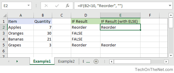
Based on the Excel spreadsheet above, the following IF examples would return:

=IF(B2<10, "Reorder", "")
Result: "Reorder"

=IF(A2="Apples", "Equal", "Not Equal")
Result: "Equal"

=IF(B3>=20, 12, 0)
Result: 12

Combining the IF function with Other Logical Functions

Quite often, you will need to specify more complex conditions when writing your formula in Excel. You can combine the IF function with other logical functions such as AND, OR, etc. Let’s explore this further.

AND function

The IF function can be combined with the AND function to allow you to test for multiple conditions. When using the AND function, all conditions within the AND function must be TRUE for the condition to be met. This comes in very handy in Excel formulas.

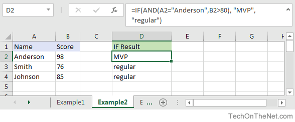
Based on the spreadsheet above, you can combine the IF function with the AND function as follows:

=IF(AND(A2="Anderson",B2>80), "MVP", "regular")
Result: "MVP"

=IF(AND(B2>=80,B2<=100), "Great Score", "Not Bad")
Result: "Great Score"

=IF(AND(B3>=80,B3<=100), "Great Score", "Not Bad")
Result: "Not Bad"

=IF(AND(A2="Anderson",A3="Smith",A4="Johnson"), 100, 50)
Result: 100

=IF(AND(A2="Anderson",A3="Smith",A4="Parker"), 100, 50)
Result: 50

In the examples above, all conditions within the AND function must be TRUE for the condition to be met.

OR function

The IF function can be combined with the OR function to allow you to test for multiple conditions. But in this case, only one or more of the conditions within the OR function needs to be TRUE for the condition to be met.

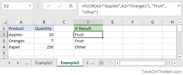
Based on the spreadsheet above, you can combine the IF function with the OR function as follows:

=IF(OR(A2="Apples",A2="Oranges"), "Fruit", "Other")
Result: "Fruit"

=IF(OR(A4="Apples",A4="Oranges"),"Fruit","Other")
Result: "Other"

=IF(OR(A4="Bananas",B4>=100), 999, "N/A")
Result: 999

=IF(OR(A2="Apples",A3="Apples",A4="Apples"), "Fruit", "Other")
Result: "Fruit"

In the examples above, only one of the conditions within the OR function must be TRUE for the condition to be met.

Let’s take a look at one more example that involves ranges of percentages.

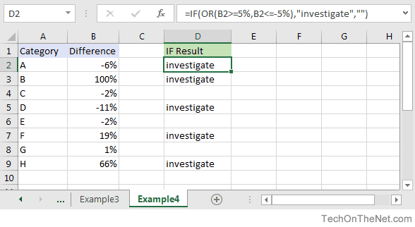
Based on the spreadsheet above, we would have the following formula in cell D2:

=IF(OR(B2>=5%,B2<=-5%),"investigate","")
Result: "investigate"

This IF function would return «investigate» if the value in cell B2 was either below -5% or above 5%. Since -6% is below -5%, it will return «investigate» as the result. We have copied this formula into cells D3 through D9 to show you the results that would be returned.

For example, in cell D3, we would have the following formula:

=IF(OR(B3>=5%,B3<=-5%),"investigate","")
Result: "investigate"

This formula would also return «investigate» but this time, it is because the value in cell B3 is greater than 5%.

Frequently Asked Questions

Question: In Microsoft Excel, I’d like to use the IF function to create the following logic:

if C11>=620, and C10=»F»or»S», and C4<=$1,000,000, and C4<=$500,000, and C7<=85%, and C8<=90%, and C12<=50, and C14<=2, and C15=»OO», and C16=»N», and C19<=48, and C21=»Y», then reference cell A148 on Sheet2. Otherwise, return an empty string.

Answer: The following formula would accomplish what you are trying to do:

=IF(AND(C11>=620, OR(C10="F",C10="S"), C4<=1000000, C4<=500000, C7<=0.85, C8<=0.9, C12<=50, C14<=2, C15="OO", C16="N", C19<=48, C21="Y"), Sheet2!A148, "")

Question: In Microsoft Excel, I’m trying to use the IF function to return 0 if cell A1 is either < 150,000 or > 250,000. Otherwise, it should return A1.

Answer: You can use the OR function to perform an OR condition in the IF function as follows:

=IF(OR(A1<150000,A1>250000),0,A1)

In this example, the formula will return 0 if cell A1 was either less than 150,000 or greater than 250,000. Otherwise, it will return the value in cell A1.

Question: In Microsoft Excel, I’m trying to use the IF function to return 25 if cell A1 > 100 and cell B1 < 200. Otherwise, it should return 0.

Answer: You can use the AND function to perform an AND condition in the IF function as follows:

=IF(AND(A1>100,B1<200),25,0)

In this example, the formula will return 25 if cell A1 is greater than 100 and cell B1 is less than 200. Otherwise, it will return 0.

Question: In Microsoft Excel, I need to write a formula that works this way:

IF (cell A1) is less than 20, then times it by 1,
IF it is greater than or equal to 20 but less than 50, then times it by 2
IF its is greater than or equal to 50 and less than 100, then times it by 3
And if it is great or equal to than 100, then times it by 4

Answer: You can write a nested IF statement to handle this. For example:

=IF(A1<20, A1*1, IF(A1<50, A1*2, IF(A1<100, A1*3, A1*4)))

Question: In Microsoft Excel, I need a formula in cell C5 that does the following:

IF A1+B1 <= 4, return $20
IF A1+B1 > 4 but <= 9, return $35
IF A1+B1 > 9 but <= 14, return $50
IF A1+B1 >= 15, return $75

Answer: In cell C5, you can write a nested IF statement that uses the AND function as follows:

=IF((A1+B1)<=4,20,IF(AND((A1+B1)>4,(A1+B1)<=9),35,IF(AND((A1+B1)>9,(A1+B1)<=14),50,75)))

Question: In Microsoft Excel, I need a formula that does the following:

IF the value in cell A1 is BLANK, then return «BLANK»
IF the value in cell A1 is TEXT, then return «TEXT»
IF the value in cell A1 is NUMERIC, then return «NUM»

Answer: You can write a nested IF statement that uses the ISBLANK function, the ISTEXT function, and the ISNUMBER function as follows:

=IF(ISBLANK(A1)=TRUE,"BLANK",IF(ISTEXT(A1)=TRUE,"TEXT",IF(ISNUMBER(A1)=TRUE,"NUM","")))

Question: In Microsoft Excel, I want to write a formula for the following logic:

IF R1<0.3 AND R2<0.3 AND R3<0.42 THEN «OK» OTHERWISE «NOT OK»

Answer: You can write an IF statement that uses the AND function as follows:

=IF(AND(R1<0.3,R2<0.3,R3<0.42),"OK","NOT OK")

Question: In Microsoft Excel, I need a formula for the following:

IF cell A1= PRADIP then value will be 100
IF cell A1= PRAVIN then value will be 200
IF cell A1= PARTHA then value will be 300
IF cell A1= PAVAN then value will be 400

Answer: You can write an IF statement as follows:

=IF(A1="PRADIP",100,IF(A1="PRAVIN",200,IF(A1="PARTHA",300,IF(A1="PAVAN",400,""))))

Question: In Microsoft Excel, I want to calculate following using an «if» formula:

if A1<100,000 then A1*.1% but minimum 25
and if A1>1,000,000 then A1*.01% but maximum 5000

Answer: You can write a nested IF statement that uses the MAX function and the MIN function as follows:

=IF(A1<100000,MAX(25,A1*0.1%),IF(A1>1000000,MIN(5000,A1*0.01%),""))

Question: In Microsoft Excel, I am trying to create an IF statement that will repopulate the data from a particular cell if the data from the formula in the current cell equals 0. Below is my attempt at creating an IF statement that would populate the data; however, I was unsuccessful.

=IF(IF(ISERROR(M24+((L24-S24)/AA24)),"0",M24+((L24-S24)/AA24)))=0,L24)

The initial part of the formula calculates the EAC (Estimate At completion = AC+(BAC-EV)/CPI); however if the current EV (Earned Value) is zero, the EAC will equal zero. IF the outcome is zero, I would like the BAC (Budget At Completion), currently recorded in another cell (L24), to be repopulated in the current cell as the EAC.

Answer: You can write an IF statement that uses the OR function and the ISERROR function as follows:

=IF(OR(S24=0,ISERROR(M24+((L24-S24)/AA24))),L24,M24+((L24-S24)/AA24))

Question: I have been looking at your Excel IF, AND and OR sections and found this very helpful, however I cannot find the right way to write a formula to express if C2 is either 1,2,3,4,5,6,7,8,9 and F2 is F and F3 is either D,F,B,L,R,C then give a value of 1 if not then 0. I have tried many formulas but just can’t get it right, can you help please?

Answer: You can write an IF statement that uses the AND function and the OR function as follows:

=IF(AND(C2>=1,C2<=9, F2="F",OR(F3="D",F3="F",F3="B",F3="L",F3="R",F3="C")),1,0)

Question:In Excel, I have a roadspeed of a car in m/s in cell A1 and a drop down menu of different units in C1 (which unclude mph and kmh). I have used the following IF function in B1 to convert the number to the unit selected from the dropdown box:

=IF(C1="mph","=A1*2.23693629",IF(C1="kmh","A1*3.6"))

However say if kmh was selected B1 literally just shows A1*3.6 and does not actually calculate it. Is there away to get it to calculate it instead of just showing the text message?

Answer: You are very close with your formula. Because you are performing mathematical operations (such as A1*2.23693629 and A1*3.6), you do not need to surround the mathematical formulas in quotes. Quotes are necessary when you are evaluating strings, not performing math.

Try the following:

=IF(C1="mph",A1*2.23693629,IF(C1="kmh",A1*3.6))

Question:For an IF statement in Excel, I want to combine text and a value.

For example, I want to put an equation for work hours and pay. IF I am paid more than I should be, I want it to read how many hours I owe my boss. But if I work more than I am paid for, I want it to read what my boss owes me (hours*Pay per Hour).

I tried the following:

=IF(A2<0,"I owe boss" abs(A2) "Hours","Boss owes me" abs(A2)*15 "dollars")

Is it possible or do I have to do it in 2 separate cells? (one for text and one for the value)

Answer: There are two ways that you can concatenate text and values. The first is by using the & character to concatenate:

=IF(A2<0,"I owe boss " & ABS(A2) & " Hours","Boss owes me " & ABS(A2)*15 &  " dollars")

Or the second method is to use the CONCATENATE function:

=IF(A2<0,CONCATENATE("I owe boss ", ABS(A2)," Hours"), CONCATENATE("Boss owes me ", ABS(A2)*15,  " dollars"))

Question:I have Excel 2000. IF cell A2 is greater than or equal to 0 then add to C1. IF cell B2 is greater than or equal to 0 then subtract from C1. IF both A2 and B2 are blank then equals C1. Can you help me with the IF function on this one?

Answer: You can write a nested IF statement that uses the AND function and the ISBLANK function as follows:

=IF(AND(ISBLANK(A2)=FALSE,A2>=0),C1+A2, IF(AND(ISBLANK(B2)=FALSE,B2>=0),C1-B2, IF(AND(ISBLANK(A2)=TRUE, ISBLANK(B2)=TRUE),C1,"")))

Question:How would I write this equation in Excel? IF D12<=0 then D12*L12, IF D12 is > 0 but <=600 then D12*F12, IF D12 is >600 then ((600*F12)+((D12-600)*E12))

Answer: You can write a nested IF statement as follows:

=IF(D12<=0,D12*L12,IF(D12>600,((600*F12)+((D12-600)*E12)),D12*F12))

Question:In Excel, I have this formula currently:

=IF(OR(A1>=40, B1>=40, C1>=40), "20", (A1+B1+C1)-20)

If one of my salesman does sale for $40-$49, then his commission is $20; however if his/her sale is less (for example $35) then the commission is that amount minus $20 ($35-$20=$15). I have 3 columns that are needed based on the type of sale. Only one column per row will be needed. The problem is that, when left blank, the total in the formula cell is -20. I need help setting up this formula so that when the 3 columns are left blank, the cell with the formula is left blank as well.

Answer: Using the AND function and the ISBLANK function, you can write your IF statement as follows:

=IF(AND(ISBLANK(A1),ISBLANK(B1),ISBLANK(C1)),"",IF(OR(A1>40, B1>40, C1>40), "20", (A1+B1+C1)-20))

In this formula, we are using the ISBLANK function to check if all 3 cells A1, B1, and C1 are blank, and if they are return a blank value («»). Then the rest is the formula that you originally wrote.

Question:In Excel, I need to create a simple booking and and out system, that shows a date out and a date back

«A1» = allows person to input date booked out
«A2» =allows person to input date booked back in

«A3″= shows status of product, eg, booked out, overdue return etc.

I can automate A3 with the following IF function:

=IF(ISBLANK(A2),"booked out","returned")

But what I cant get to work is if the product is out for 10 days or more, I would like the cell to say «send email»

Can you assist?

Answer: Using the TODAY function and adding an additional IF function, you can write your formula as follows:

=IF(ISBLANK(A2),IF(TODAY()-A1>10,"send email","booked out"),"returned")

Question:Using Microsoft Excel, I need a formula in cell U2 that does the following:

IF the date in E2<=12/31/2010, return T2*0.75
IF the date in E2>12/31/2010 but <=12/31/2011, return T2*0.5
IF the date in E2>12/31/2011, return T2*0

I tried using the following formula, but it gives me «#VALUE!»

=IF(E2<=DATE(2010,12,31),T2*0.75), IF(AND(E2>DATE(2010,12,31),E2<=DATE(2011,12,31)),T2*0.5,T2*0)

Can someone please help? Thanks.

Answer: You were very close…you just need to adjust your parentheses as follows:

=IF(E2<=DATE(2010,12,31),T2*0.75, IF(AND(E2>DATE(2010,12,31),E2<=DATE(2011,12,31)),T2*0.5,T2*0))

Question:In Excel, I would like to add 60 days if grade is ‘A’, 45 days if grade is ‘B’ and 30 days if grade is ‘C’. It would roughly look something like this, but I’m struggling with commas, brackets, etc.

(IF C5=A)=DATE(YEAR(B5)+0,MONTH(B5)+0,DAY(B5)+60),
(IF C5=B)=DATE(YEAR(B5)+0,MONTH(B5)+0,DAY(B5)+45),
(IF C5=C)=DATE(YEAR(B5)+0,MONTH(B5)+0,DAY(B5)+30)

Answer:You should be able to achieve your date calculations with the following formula:

=IF(C5="A",B5+60,IF(C5="B",B5+45,IF(C5="C",B5+30)))

Question:In Excel, I am trying to write a function and can’t seem to figure it out. Could you help?

IF D3 is < 31, then 1.51
IF D3 is between 31-90, then 3.40
IF D3 is between 91-120, then 4.60
IF D3 is > 121, then 5.44

Answer:You can write your formula as follows:

=IF(D3>121,5.44,IF(D3>=91,4.6,IF(D3>=31,3.4,1.51)))

Question:I would like ask a question regarding the IF statement. How would I write in Excel this problem?

I have to check if cell A1 is empty and if not, check if the value is less than equal to 5. Then multiply the amount entered in cell A1 by .60. The answer will be displayed on Cell A2.

Answer:You can write your formula in cell A2 using the IF function and ISBLANK function as follows:

=IF(AND(ISBLANK(A1)=FALSE,A1<=5),A1*0.6,"")

Question:In Excel, I’m trying to nest an OR command and I can’t find the proper way to write it. I want the spreadsheet to do the following:

If D6 equals «HOUSE» and C6 equals either «MOUSE» or «CAT», I want to return the value in cell B6. Otherwise, the formula should return the value «BLANK».

I tried the following:

=IF((D6="HOUSE")*(C6="MOUSE")*OR(C6="CAT"));B6;"BLANK")

If I only ask for HOUSE and MOUSE or HOUSE and CAT, it works, but as soon as I ask for MOUSE OR CAT, it doesn’t work.

Answer:You can write your formula using the AND function and OR function as follows:

=IF(AND(D6="HOUSE",OR(C6="MOUSE",C6="CAT")),B6,"BLANK")

This will return the value in B6 if D6 equals «HOUSE» and C6 equals either «MOUSE» or «CAT». If those conditions are not met, the formula will return the text value of «BLANK».

Question:In Microsoft Excel, I’m trying to write the following formula:

If cell A1 equals «jaipur», «udaipur» or «jodhpur», then cell A2 should display «rajasthan»
If cell A1 equals «bangalore», «mysore» or «belgum», then cell A2 should display «karnataka»

Please help.

Answer:You can write your formula using the OR function as follows:

=IF(OR(A1="jaipur",A1="udaipur",A1="jodhpur"),"rajasthan", IF(OR(A1="bangalore",A1="mysore",A1="belgum"),"karnataka"))

This will return «rajasthan» if A1 equals either «jaipur», «udaipur» or «jodhpur» and it will return «karnataka» if A1 equals either «bangalore», «mysore» or «belgum».

Question:In Microsoft Excel I’m trying to achieve the following with IF function:

If a value in any cell in column F is «food» then add the value of its corresponding cell in column G (eg a corresponding cell for F3 is G3). The IF function is performed in another cell altogether. I can do it for a single pair of cells but I don’t know how to do it for an entire column. Could you help?

At the moment, I’ve got this:

=IF(F3="food"; G3; 0)

Answer:This formula can be created using the SUMIF formula instead of using the IF function:

=SUMIF(F1:F10,"=food",G1:G10)

This will evaluate the first 10 rows of data in your spreadsheet. You may need to adjust the ranges accordingly.

I notice that you separate your parameters with semi-colons, so you might need to replace the commas in the formula above with semi-colons.

Question:I’m looking for an Exel formula that says:

If F3 is «H» and E3 is «H», return 1
If F3 is «A» and E3 is «A», return 2
If F3 is «d» and E3 is «d», return 3

Appreciate if you can help.

Answer:This Excel formula can be created using the AND formula in combination with the IF function:

=IF(AND(F3="H",E3="H"),1,IF(AND(F3="A",E3="A"),2,IF(AND(F3="d",E3="d"),3,"")))

We’ve defaulted the formula to return a blank if none of the conditions above are met.

Question:I am trying to get Excel to check different boxes and check if there is text/numbers listed in the cells and then spit out «Complete» if all 5 Boxes have text/Numbers or «Not Complete» if one or more is empty. This is what I have so far and it doesn’t work.

=IF(OR(ISBLANK(J2),ISBLANK(M2),ISBLANK(R2),ISBLANK (AA2),ISBLANK (AB2)),"Not Complete","")

Answer:First, you are correct in using the ISBLANK function, however, you have a space between ISBLANK and (AA2), as well as ISBLANK and (AB2). This might seem insignificant, but Excel can be very picky and will return a #NAME? error. So first you need to eliminate those spaces.

Next, you need to change the ELSE condition of your IF function to return «Complete».

You should be able to modify your formula as follows:

=IF(OR(ISBLANK(J2),ISBLANK(M2),ISBLANK(R2),ISBLANK(AA2),ISBLANK(AB2)), "Not Complete", "Complete")

Now if any of the cell J2, M2, R2, AA2, or AB2 are blank, the formula will return «Not Complete». If all 5 cells have a value, the formula will return «Complete».

Question:I’m very new to the Excel world, and I’m trying to figure out how to set up the proper formula for an If/then cell.

What I’m trying for is:

If B2’s value is 1 to 5, then multiply E2 by .77
If B2’s value is 6 to 10, then multiply E2 by .735
If B2’s value is 11 to 19, then multiply E2 by .7
If B2’s value is 20 to 29, then multiply E2 by .675
If B2’s value is 30 to 39, then multiply E2 by .65

I’ve tried a few different things thinking I was on the right track based on the IF, and AND function tutorials here, but I can’t seem to get it right.

Answer:To write your IF formula, you need to nest multiple IF functions together in combination with the AND function.

The following formula should work for what you are trying to do:

=IF(AND(B2>=1, B2<=5), E2*0.77, IF(AND(B2>=6, B2<=10), E2*0.735, IF(AND(B2>=11, B2<=19), E2*0.7, IF(AND(B2>=20, B2<=29), E2*0.675, IF(AND(B2>=30, B2<=39), E2*0.65,"")))))

As one final component of your formula, you need to decide what to do when none of the conditions are met. In this example, we have returned «» when the value in B2 does not meet any of the IF conditions above.

Question:Here is the Excel formula that has me between a rock and a hard place.

If E45 <= 50, return 44.55
If E45 > 50 and E45 < 100, return 42
If E45 >=200, return 39.6

Again thank you very much.

Answer:You should be able to write this Excel formula using a combination of the IF function and the AND function.

The following formula should work:

=IF(E45<=50, 44.55, IF(AND(E45>50, E45<100), 42, IF(E45>=200, 39.6, "")))

Please note that if none of the conditions are met, the Excel formula will return «» as the result.

Question:I have a nesting OR function problem:

My nonworking formula is:

=IF(C9=1,K9/J7,IF(C9=2,K9/J7,IF(C9=3,K9/L7,IF(C9=4,0,K9/N7))))

In Cell C9, I can have an input of 1, 2, 3, 4 or 0. The problem is on how to write the «or» condition when a «4 or 0» exists in Column C. If the «4 or 0» conditions exists in Column C I want Column K divided by Column N and the answer to be placed in Column M and associated row

Answer:You should be able to use the OR function within your IF function to test for C9=4 OR C9=0 as follows:

=IF(C9=1,K9/J7,IF(C9=2,K9/J7,IF(C9=3,K9/L7,IF(OR(C9=4,C9=0),K9/N7))))

This formula will return K9/N7 if cell C9 is either 4 or 0.

Question:In Excel, I am trying to create a formula that will show the following:

If column B = Ross and column C = 8 then in cell AB of that row I want it to show 2013, If column B = Block and column C = 9 then in cell AB of that row I want it to show 2012.

Answer:You can create your Excel formula using nested IF functions with the AND function.

=IF(AND(B1="Ross",C1=8),2013,IF(AND(B1="Block",C1=9),2012,""))

This formula will return 2013 as a numeric value if B1 is «Ross» and C1 is 8, or 2012 as a numeric value if B1 is «Block» and C1 is 9. Otherwise, it will return blank, as denoted by «».

Question:In Excel, I really have a problem looking for the right formula to express the following:

If B1=0, C1 is equal to A1/2
If B1=1, C1 is equal to A1/2 times 20%
If D1=1, C1 is equal to A1/2-5

I’ve been trying to look for any same expressions in your site. Please help me fix this.

Answer:In cell C1, you can use the following Excel formula with 3 nested IF functions:

=IF(B1=0,A1/2, IF(B1=1,(A1/2)*0.2, IF(D1=1,(A1/2)-5,"")))

Please note that if none of the conditions are met, the Excel formula will return «» as the result.

Question:In Excel, I need the answer for an IF THEN statement which compares column A and B and has an «OR condition» for column C. My problem is I want column D to return yes if A1 and B1 are >=3 or C1 is >=1.

Answer:You can create your Excel IF formula as follows:

=IF(OR(AND(A1>=3,B1>=3),C1>=1),"yes","")

Please note that if none of the conditions are met, the Excel formula will return «» as the result.

Question:In Excel, what have I done wrong with this formula?

=IF(OR(ISBLANK(C9),ISBLANK(B9)),"",IF(ISBLANK(C9),D9-TODAY(), "Reactivated"))

I want to make an event that if B9 and C9 is empty, the value would be empty. If only C9 is empty, then the output would be the remaining days left between the two dates, and if the two cells are not empty, the output should be the string ‘Reactivated’.

The problem with this code is that IF(ISBLANK(C9),D9-TODAY() is not working.

Answer:First of all, you might want to replace your OR function with the AND function, so that your Excel IF formula looks like this:

=IF(AND(ISBLANK(C9),ISBLANK(B9)),"",IF(ISBLANK(C9),D9-TODAY(),"Reactivated"))

Next, make sure that you don’t have any abnormal formatting in the cell that contains the results. To be safe, right click on the cell that contains the formula and choose Format Cells from the popup menu. When the Format Cells window appears, select the Number tab. Choose General as the format and click on the OK button.

Question:I was wondering if you could tell me what I am doing wrong.
Here are the instructions:

A customer is eligible for a discount if the customer’s 2016 sales greater than or equal to 100000 OR if the customers First Order was placed in 2016.
If the customer qualifies for a discount, return a value of Y
If the customer does not qualify for a discount, return a value of N.

Here is the formula I’ve entered:

=IF(OR([2014 Sales]=0,[2015 Sales]=0,[2016 Sales]>=100000),"Y","N")

I only have 2 cells wrong. Can you help me please? I am very lost and confused.

Answer:You are very close with your IF formula, however, it looks like you need to add the AND function to your formula as follows:

=IF(OR([2016 Sales]>=100000,AND([2014 Sales]=0,[2015 Sales]=0),C8>=100000),"Y","N")

This formula should return Y if 2016 sales are greater than or equal to 100000, or if both 2014 sales and 2015 sales are 0. Otherwise, the formula will return N. You will also notice that we switched the order of your conditions in the formula so that it is easier to understand the formula based on your instructions above.

Question:Could you please help me? I need to use «OR» on my formula but I can’t get it to work. This is what I’ve tried:

=IF(C6>=0<=150,150000,IF(C6>=151<=160,158400))

Here is what I need the formula to do:

IF C6 IS >=0 OR <=150 THEN ASSIGN $150000

IF C6 IS >=151 OR <=160 THEN ASSIGN $158400

Answer:You should be able to use the AND function within your IF function as follows:

=IF(AND(ISBLANK(C6)=FALSE,C6>=0,C6<=150),150000,IF(AND(C6>=151,C6<=160),158400,""))

Notice that we first use the ISBLANK function to test C6 to make sure that it is not blank. This is because if C6 if blank, it will evalulate to greater than 0 and thus return 150000. To avoid this, we include ISBLANK(C6)=FALSE as one of the conditions in addition to C6>=0 and C6<=150. That way, you won’t return any false results if C6 is blank.

Question:I am having a problem with a formula, I want it to be IF E5=N then do the first formula, else do the second formula. Excel recognizes the =IF(logical_test,value_if_TRUE,value_if_FALSE) but doesn’t like the formula below:

=IF(e5="N",((AND(AH5-AG5<456, AH5-S5<822)), "Compliant", "not Compliant"),((AH5-S5<822), "Compliant", "not Compliant"))

Any help would be greatly appreciated.

Answer:To have the first formula executed when E5=N and then second formula executed when E5<>N, you will need to nest 2 additional IF functions within the main IF function as follows:

=IF(E5="N", IF((AND(AH5-AG5<456, AH5-S5<822)), "Compliant", "not Compliant"), IF((AH5-S5<822), "Compliant", "not Compliant"))

If E5=»N», the first nested IF function will be executed:

IF((AND(AH5-AG5<456, AH5-S5<822)), "Compliant", "not Compliant")

Otherwise,the second nested IF function will be executed:

IF((AH5-S5<822), "Compliant", "not Compliant"))

Question:I need to write a formula based on the following logic:

There is a maximum discount allowed of £1000 if the capital sum is less that £43000 and a lower discount of £500 if the capital sum is above £43000. So the formula should return either £500 or £1000 in the cell but the £43000 is made up of two numbers, say for e.g. £42750+350 and if the second number is less than the allowed discount, the actual lower value is returned — in this case the £500 or £1000 becomes £350. Or as another e.g. £42000+750 returns £750.

So on my spreadsheet, in this second e.g. I would have A1= £42000, A2=750, A3=A1+A2, A4=the formula with the changing discount, in this case £750.

How can I write this formula?

Answer:In cell A4, you can calculate the correct discount using the IF function and the MIN function as follows:

=IF(A3<43000, MIN(A2,1000), MIN(A2,500))

If A3 is less than 43000, the formula will return the lower value of A2 and 1000. Otherwise, it will return the lower value of A2 and 500.

Question: I have a list of sizes in column A with sizes 100, 200, 300, 400, 500, 600. Then I have another column B, with sizes of my products, and it is random, for example, 318, 445, 527. What I’m trying to create is for a value of 318 in column B, I need to return 400 for that product. If the value in column B is 445, then I should return 500 and so on, as long sizes in column A must be BIGGER to the NEAREST size to column B.

Any idea how to create this function?

Answer:If your sizes are in increments of 100, you can create this function by taking the value in column B, dividing by 100, rounding up to the nearest integer, and then multiplying by 100.

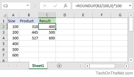
For example in cell C2, you can use the IF function and the ROUNDUP function as follows:

=ROUNDUP(B2/100,0)*100

This will return the correct value of 400 for a value of 318 in cell B2. Just copy this formula to cell C3, C4 and so on.

Источник

The IF function runs a logical test and returns one value for a TRUE result, and another value for a FALSE result. The result from IF can be a value, a cell reference, or even another formula. By combining the IF function with other logical functions like AND and OR, you can test more than one condition at a time.

Syntax

The generic syntax for the IF function looks like this:

=IF(logical_test,[value_if_true],[value_if_false])

The first argument, logical_test, is typically an expression that returns either TRUE or FALSE. The second argument, value_if_true, is the value to return when logical_test is TRUE. The last argument, value_if_false, is the value to return when logical_test is FALSE. Both value_if_true and value_if_false are optional, but you must provide one or the other. For example, if cell A1 contains 80, then:

=IF(A1>75,TRUE) // returns TRUE
=IF(A1>75,"OK") // returns "OK"
=IF(A1>85,"OK") // returns FALSE
=IF(A1>75,10,0) // returns 10
=IF(A1>85,10,0) // returns 0
=IF(A1>75,"Yes","No") // returns "Yes"
=IF(A1>85,"Yes","No") // returns "No"

Notice that text values like «OK», «Yes», «No», etc. must be enclosed in double quotes («»). However, numeric values should not be enclosed in quotes.

Logical tests

The IF function supports logical operators (>,<,<>,=) when creating logical tests. Most commonly, the logical_test in IF is a complete logical expression that will evaluate to TRUE or FALSE. The table below shows some common examples:

Goal	Logical test
If A1 is greater than 75	A1>75
If A1 equals 100	A1=100
If A1 is less than or equal to 100	A1<=100
If A1 equals «Red»	A1=»red»
If A1 is not equal to «Red»	A1<>»red»
If A1 is less than B1	A1<B1
If A1 is empty	A1=»»
If A1 is not empty	A1<>»»
If A1 is less than current date	A1<TODAY()

Notice text values must be enclosed in double quotes («»), but numbers do not. The IF function does not support wildcards, but you can combine IF with COUNTIF to get basic wildcard functionality. To test for substrings in a cell, you can use the IF function with the SEARCH function.

Pass or Fail example

In the worksheet shown above, we want to assign either «Pass» or «Fail» based on a test score. A passing score is 70 or higher. The formula in D6, copied down, is:

=IF(C5>=70,"Pass","Fail")

Translation: If the value in C5 is greater than or equal to 70, return «Pass». Otherwise, return «Fail».

Note that the logical flow of this formula can be reversed. This formula returns the same result:

=IF(C5<70,"Fail","Pass")

Translation: If the value in C5 is less than 70, return «Fail». Otherwise, return «Pass».

Both formulas above, when copied down, will return correct results.

Note: If you are new to the idea of formula criteria, this article explains many examples.

Assign points based on color

In the worksheet below, we want to assign points based on the color in column B. If the color is «red», the result should be 100. If the color is «blue», the result should be 125. This requires that we use a formula based on two IF functions, one nested inside the other. The formula in C5, copied down, is:

=IF(B5="red",100,IF(B5="blue",125))

Translation: IF the value in B5 is «red», return 100. Else, if the value in B5 is «blue», return 125.

There are three things to notice in this example:

The formula will return FALSE if the value in B5 is anything except «red» or «blue»
The text values «red» and «blue» must be enclosed in double quotes («»)
The IF function is not case-sensitive and will match «red», «Red», «RED», or «rEd».

This is a simple example of a nested IFs formula. See below for a more complex example.

Return another formula

The IF function can return another formula as a result. For example, the formula below will return A1*5% when A1 is less than 100, and A1*7% when A1 is greater than or equal to 100:

=IF(A1<100,A1*5%,A1*7%)

Nested IF statements

The IF function can be «nested». A «nested IF» refers to a formula where at least one IF function is nested inside another in order to test for more conditions and return more possible results. Each IF statement needs to be carefully «nested» inside another so that the logic is correct. For example, the following formula can be used to assign a grade rather than a pass / fail result:

=IF(C6<70,"F",IF(C6<75,"D",IF(C6<85,"C",IF(C6<95,"B","A"))))

Up to 64 IF functions can be nested. However, in general, you should consider other functions, like VLOOKUP or XLOOKUP for more complex scenarios, because they can handle more conditions in a more streamlined fashion. For a more details see this article on nested IFs.

Note: the newer IFS function is designed to handle multiple conditions without nesting. However, a lookup function like VLOOKUP or XLOOKUP is usually a better approach unless the logic for each condition is custom.

IF with AND, OR, NOT

The IF function can be combined with the AND function and the OR function. For example, to return «OK» when A1 is between 7 and 10, you can use a formula like this:

=IF(AND(A1>7,A1<10),"OK","")

Translation: if A1 is greater than 7 and less than 10, return «OK». Otherwise, return nothing («»).

To return B1+10 when A1 is «red» or «blue» you can use the OR function like this:

=IF(OR(A1="red",A1="blue"),B1+10,B1)

Translation: if A1 is red or blue, return B1+10, otherwise return B1.

=IF(NOT(A1="red"),B1+10,B1)

Translation: if A1 is NOT red, return B1+10, otherwise return B1.

IF cell contains specific text

Because the IF function does not support wildcards, it is not obvious how to configure IF to check for a specific substring in a cell. A common approach is to combine the ISNUMBER function and the SEARCH function to create a logical test like this:

=ISNUMBER(SEARCH(substring,A1)) // returns TRUE or FALSE

For example, to check for the substring «xyz» in cell A1, you can use a formula like this:

=IF(ISNUMBER(SEARCH("xyz",A1)),"Yes","No")

Read a detailed explanation here.

More information

Read more about nested IFs
Learn how to use VLOOKUP instead of nested IFs (video)
50 Examples of formula criteria

Notes

The IF function is not case-sensitive.
To count values conditionally, use the COUNTIF or the COUNTIFS functions.
To sum values conditionally, use the SUMIF or the SUMIFS functions.
If any of the arguments to IF are supplied as arrays, the IF function will evaluate every element of the array.

Источник

Excel IF AND OR functions on their own aren’t very exciting, but mix them up with the IF Statement and you’ve got yourself a formula that’s much more powerful.

In this tutorial we’re going to take a look at the basics of the AND and OR functions and then put them to work with an IF Statement. If you aren’t familiar with IF Statements, click here to read that tutorial first.

IF Formula Builder

Our IF Formula Builder does the hard work of creating IF formulas.

You just need to enter a few pieces of information, and the workbook creates the formula for you.

AND Function

The AND function belongs to the logic family of formulas, along with IF, OR and a few others. It’s useful when you have multiple conditions that must be met.

In Excel language on its own the AND formula reads like this:

=AND(logical1,[logical2]....)

Now to translate into English:

=AND(is condition 1 true, AND condition 2 true (add more conditions if you want)

OR Function

The OR function is useful when you are happy if one, OR another condition is met.

In Excel language on its own the OR formula reads like this:

=OR(logical1,[logical2]....)

Now to translate into English:

=OR(is condition 1 true, OR condition 2 true (add more conditions if you want)

See, I did say they weren’t very exciting, but let’s mix them up with IF and put AND and OR to work.

IF AND Formula

First let’s set the scene of our challenge for the IF, AND formula:

In our spreadsheet below we want to calculate a bonus to pay the children’s TV personalities listed. The rules, as devised by my 4 year old son, are:

1) If the TV personality is Popular AND

2) If they earn less than $100k per year they get a 10% bonus (my 4 year old will write them an IOU, he’s good for it though).

In cell D2 we will enter our IF AND formula as follows:

In English first

=IF(Spider Man is Popular, AND he earns <$100k),  calculate his salary x 10%, if not put "Nil" in the cell)

Now in Excel’s language:

=IF(AND(B2="Yes",C2<100),C2x$H$1,"Nil")

You’ll notice that the two conditions are typed in first, and then the outcomes are entered. You can have more than two conditions; in fact you can have up to 30 by simply separating each condition with a comma (see warning below about going overboard with this though).

IF OR Formula

Again let’s set the scene of our challenge for the IF, OR formula:

The revised rules, as devised by my 4 year old son, are:

1) If the TV personality is Popular OR

2) If they earn less than $100k per year they get a 10% bonus.

In cell D2 we will enter our IF OR formula as follows:

In English first

=IF(Spider Man is Popular, OR he earns <$100k), calculate his salary x 10%, if not put “Nil” in the cell)

Now in Excel’s language:

=IF(OR(B2="Yes",C2<100),C2x$H$1,"Nil")

Notice how a subtle change from the AND function to the OR function has a significant impact on the bonus figure.

Just like the AND function, you can have up to 30 OR conditions nested in the one formula, again just separate each condition with a comma.

Try other operators

You can set your conditions to test for specific text, as I have done in this example with B2=»Yes», just put the text you want to check between inverted comas “ ”.

Alternatively you can test for a number and because the AND and OR functions belong to the logic family, you can employ different tests other than the less than (<) operator used in the examples above.

Other operators you could use are:

= Equal to
> Greater Than
<= Less than or equal to
>= Greater than or equal to
<> Less than or greater than

Warning: Don’t go overboard with nesting IF, AND, and OR’s, as it will be painful to decipher if you or someone else ever needs to update the formula in months or years to come.

Note: These formulas work in all versions of Excel, however versions pre Excel 2007 are limited to 7 nested IF’s.

Download the Workbook

Enter your email address below to download the sample workbook.

By submitting your email address you agree that we can email you our Excel newsletter.

Excel IF AND OR Practice Questions

IF AND Formula Practice

In the embedded Excel workbook below insert a formula (in the grey cells in column E), that returns the text ‘Yes’, when a product SKU should be reordered, based on the following criteria:

If Stock on hand is less than 20,000 AND
Demand level is ‘High’

If the above conditions are met, return ‘Yes’, otherwise, return ‘No’.

Tips for working with the embedded workbook:

Use arrow keys to move around the worksheet when you can’t click on the cells with your mouse
Use shortcut keys CTRL+C to copy and CTRL+V to paste
Don’t forget to absolute cell references where applicable
Do not enter anything in column F
Double click to edit a cell
Refresh the page to reset the embedded workbook

IF OR Formula Practice

In the embedded Excel workbook below insert a formula (in the grey cells in column E) that calculates the bonus due for each salesperson. A $500 bonus is paid if a salesperson meets either target in cells C24 and C25, otherwise they earn $0 bonus.

Want More Excel Formulas

Why not visit our list of Excel formulas. You’ll find a huge range all explained in plain English, plus PivotTables and other Excel tools and tricks. Enjoy 🙂

Источник

Simple IF examples

Common problems

Need more help?

See Also

Need more help?

Что возвращает функция

Синтаксис

Аргументы функции

Дополнительная информация

Функция Если в Excel примеры с несколькими условиями

Пример 1. Проверяем простое числовое условие с помощью функции IF (ЕСЛИ)

Пример 2. Использование вложенной функции IF (ЕСЛИ) для проверки условия выражения

Пример 3. Вычисляем сумму комиссии с продаж с помощью функции IF (ЕСЛИ) в Excel

Пример 4. Используем логические операторы (AND/OR) (И/ИЛИ) в функции IF (ЕСЛИ) в Excel

Пример 5. Преобразуем ошибки в значения “0” с помощью функции IF (ЕСЛИ)

Description

Syntax

Parameters or Arguments

Returns

Example (as Worksheet Function)

Combining the IF function with Other Logical Functions

AND function

OR function

Frequently Asked Questions

Syntax

Logical tests

Pass or Fail example

Assign points based on color

Return another formula

Nested IF statements

IF with AND, OR, NOT

IF cell contains specific text

More information

Notes

IF Formula Builder

AND Function

OR Function

IF AND Formula

IF OR Formula

Download the Workbook

Excel IF AND OR Practice Questions

IF AND Formula Practice

IF OR Formula Practice

Want More Excel Formulas