Excel add cell to text - Word и Excel - помощь в работе с программами

Welcome back to another Excel #formulafriday blog. Today I want to share with you a nice handy Excel tip using a well-known formula. Let’s learn how to insert the contents of an Excel cell into a sentence. This is a really great way to save time if you use the same report every week or month. All you really need to do is update the report with the latest figures!.

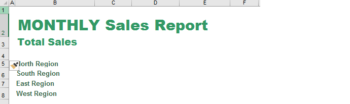
Let’s walk through an example of my Monthly Sales Report. Every month I report on Sales Per Region, the standard format is the same every month and the only thing that changes is a handful of cells. Let’s free up some time and get this report a little more automated using the CONCATENATE Function.

Using The CONCATENATE Function.

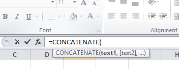
The syntax of this formula is

=CONCATENATE(TEXT1,TEXT2…)

Up to 255 text entries can be added to the function and each one of them should be separated by a comma.

One point to note, CONCATENATE does NOT add in extra spaces between text, in order to do this, you need to accommodate these extra spaces within the formula. Let’s take a look at an example.

Right, let’s get back to the extract from my report-

Next, all I need to do is combine the text in cells B5:B8 with my monthly sales figures which are automatically updated on the datasheet of my Monthly Sales Report. You can be see these in the screenshot below. My sales figures I want to always refer to in the specified area of my Sales Report are contained in cells C6:C9.

As you have probably noticed we have some formatting on our cells that contain our sales figures for the previous month. So, I need to take into account this formatting for the sales report to not only look good but be easily interpreted.

Let’s get on with some formula fun.

First, we take CONCATENATE which simply combines two or more text strings into one. After that, we just need to separate the text strings with commas.

Building The Formula.

Let’s start with the Northern Region. We have three text strings as even space is classed as a separate text string. We also have to just ensure we force the formatting on the value sales from our data area of the Sale Report.

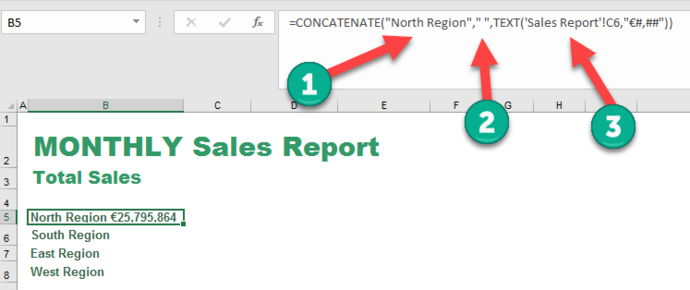
For the last argument (3) in the formula, we use the TEXT function, which takes two arguments. Firstly, it takes the Value (which we take from our data area of the sales report). We can then declare which formatting we want to use. I just need to hit enter to complete the process.

Now we have the formula set up. I just update the data area of my sales report. That’s all that I need to do. Excel automatically populates the presentation part of my Monthly Sales Report.

What Next? Want More Excel Tips?

If you want more Excel and VBA tips then sign up for my Monthly Newsletter where I share 3 Tips on the first Wednesday of the month and receive my free Ebook, 30 Excel Tips.

If you want to see all of the blog posts in the Formula Friday series. Click on the link below

How To Excel At Excel – Formula Friday Blog Posts.

Источник

Combine text from two or more cells into one cell

You can combine data from multiple cells into a single cell using the Ampersand symbol (&) or the CONCAT function.

Combine data with the Ampersand symbol (&)

Select the cell where you want to put the combined data.
Type = and select the first cell you want to combine.
Type & and use quotation marks with a space enclosed.
Select the next cell you want to combine and press enter. An example formula might be =A2&» «&B2.

Combine data using the CONCAT function

Select the cell where you want to put the combined data.
Type =CONCAT(.
Select the cell you want to combine first.

Use commas to separate the cells you are combining and use quotation marks to add spaces, commas, or other text.
Close the formula with a parenthesis and press Enter. An example formula might be =CONCAT(A2, » Family»).

Need more help?

Method 1: Using the ampersand Operator

An ampersand (&) can be used to easily combine text strings in Excel. Let’s see how you use it to add text at the beginning or end or both in Excel.

Using the ampersand Operator to Add Text to the Beginning of all Cells

The ampersand (&) is an operator that is mainly used to join several text strings into one.

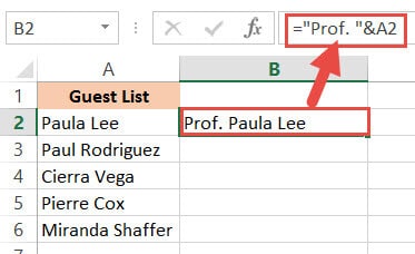
Here’s how you can use it to add text to the beginning of all cells in a range. Let us assume you have the following list of names and want to add the title “Prof.” before every name:

Below are the steps to add a text before a text string in Excel:

Click on the first cell of the column where you want the converted names to appear (B2).
Type equal sign (=), followed by the text “Prof. “, followed by an ampersand (&).
Select the cell containing the first name (A2).
Press the Return Key.
You will notice that the title “Prof.” is added before the first name in the list.
It’s now time to copy this formula to the rest of the cells in the column. Simply double click the fill handle (located at the bottom right of cell B2). Alternatively, you can drag down the fill handle to achieve the same effect.

That’s it, all your cells in column B should now contain the title “Prof.” preceding each name.

Using the ampersand Operator to Add Text to the End of all Cells

Now let us see how to add some text to the end of every name in the dataset. Let us say you want to add the text “(MD)” at the end of every name. In that case, here are the steps you need to follow:

Click on the first cell of the column where you want the converted names to appear (C2 in our case).
Type equal sign (=)
Select the cell containing the first name (B2 in our case).
Next, insert an ampersand (&), followed by the text “ (MD)”.
Press the Return Key.
You will notice that the text “(MD).” added after the first name in the list.
It’s now time to copy this formula to the rest of the cells in the column. Simply double click the fill handle (located at the bottom right of cell C2). Alternatively, you can drag down the fill handle to achieve the same effect.

All your cells in column C should now contain the text “(MD”) at the end of each name.

Adding text before and after a text string

Method 2: Using the CONCATENATE Function

CONCATENATE is an Excel function that you can use to add text at the beginning and end of the text string.

Let’s see how to use CONCATENATE to do this.

Using CONCATENATE to Add Text to the Beginning of all Cells

The CONCATENATE() function provides the same functionality as the ampersand (&) operator. The only difference is in the way both are used.

The general syntax for the CONCATENATE function is:

=CONCATENATE(text1, [text2], …)

Where text1, text2, etc. are substrings that you want to combine together.

Let’s apply the CONCATENATE function to the same dataset as above:

Click on the first cell of the column where you want the converted names to appear (B2).
Type equal sign (=).
Enter the function CONCATENATE, followed by an opening bracket (.
Type the title “Prof. ” in double-quotes, followed by a comma (,).
Select the cell containing the first name (A2)
Place a closing bracket. In our example, your formula should now be: =CONCATENATE(“Prof. “,A2).
Press the Return Key.
You will notice that the title “Prof.” is added before the first name on the list.
It’s now time to copy this formula to the rest of the cells in the column. Simply double click the fill handle (located at the bottom right of cell B2). Alternatively, you can drag down the fill handle to achieve the same effect.

That’s it, all your cells in column B should now contain the title “Prof.” preceding each name.

Using CONCATENATE to Add Text to the End of all Cells

Click on the first cell of the column where you want the converted names to appear (C2 in our example).
Type equal sign (=).
Enter the function CONCATENATE, followed by an opening bracket (.
Select the cell containing the first name (B2 in our example).
Next, insert a comma, followed by the text “ (MD)”.
Place a closing bracket. In our example, your formula should now be: =CONCATENATE(B2,” (MD)”).
Press the Return Key.
You will notice that the text “(MD).” added after the first name in the list.
It’s now time to copy this formula to the rest of the cells in the column. Simply double click the fill handle (located at the bottom right of cell C2).

All your cells in column C should now contain the text “(MD”) at the end of each name.

Notice that since you’re using a formula, your column C depends on columns A and B. So if you make any changes to the original values in column A, they get reflected in column C.

If you decide to only retain the converted names and delete columns A and B, you will get an error, as shown below:

Issue when deleting rhe dependent columns

To make sure that this does not happen, it’s best to first convert the formula results to permanent values copying them and pasting them as values in the same column (Right-click and select Paste Options->Values from the Popup menu).

Now you can go ahead and delete columns A and B if you need to.

Also read: How to Remove First Character in Excel?

Method 3: Using the Flash Fill Feature

Flash fill is a relatively new feature that looks at the pattern of what you are trying to achieve and then does it for all the cells in a column.

You can also use Flash fill to so text manipulation as we will see in the following examples.

Using Flash Fill to Add Text to the Beginning of all Cells

The Excel flash fill feature is like a magical button. It is available if you’re on any Excel version from 2013 onwards.

The feature takes advantage of Excel’s pattern recognition capabilities. It basically recognizes a pattern in your data and automatically fills in the other cells of the column with the same pattern for you.

Here’s how you can use Flash Fill to add text to the beginning of all cells in a column:

Click on the first cell of the column where you want the converted names to appear (B2).
Manually type in the text Prof. , followed by the first name of your list.
Press the Return Key.
Click on cell B2 again.
Under the Data tab, click on the Flash Fill button (in the ‘Data Tools’ group). Alternatively, you can just press CTRL+E on your keyboard (Command+E if you’re on a Mac).

This will copy the same pattern to the rest of the cells in the column… in a flash!

Using Flash Fill to Add Text to the End of all Cells in a Column

If you want to add the text “ (MD)” to the end of the names, follow the same steps:

Click on the first cell of the column where you want the converted names to appear (C2).
Manually type in or copy the text from column B2 into C2.
Add the text “(MD)” after that.
Under the Data tab, click on the Flash Fill or press CTRL+E on your keyboard (Command+E if you’re on a Mac).

That’s all, you get every cell filled in with the same pattern!

We especially like this method because it is simple, quick, and easy. Moreover, since it’s formula-free, the results do not depend on the original columns.

So they remain unchanged even if you delete rows A and B!

Result in case you delete all the other columns

Method 4: Using VBA Code

And of course, if you’re comfortable with VBA, you can also add text before or after a text string using it.

Using VBA to Add Text to the Beginning of all Cells in a Column

If coding with VBA does not intimidate you then this method can help get your work done quickly too.

Here’s the code we will be using to add the title “Prof. “ to the beginning of all cells in a range. You can select and copy it:

Sub add_text_to_beginning()
Dim rng As Range
Dim cell As Range
Set rng = Application.Selection
For Each cell In rng
cell.Offset(0, 1).Value = "Prof. " & cell.Value
Next cell
End Sub

Follow these steps to use the above code:

From the Developer Menu Ribbon, select Visual Basic.
Once your VBA window opens, Click Insert->Module. Now you can start coding. Type or copy-paste the above lines of code into the module window. Your code is now ready to run.
Select the range of cells containing the text you want to convert. Make sure the column next to it is blank because this is where the code will display the results.
Navigate to Developer->Macros-> add_text_to_beginning->Run.

You will now see the converted text next to your selected range of cells.

Note: You can change the text in line 6 from “Prof. ” to whatever text you need to add to the beginning of all cells.

Using VBA to Add Text to the End of all Cells in a Column

Now, what if you want to add text to the end of all the cells, instead of the beginning? This only involves making a tweak to line 6 of the above code. So if you want to add the text “ (MD)” to the end of all cells, change line 6 to:

cell.Offset(0, 1).Value = cell.Value & “ (MD)”

So your full code should now be:

Sub add_text_to_end()
Dim rng As Range
Dim cell As Range
Set rng = Application.Selection
For Each cell In rng
cell.Offset(0, 1).Value = cell.Value & " (MD)"
Next cell
End Sub

Here’s the final result:

You can now delete the first two columns if you need to. Do remember to keep a backup of your sheet, because the results of VBA code are usually irreversible.

Note: You can change the text in line 6 from “ (MD)” to whatever text you need to add to the end of all cells in the range.

In this tutorial, we showed you four ways in which you can add text to the beginning and/ or end of all cells in a range.

There are plenty of other methods that you can find online too, and all of them work just as well as the ones shown here.

You may feel free to choose whatever method suits you, your requirement, and your version of Excel. In the end, what matters is getting what you need to be done quickly and effectively.

Other Excel tutorials you may like:

How to Remove Text after a Specific Character in Excel
How to Reverse a Text String in Excel
How to Count How Many Times a Word Appears in Excel
How to Remove Commas in Excel (from Numbers or Text String)
How to Remove a Specific Character from a String in Excel
How to Change Uppercase to Lowercase in Excel
How to Separate Address in Excel?
How to Concatenate with Line Breaks in Excel?
How to Separate Names in Excel

Источник

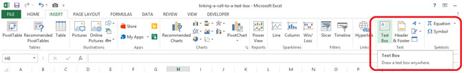
Microsoft Excel has a functionality where we can link a textbox to a specific cell. If we change the data in the cell, the value of the linked cell gets updated automatically. Below are the following steps to link a cell to a text box:

1. Open Excel
2. Click on the Insert tab
3. Click the Text Box button

4. A text Box will Open

5. Select the Text Box
6. Type = in the Formula Bar
7. Select the cell where you want to give a reference

Let us take an example

1. Open Excel
2. Click on the Insert tab
3. Click the Text Box button
4. A text Box will Open
5. Select the Text Box
6. Type = in the Formula Bar
7. Select the cell A1

8. After we select Cell A1, automatically it will display “=$A$1”
9. Now when we change the Text in cell A1, automatically text in the Text Box will change

Источник

Using The CONCATENATE Function.

Building The Formula.

What Next? Want More Excel Tips?

If you want more Excel and VBA tips then sign up for my Monthly Newsletter where I share 3 Tips on the first Wednesday of the month and receive my free Ebook, 30 Excel Tips.

If you want to see all of the blog posts in the Formula Friday series. Click on the link below

Combine data with the Ampersand symbol (&)

Combine data using the CONCAT function

Need more help?

See also

Need more help?

Method 1: Using the ampersand Operator

Using the ampersand Operator to Add Text to the Beginning of all Cells

Using the ampersand Operator to Add Text to the End of all Cells

Method 2: Using the CONCATENATE Function

Using CONCATENATE to Add Text to the Beginning of all Cells

Using CONCATENATE to Add Text to the End of all Cells

Method 3: Using the Flash Fill Feature

Using Flash Fill to Add Text to the Beginning of all Cells

Using Flash Fill to Add Text to the End of all Cells in a Column

Method 4: Using VBA Code

Using VBA to Add Text to the Beginning of all Cells in a Column

Using VBA to Add Text to the End of all Cells in a Column