Excel activate cell if

IF function

The IF function is one of the most popular functions in Excel, and it allows you to make logical comparisons between a value and what you expect.

So an IF statement can have two results. The first result is if your comparison is True, the second if your comparison is False.

For example, =IF(C2=”Yes”,1,2) says IF(C2 = Yes, then return a 1, otherwise return a 2).

Use the IF function, one of the logical functions, to return one value if a condition is true and another value if it’s false.

IF(logical_test, value_if_true, [value_if_false])

For example:

• =IF(A2>B2,»Over Budget»,»OK»)

• =IF(A2=B2,B4-A4,»»)

Argument name	Description
logical_test    (required)	The condition you want to test.
value_if_true    (required)	The value that you want returned if the result of logical_test is TRUE.
value_if_false    (optional)	The value that you want returned if the result of logical_test is FALSE.

Simple IF examples

• =IF(C2=”Yes”,1,2)

In the above example, cell D2 says: IF(C2 = Yes, then return a 1, otherwise return a 2)

• =IF(C2=1,”Yes”,”No”)

In this example, the formula in cell D2 says: IF(C2 = 1, then return Yes, otherwise return No)As you see, the IF function can be used to evaluate both text and values. It can also be used to evaluate errors. You are not limited to only checking if one thing is equal to another and returning a single result, you can also use mathematical operators and perform additional calculations depending on your criteria. You can also nest multiple IF functions together in order to perform multiple comparisons.

• =IF(C2>B2,”Over Budget”,”Within Budget”)

In the above example, the IF function in D2 is saying IF(C2 Is Greater Than B2, then return “Over Budget”, otherwise return “Within Budget”)

• =IF(C2>B2,C2-B2,0)

In the above illustration, instead of returning a text result, we are going to return a mathematical calculation. So the formula in E2 is saying IF(Actual is Greater than Budgeted, then Subtract the Budgeted amount from the Actual amount, otherwise return nothing).

• =IF(E7=”Yes”,F5*0.0825,0)

In this example, the formula in F7 is saying IF(E7 = “Yes”, then calculate the Total Amount in F5 * 8.25%, otherwise no Sales Tax is due so return 0)

Note: If you are going to use text in formulas, you need to wrap the text in quotes (e.g. “Text”). The only exception to that is using TRUE or FALSE, which Excel automatically understands.

Common problems

Problem	What went wrong
0 (zero) in cell	There was no argument for either value_if_true or value_if_False arguments. To see the right value returned, add argument text to the two arguments, or add TRUE or FALSE to the argument.
#NAME? in cell	This usually means that the formula is misspelled.

Need more help?

You can always ask an expert in the Excel Tech Community or get support in the Answers community.

See Also

IF function — nested formulas and avoiding pitfalls

IFS function

Using IF with AND, OR and NOT functions

COUNTIF function

How to avoid broken formulas

Overview of formulas in Excel

Свойство ActiveCell объекта Application, применяемое в VBA для возвращения активной ячейки, расположенной на активном листе в окне приложения Excel.

Свойство ActiveCell объекта Application возвращает объект Range, представляющий активную ячейку на активном листе в активном или указанном окне приложения Excel. Если окно не отображает лист, применение свойства Application.ActiveCell приведет к ошибке.

Если свойство ActiveCell применяется к активному окну приложения Excel, то идентификатор объекта (Application или ActiveWindow) можно в коде VBA Excel не указывать. Следующие выражения, скопированные с сайта разработчиков, являются эквивалентными:

ActiveCell Application.ActiveCell ActiveWindow.ActiveCell Application.ActiveWindow.ActiveCell

Но если нам необходимо возвратить активную ячейку, находящуюся в неактивном окне приложения Excel, тогда без указания идентификатора объекта на обойтись:

Sub Primer1()     With Windows(«Книга2.xlsx»)         .ActiveCell = 325         MsgBox .ActiveCell.Address         MsgBox .ActiveCell.Value     End With End Sub

Программно сделать ячейку активной в VBA Excel можно с помощью методов Activate и Select.

Различие методов Activate и Select

Выберем программно диапазон «B2:E6» методом Select и выведем адрес активной ячейки:

Sub Primer2()     Range(«B2:E6»).Select     ActiveCell = ActiveCell.Address End Sub

Результат:

Как видим, активной стала первая ячейка выбранного диапазона, расположенная слева вверху. Если мы поменяем местами границы диапазона (Range("E6:B2").Select), все равно активной станет та же первая ячейка.

Теперь сделаем активной ячейку «D4», расположенную внутри выделенного диапазона, с помощью метода Activate:

Sub Primer3()     Range(«E6:B2»).Select     Range(«D4»).Activate     ActiveCell = ActiveCell.Address End Sub

Результат:

Как видим, выбранный диапазон не изменился, а активная ячейка переместилась из первой ячейки выделенного диапазона в ячейку «D4».

И, наконец, выберем ячейку «D4», расположенную внутри выделенного диапазона, с помощью метода Select:

Sub Primer4()     Range(«E6:B2»).Select     Range(«D4»).Select     ActiveCell = ActiveCell.Address End Sub

Результат:

Как видим, ранее выбранный диапазон был заменен новым, состоящим из одной ячейки «D4». Такой же результат будет и при активации ячейки, расположенной вне выбранного диапазона, методом Activate:

Sub Primer5()     Range(«E6:B2»).Select     Range(«A3»).Activate     ActiveCell = ActiveCell.Address End Sub

Аналогично ведут себя методы Activate и Select при работе с выделенной группой рабочих листов.

Свойство Application.ActiveCell используется для обращения к одной ячейке, являющейся активной, а для работы со всеми ячейками выделенного диапазона используется свойство Application.Selection.

---

Всё о работе с ячейками в Excel-VBA: обращение, перебор, удаление, вставка, скрытие, смена имени.

Содержание:

Table of Contents:

• Что такое ячейка Excel?
• Способы обращения к ячейкам
  • Выбор и активация
  • Получение и изменение значений ячеек
    • Ячейки открытой книги
    • Ячейки закрытой книги 
  • Перебор ячеек
  • Перебор в произвольном диапазоне
• Свойства и методы ячеек
  • Имя ячейки
  • Адрес ячейки
  • Размеры ячейки
• Запуск макроса активацией ячейки

2 нюанса:

1. Я почти везде стараюсь использовать ThisWorkbook (а не, например, ActiveWorkbook) для обращения к текущей книге, в которой написан этот код (считаю это наиболее безопасным для новичков способом обращения к книгам, чтобы случайно не внести изменения в другие книги). Для экспериментов можете вставлять этот код в модули, коды книги, либо листа, и он будет работать только в пределах этой книги. 
2. Я использую английский эксель и у меня по стандарту листы называются Sheet1, Sheet2 и т.д. Если вы работаете в русском экселе, то замените Thisworkbook.Sheets(«Sheet1») на Thisworkbook.Sheets(«Лист1»). Если этого не сделать, то вы получите ошибку в связи с тем, что пытаетесь обратиться к несуществующему объекту. Можно также заменить на Thisworkbook.Sheets(1), но это менее безопасно.

Что такое ячейка Excel?

В большинстве мест пишут: «элемент, образованный пересечением столбца и строки». Это определение полезно для людей, которые не знакомы с понятием «таблица». Для того, чтобы понять чем на самом деле является ячейка Excel, необходимо заглянуть в объектную модель Excel. При этом определения объектов «ряд», «столбец» и «ячейка» будут отличаться в зависимости от того, как мы работаем с файлом.

Объекты в Excel-VBA. Пока мы работаем в Excel без углубления в VBA определение ячейки как «пересечения» строк и столбцов нам вполне хватает, но если мы решаем как-то автоматизировать процесс в VBA, то о нём лучше забыть и просто воспринимать лист как «мешок» ячеек, с каждой из которых VBA позволяет работать как минимум тремя способами:

1. по цифровым координатам (ряд, столбец),
2. по адресам формата А1, B2 и т.д. (сценарий целесообразности данного способа обращения в VBA мне сложно представить)
3. по уникальному имени (во втором и третьем вариантах мы будем иметь дело не совсем с ячейкой, а с объектом VBA range, который может состоять из одной или нескольких ячеек). Функции и методы объектов Cells и Range отличаются. Новичкам я бы порекомендовал работать с ячейками VBA только с помощью Cells и по их цифровым координатам и использовать Range только по необходимости.

Все три способа обращения описаны далее

Как это хранится на диске и как с этим работать вне Excel? С точки зрения хранения и обработки вне Excel и VBA. Сделать это можно, например, сменив расширение файла с .xls(x) на .zip и открыв этот архив.

Пример содержимого файла Excel:

Далее xl -> worksheets и мы видим файл листа

Содержимое файла:

 То же, но более наглядно:

<?xml version="1.0" encoding="UTF-8" standalone="yes"?>
<worksheet xmlns="http://schemas.openxmlformats.org/spreadsheetml/2006/main" xmlns:r="http://schemas.openxmlformats.org/officeDocument/2006/relationships" xmlns:mc="http://schemas.openxmlformats.org/markup-compatibility/2006" mc:Ignorable="x14ac xr xr2 xr3" xmlns:x14ac="http://schemas.microsoft.com/office/spreadsheetml/2009/9/ac" xmlns:xr="http://schemas.microsoft.com/office/spreadsheetml/2014/revision" xmlns:xr2="http://schemas.microsoft.com/office/spreadsheetml/2015/revision2" xmlns:xr3="http://schemas.microsoft.com/office/spreadsheetml/2016/revision3" xr:uid="{00000000-0001-0000-0000-000000000000}">
	<dimension ref="B2:F6"/>
	<sheetViews>
		<sheetView tabSelected="1" workbookViewId="0">
			<selection activeCell="D12" sqref="D12"/>
		</sheetView>
	</sheetViews>
	<sheetFormatPr defaultRowHeight="14.4" x14ac:dyDescent="0.3"/>
	<sheetData>
		<row r="2" spans="2:6" x14ac:dyDescent="0.3">
			<c r="B2" t="s">
				<v>0</v>
			</c>
		</row>
		<row r="3" spans="2:6" x14ac:dyDescent="0.3">
			<c r="C3" t="s">
				<v>1</v>
			</c>
		</row>
		<row r="4" spans="2:6" x14ac:dyDescent="0.3">
			<c r="D4" t="s">
				<v>2</v>
			</c>
		</row>
		<row r="5" spans="2:6" x14ac:dyDescent="0.3">
			<c r="E5" t="s">
				<v>0</v></c>
		</row>
		<row r="6" spans="2:6" x14ac:dyDescent="0.3">
			<c r="F6" t="s"><v>3</v>
		</c></row>
	</sheetData>
	<pageMargins left="0.7" right="0.7" top="0.75" bottom="0.75" header="0.3" footer="0.3"/>
</worksheet>

Как мы видим, в структуре объектной модели нет никаких «пересечений». Строго говоря рабочая книга — это архив структурированных данных в формате XML. При этом в каждую «строку» входит «столбец», и в нём в свою очередь прописан номер значения данного столбца, по которому оно подтягивается из другого XML файла при открытии книги для экономии места за счёт отсутствия повторяющихся значений. Почему это важно. Если мы захотим написать какой-то обработчик таких файлов, который будет напрямую редактировать данные в этих XML, то ориентироваться надо на такую модель и структуру данных. И правильное определение будет примерно таким: ячейка — это объект внутри столбца, который в свою очередь находится внутри строки в файле xml, в котором хранятся данные о содержимом листа.

Способы обращения к ячейкам

Выбор и активация

Почти во всех случаях можно и стоит избегать использования методов Select и Activate. На это есть две причины:

1. Это лишь имитация действий пользователя, которая замедляет выполнение программы. Работать с объектами книги можно напрямую без использования методов Select и Activate.
2. Это усложняет код и может приводить к неожиданным последствиям. Каждый раз перед использованием Select необходимо помнить, какие ещё объекты были выбраны до этого и не забывать при необходимости снимать выбор. Либо, например, в случае использования метода Select в самом начале программы может быть выбрано два листа вместо одного потому что пользователь запустил программу, выбрав другой лист.

Можно выбирать и активировать книги, листы, ячейки, фигуры, диаграммы, срезы, таблицы и т.д.

Отменить выбор  ячеек можно методом Unselect:

Selection.Unselect

Отличие выбора от активации — активировать можно только один объект из раннее выбранных. Выбрать можно несколько объектов.

Если вы записали и редактируете код макроса, то лучше всего заменить Select и Activate на конструкцию With … End With. Например, предположим, что мы записали вот такой макрос:

Sub Macro1()
' Macro1 Macro
    Range("F4:F10,H6:H10").Select 'выбрали два несмежных диапазона зажав ctrl
    Range("H6").Activate          'показывает только то, что я начал выбирать второй диапазон с этой ячейки (она осталась белой). Это действие ни на что не влияет
    With Selection.Interior       
        .Pattern = xlSolid
        .PatternColorIndex = xlAutomatic
        .Color = 65535            'залили желтым цветом, нажав на кнопку заливки на верхней панели
        .TintAndShade = 0
        .PatternTintAndShade = 0
    End With
End Sub

Почему макрос записался таким неэффективным образом? Потому что в каждый момент времени (в каждой строке) программа не знает, что вы будете делать дальше. Поэтому в записи выбор ячеек и действия с ними — это два отдельных действия. Этот код лучше всего оптимизировать (особенно если вы хотите скопировать его внутрь какого-нибудь цикла, который должен будет исполняться много раз и перебирать много объектов). Например, так:

Sub Macro11()
'
' Macro1 Macro
    Range("F4:F10,H6:H10").Select '1. смотрим, что за объект выбран (что идёт до .Select)
    Range("H6").Activate
    With Selection.Interior       '2. понимаем, что у выбранного объекта есть свойство interior, с которым далее идёт работа
        .Pattern = xlSolid
        .PatternColorIndex = xlAutomatic
        .Color = 65535
        .TintAndShade = 0
        .PatternTintAndShade = 0
    End With
End Sub



Sub Optimized_Macro()
    With Range("F4:F10,H6:H10").Interior '3. переносим объект напрямую в конструкцию With вместо Selection
' ////// Здесь я для надёжности прописал бы ещё Thisworkbook.Sheet("ИмяЛиста") перед Range,
' ////// чтобы минимизировать риск любых случайных изменений других листов и книг
' ////// With Thisworkbook.Sheet("ИмяЛиста").Range("F4:F10,H6:H10").Interior
        .Pattern = xlSolid               '4. полностью копируем всё, что было записано рекордером внутрь блока with
        .PatternColorIndex = xlAutomatic
        .Color = 55555                   '5. здесь я поменял цвет на зеленый, чтобы было видно, работает ли код при поочерёдном запуске двух макросов
        .TintAndShade = 0
        .PatternTintAndShade = 0
    End With
End Sub

Пример сценария, когда использование Select и Activate оправдано:

Допустим, мы хотим, чтобы во время исполнения программы мы одновременно изменяли несколько листов одним действием и пользователь видел какой-то определённый лист. Это можно сделать примерно так:

Sub Select_Activate_is_OK()
Thisworkbook.Worksheets(Array("Sheet1", "Sheet3")).Select 'Выбираем несколько листов по именам
Thisworkbook.Worksheets("Sheet3").Activate 'Показываем пользователю третий лист
'Далее все действия с выбранными ячейками через Select будут одновременно вносить изменения в оба выбранных листа

'Допустим, что тут мы решили покрасить те же два диапазона:
Range("F4:F10,H6:H10").Select
    Range("H6").Activate
    With Selection.Interior       
        .Pattern = xlSolid
        .PatternColorIndex = xlAutomatic
        .Color = 65535
        .TintAndShade = 0
        .PatternTintAndShade = 0
    End With

End Sub

Единственной причиной использовать этот код по моему мнению может быть желание зачем-то показать пользователю определённую страницу книги в какой-то момент исполнения программы. С точки зрения обработки объектов, опять же, эти действия лишние.

Получение и изменение значений ячеек

Значение ячеек можно получать/изменять с помощью свойства value. 

'Если нужно прочитать / записать значение ячейки, то используется свойство Value
a = ThisWorkbook.Sheets("Sheet1").Cells (1,1).Value 'записать значение ячейки А1 листа "Sheet1" в переменную "a"
ThisWorkbook.Sheets("Sheet1").Cells (1,1).Value = 1  'задать значение ячейки А1 (первый ряд, первый столбец) листа "Sheet1"

'Если нужно прочитать текст как есть (с форматированием), то можно использовать свойство .text:
ThisWorkbook.Sheets("Sheet1").Cells (1,1).Text = "1" 
a = ThisWorkbook.Sheets("Sheet1").Cells (1,1).Text

'Когда проявится разница:
'Например, если мы считываем дату в формате "31 декабря 2021 г.", хранящуюся как дата
a = ThisWorkbook.Sheets("Sheet1").Cells (1,1).Value 'эапишет как "31.12.2021"
a = ThisWorkbook.Sheets("Sheet1").Cells (1,1).Text  'запишет как "31 декабря 2021 г."

Ячейки открытой книги

К ячейкам можно обращаться:

'В книге, в которой хранится макрос (на каком-то из листов, либо в отдельном модуле или форме)
ThisWorkbook.Sheets("Sheet1").Cells(1,1).Value        'По номерам строки и столбца
ThisWorkbook.Sheets("Sheet1").Cells(1,"A").Value      'По номерам строки и букве столбца
ThisWorkbook.Sheets("Sheet1").Range("A1").Value       'По адресу - вариант 1
ThisWorkbook.Sheets("Sheet1").[A1].Value              'По адресу - вариант 2
ThisWorkbook.Sheets("Sheet1").Range("CellName").Value 'По имени ячейки (для этого ей предварительно нужно его присвоить)

'Те же действия, но с использованием полного названия рабочей книги (книга должна быть открыта)
Workbooks("workbook.xlsm").Sheets("Sheet1").Cells(1,1).Value 'По номерам строки и столбца
Workbooks("workbook.xlsm").Sheets("Sheet1").Cells(1,"A").Value                'По номерам строки и букве столбца
Workbooks("workbook.xlsm").Sheets("Sheet1").Range("A1").Value                 'По адресу - вариант 1
Workbooks("workbook.xlsm").Sheets("Sheet1").[A1].Value                        'По адресу - вариант 2
Workbooks("workbook.xlsm").Sheets("Sheet1").Range("CellName").Value           'По имени ячейки (для этого ей предварительно нужно его присвоить)

Ячейки закрытой книги

Если нужно достать или изменить данные в другой закрытой книге, то необходимо прописать открытие и закрытие книги. Непосредственно работать с закрытой книгой не получится, потому что данные в ней хранятся отдельно от структуры и при открытии Excel каждый раз производит расстановку значений по соответствующим «слотам» в структуре. Подробнее о том, как хранятся данные в xlsx см выше.

Workbooks.Open Filename:="С:closed_workbook.xlsx"    'открыть книгу (она становится активной)
a = ActiveWorkbook.Sheets("Sheet1").Cells(1,1).Value  'достать значение ячейки 1,1
ActiveWorkbook.Close False                            'закрыть книгу (False => без сохранения)

Скачать пример, в котором можно посмотреть, как доставать и как записывать значения в закрытую книгу. 

Код из файла:

Option Explicit
Sub get_value_from_closed_wb() 'достать значение из закрытой книги
Dim a, wb_path, wsh As String
wb_path = ThisWorkbook.Sheets("Sheet1").Cells(2, 3).Value 'get path to workbook from sheet1
wsh = ThisWorkbook.Sheets("Sheet1").Cells(3, 3).Value
Workbooks.Open Filename:=wb_path
a = ActiveWorkbook.Sheets(wsh).Cells(3, 3).Value
ActiveWorkbook.Close False
ThisWorkbook.Sheets("Sheet1").Cells(4, 3).Value = a
End Sub

Sub record_value_to_closed_wb() 'записать значение в закрытую книгу
Dim wb_path, b, wsh As String
wsh = ThisWorkbook.Sheets("Sheet1").Cells(3, 3).Value
wb_path = ThisWorkbook.Sheets("Sheet1").Cells(2, 3).Value 'get path to workbook from sheet1
b = ThisWorkbook.Sheets("Sheet1").Cells(5, 3).Value 'get value to record in the target workbook
Workbooks.Open Filename:=wb_path
ActiveWorkbook.Sheets(wsh).Cells(4, 4).Value = b 'add new value to cell D4 of the target workbook
ActiveWorkbook.Close True
End Sub

Перебор ячеек

Перебор в произвольном диапазоне

Скачать файл со всеми примерами

Пройтись по всем ячейкам в нужном диапазоне можно разными способами. Основные:

1. Цикл For Each. Пример:

   Sub iterate_over_cells()
   
   For Each c In ThisWorkbook.Sheets("Sheet1").Range("B2:D4").Cells
   MsgBox (c)
   Next c
   
   End Sub​

   Этот цикл выведет в виде сообщений значения ячеек в диапазоне B2:D4 по порядку по строкам слева направо и по столбцам — сверху вниз. Данный способ можно использовать для действий, в который вам не важны номера ячеек (закрашивание, изменение форматирования, пересчёт чего-то и т.д.).

2. Ту же задачу можно решить с помощью двух вложенных циклов — внешний будет перебирать ряды, а вложенный — ячейки в рядах. Этот способ я использую чаще всего, потому что он позволяет получить больше контроля над исполнением: на каждой итерации цикла нам доступны координаты ячеек. Для перебора всех ячеек на листе этим методом потребуется найти последнюю заполненную ячейку. Пример кода:

   Sub iterate_over_cells()
   
   Dim cl, rw As Integer
   Dim x As Variant
   
   'перебор области 3x3
   For rw = 1 To 3 ' цикл для перебора рядов 1-3
   
       For cl = 1 To 3 'цикл для перебора столбцов 1-3
           x = ThisWorkbook.Sheets("Sheet1").Cells(rw + 1, cl + 1).Value
           MsgBox (x)
       Next cl
   Next rw
   
   
   
   'перебор всех ячеек на листе. Последняя ячейка определена с помощью UsedRange
   'LastRow = ActiveSheet.UsedRange.Row + ActiveSheet.UsedRange.Rows.Count - 1
   'LastCol = ActiveSheet.UsedRange.Column + ActiveSheet.UsedRange.Columns.Count - 1
   'For rw = 1 To LastRow 'цикл перебора всех рядов
   '    For cl = 1 To LastCol 'цикл для перебора всех столбцов
   '        Действия 
   '    Next cl
   'Next rw
   
   
   End Sub​

3. Если нужно перебрать все ячейки в выделенном диапазоне на активном листе, то код будет выглядеть так:

   Sub iterate_cell_by_cell_over_selection()
       Dim ActSheet As Worksheet
       Dim SelRange As Range
       Dim cell As Range
       
    
       Set ActSheet = ActiveSheet
       Set SelRange = Selection
       
       'if we want to do it in every cell of the selected range
       For Each cell In Selection
       MsgBox (cell.Value)
       
       Next cell
   
   End Sub​

   Данный метод подходит для интерактивных макросов, которые выполняют действия над выбранными пользователем областями.

4. Перебор ячеек в ряду

   Sub iterate_cells_in_row()
       Dim i, RowNum, StartCell As Long
       
       RowNum = 3 'какой ряд
       StartCell = 0 ' номер начальной ячейки (минус 1, т.к. в цикле мы прибавляем i)
       
       For i = 1 To 10 ' 10 ячеек в выбранном ряду
       ThisWorkbook.Sheets("Sheet1").Cells(RowNum, i + StartCell).Value = i '(i + StartCell) добавляет 1 к номеру столбца при каждом повторении
       Next i
   
   End Sub

5. Перебор ячеек в столбце

   Sub iterate_cells_in_column()
       Dim i, ColNum, StartCell As Long
       
       ColNum = 3 'какой столбец
       StartCell = 0 ' номер начальной ячейки (минус 1, т.к. в цикле мы прибавляем i)
       
       For i = 1 To 10 ' 10 ячеек
       ThisWorkbook.Sheets("Sheet1").Cells(i + StartCell, ColNum).Value = i ' (i + StartCell) добавляет 1 к номеру ряда при каждом повторении
       Next i
   
   End Sub​

Свойства и методы ячеек

Имя ячейки

Присвоить новое имя можно так:

Thisworkbook.Sheets(1).Cells(1,1).name = "Новое_Имя"

Для того, чтобы сменить имя ячейки нужно сначала удалить существующее имя, а затем присвоить новое. Удалить имя можно так:

ActiveWorkbook.Names("Старое_Имя").Delete

Пример кода для переименования ячеек:

Sub rename_cell()

old_name = "Cell_Old_Name"
new_name = "Cell_New_Name"

ActiveWorkbook.Names(old_name).Delete
ThisWorkbook.Sheets(1).Cells(2, 1).Name = new_name
End Sub

Sub rename_cell_reverse()

old_name = "Cell_New_Name"
new_name = "Cell_Old_Name"

ActiveWorkbook.Names(old_name).Delete
ThisWorkbook.Sheets(1).Cells(2, 1).Name = new_name
End Sub

Адрес ячейки

Sub get_cell_address() ' вывести адрес ячейки в формате буква столбца, номер ряда
  '$A$1 style
  txt_address = ThisWorkbook.Sheets(1).Cells(3, 2).Address
  MsgBox (txt_address)
End Sub

Sub get_cell_address_R1C1()' получить адрес столбца в формате номер ряда, номер столбца
  'R1C1 style
  txt_address = ThisWorkbook.Sheets(1).Cells(3, 2).Address(ReferenceStyle:=xlR1C1)
  MsgBox (txt_address)
End Sub

  'пример функции, которая принимает 2 аргумента: название именованного диапазона и тип желаемого адреса 
  '(1- тип $A$1 2- R1C1 - номер ряда, столбца)
Function get_cell_address_by_name(str As String, address_type As Integer)
  '$A$1 style
  Select Case address_type
    Case 1
      txt_address = Range(str).Address
    Case 2
      txt_address = Range(str).Address(ReferenceStyle:=xlR1C1)
    Case Else
      txt_address = "Wrong address type selected. 1,2 available"
    End Select
  get_cell_address_by_name = txt_address
End Function

'перед запуском нужно убедиться, что в книге есть диапазон с названием, 
'адрес которого мы хотим получить, иначе будет ошибка
Sub test_function() 'запустите эту программу, чтобы увидеть, как работает функция
  x = get_cell_address_by_name("MyValue", 2)
  MsgBox (x)
End Sub

Размеры ячейки

Ширина и длина ячейки в VBA меняется, например, так:

Sub change_size()
Dim x, y As Integer
Dim w, h As Double

'получить координаты целевой ячейки
x = ThisWorkbook.Sheets("Sheet1").Cells(2, 2).Value
y = ThisWorkbook.Sheets("Sheet1").Cells(3, 2).Value

'получить желаемую ширину и высоту ячейки
w = ThisWorkbook.Sheets("Sheet1").Cells(6, 2).Value
h = ThisWorkbook.Sheets("Sheet1").Cells(7, 2).Value

'сменить высоту и ширину ячейки с координатами x,y
ThisWorkbook.Sheets("Sheet1").Cells(x, y).RowHeight = h
ThisWorkbook.Sheets("Sheet1").Cells(x, y).ColumnWidth = w


End Sub

Прочитать значения ширины и высоты ячеек можно двумя способами (однако результаты будут в разных единицах измерения). Если написать просто Cells(x,y).Width или Cells(x,y).Height, то будет получен результат в pt (привязка к размеру шрифта). 

Sub get_size()
Dim x, y As Integer
'получить координаты ячейки, с которой мы будем работать
x = ThisWorkbook.Sheets("Sheet1").Cells(2, 2).Value
y = ThisWorkbook.Sheets("Sheet1").Cells(3, 2).Value

'получить длину и ширину выбранной ячейки в тех же единицах измерения, в которых мы их задавали
ThisWorkbook.Sheets("Sheet1").Cells(2, 6).Value = ThisWorkbook.Sheets("Sheet1").Cells(x, y).ColumnWidth
ThisWorkbook.Sheets("Sheet1").Cells(3, 6).Value = ThisWorkbook.Sheets("Sheet1").Cells(x, y).RowHeight

'получить длину и ширину с помощью свойств ячейки (только для чтения) в поинтах (pt)
ThisWorkbook.Sheets("Sheet1").Cells(7, 9).Value = ThisWorkbook.Sheets("Sheet1").Cells(x, y).Width
ThisWorkbook.Sheets("Sheet1").Cells(8, 9).Value = ThisWorkbook.Sheets("Sheet1").Cells(x, y).Height

End Sub

Скачать файл с примерами изменения и чтения размера ячеек

Запуск макроса активацией ячейки

Для запуска кода VBA при активации ячейки необходимо вставить в код листа нечто подобное:

3 важных момента, чтобы это работало:

1. Этот код должен быть вставлен в код листа (здесь контролируется диапазон D4)

2-3. Программа, ответственная за запуск кода при выборе ячейки, должна называться Worksheet_SelectionChange и должна принимать значение переменной Target, относящейся к триггеру SelectionChange. Другие доступные триггеры можно посмотреть в правом верхнем углу (2).

Скачать файл с базовым примером (как на картинке)

Скачать файл с расширенным примером (код ниже)

Option Explicit

Private Sub Worksheet_SelectionChange(ByVal Target As Range)

        ' имеем в виду, что триггер SelectionChange будет запускать эту Sub после каждого клика мышью (после каждого клика будет проверяться:
          '1. количество выделенных ячеек и 
          '2. не пересекается ли выбранный диапазон с заданным в этой программе диапазоном.
        ' поэтому в эту программу не стоит без необходимости писать никаких других тяжелых операций

    If Selection.Count = 1 Then 'запускаем программу только если выбрано не более 1 ячейки


    'вариант модификации - брать адрес ячейки из другой ячейки:
    'Dim CellName as String
    'CellName = Activesheet.Cells(1,1).value 'брать текстовое имя контролируемой ячейки из A1 (должно быть в формате Буква столбца + номер строки)
    'If Not Intersect(Range(CellName), Target) Is Nothing Then
    'для работы этой модификации следующую строку надо закомментировать/удалить



        If Not Intersect(Range("D4"), Target) Is Nothing Then 
        'если заданный (D4) и выбранный диапазон пересекаются 
        '(пересечение диапазонов НЕ равно Nothing)

        'можно прописать диапазон из нескольких ячеек:
        'If Not Intersect(Range("D4:E10"), Target) Is Nothing Then
        'можно прописать несколько диапазонов:
        'If Not Intersect(Range("D4:E10"), Target) Is Nothing or Not Intersect(Range("A4:A10"), Target) Is Nothing Then

            Call program 'выполняем программу
        End If
    End If
End Sub

Sub program()

MsgBox ("Program Is running") 'здесь пишем код того, что произойдёт при выборе нужной ячейки


End Sub

This Excel tutorial explains how to use the Excel IF function with syntax and examples.

Description

The Microsoft Excel IF function returns one value if the condition is TRUE, or another value if the condition is FALSE.

The IF function is a built-in function in Excel that is categorized as a Logical Function. It can be used as a worksheet function (WS) in Excel. As a worksheet function, the IF function can be entered as part of a formula in a cell of a worksheet.

Subscribe

---

If you want to follow along with this tutorial, download the example spreadsheet.

Download Example

Syntax

The syntax for the IF function in Microsoft Excel is:

IF( condition, value_if_true, [value_if_false] )

Parameters or Arguments

condition

The value that you want to test.

value_if_true

It is the value that is returned if condition evaluates to TRUE.

value_if_false

Optional. It is the value that is returned if condition evaluates to FALSE.

Returns

The IF function returns value_if_true when the condition is TRUE.
The IF function returns value_if_false when the condition is FALSE.
The IF function returns FALSE if the value_if_false parameter is omitted and the condition is FALSE.

Example (as Worksheet Function)

Let’s explore how to use the IF function as a worksheet function in Microsoft Excel.

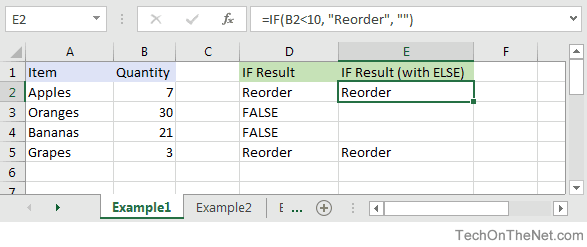
Based on the Excel spreadsheet above, the following IF examples would return:

=IF(B2<10, "Reorder", "")
Result: "Reorder"

=IF(A2="Apples", "Equal", "Not Equal")
Result: "Equal"

=IF(B3>=20, 12, 0)
Result: 12

Combining the IF function with Other Logical Functions

Quite often, you will need to specify more complex conditions when writing your formula in Excel. You can combine the IF function with other logical functions such as AND, OR, etc. Let’s explore this further.

AND function

The IF function can be combined with the AND function to allow you to test for multiple conditions. When using the AND function, all conditions within the AND function must be TRUE for the condition to be met. This comes in very handy in Excel formulas.

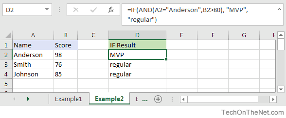
Based on the spreadsheet above, you can combine the IF function with the AND function as follows:

=IF(AND(A2="Anderson",B2>80), "MVP", "regular")
Result: "MVP"

=IF(AND(B2>=80,B2<=100), "Great Score", "Not Bad")
Result: "Great Score"

=IF(AND(B3>=80,B3<=100), "Great Score", "Not Bad")
Result: "Not Bad"

=IF(AND(A2="Anderson",A3="Smith",A4="Johnson"), 100, 50)
Result: 100

=IF(AND(A2="Anderson",A3="Smith",A4="Parker"), 100, 50)
Result: 50

In the examples above, all conditions within the AND function must be TRUE for the condition to be met.

OR function

The IF function can be combined with the OR function to allow you to test for multiple conditions. But in this case, only one or more of the conditions within the OR function needs to be TRUE for the condition to be met.

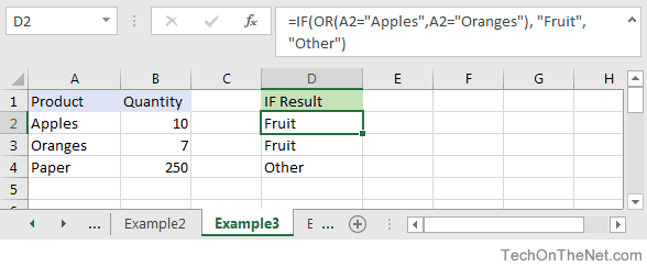
Based on the spreadsheet above, you can combine the IF function with the OR function as follows:

=IF(OR(A2="Apples",A2="Oranges"), "Fruit", "Other")
Result: "Fruit"

=IF(OR(A4="Apples",A4="Oranges"),"Fruit","Other")
Result: "Other"

=IF(OR(A4="Bananas",B4>=100), 999, "N/A")
Result: 999

=IF(OR(A2="Apples",A3="Apples",A4="Apples"), "Fruit", "Other")
Result: "Fruit"

In the examples above, only one of the conditions within the OR function must be TRUE for the condition to be met.

Let’s take a look at one more example that involves ranges of percentages.

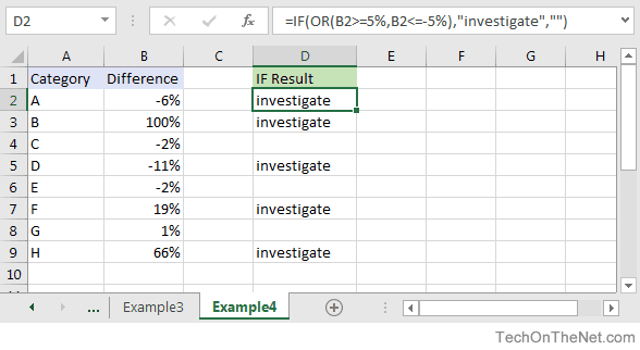
Based on the spreadsheet above, we would have the following formula in cell D2:

=IF(OR(B2>=5%,B2<=-5%),"investigate","")
Result: "investigate"

This IF function would return «investigate» if the value in cell B2 was either below -5% or above 5%. Since -6% is below -5%, it will return «investigate» as the result. We have copied this formula into cells D3 through D9 to show you the results that would be returned.

For example, in cell D3, we would have the following formula:

=IF(OR(B3>=5%,B3<=-5%),"investigate","")
Result: "investigate"

This formula would also return «investigate» but this time, it is because the value in cell B3 is greater than 5%.

Frequently Asked Questions

Question: In Microsoft Excel, I’d like to use the IF function to create the following logic:

if C11>=620, and C10=»F»or»S», and C4<=$1,000,000, and C4<=$500,000, and C7<=85%, and C8<=90%, and C12<=50, and C14<=2, and C15=»OO», and C16=»N», and C19<=48, and C21=»Y», then reference cell A148 on Sheet2. Otherwise, return an empty string.

Answer: The following formula would accomplish what you are trying to do:

=IF(AND(C11>=620, OR(C10="F",C10="S"), C4<=1000000, C4<=500000, C7<=0.85, C8<=0.9, C12<=50, C14<=2, C15="OO", C16="N", C19<=48, C21="Y"), Sheet2!A148, "")

---

Question: In Microsoft Excel, I’m trying to use the IF function to return 0 if cell A1 is either < 150,000 or > 250,000. Otherwise, it should return A1.

Answer: You can use the OR function to perform an OR condition in the IF function as follows:

=IF(OR(A1<150000,A1>250000),0,A1)

In this example, the formula will return 0 if cell A1 was either less than 150,000 or greater than 250,000. Otherwise, it will return the value in cell A1.

---

Question: In Microsoft Excel, I’m trying to use the IF function to return 25 if cell A1 > 100 and cell B1 < 200. Otherwise, it should return 0.

Answer: You can use the AND function to perform an AND condition in the IF function as follows:

=IF(AND(A1>100,B1<200),25,0)

In this example, the formula will return 25 if cell A1 is greater than 100 and cell B1 is less than 200. Otherwise, it will return 0.

---

Question: In Microsoft Excel, I need to write a formula that works this way:

IF (cell A1) is less than 20, then times it by 1,
IF it is greater than or equal to 20 but less than 50, then times it by 2
IF its is greater than or equal to 50 and less than 100, then times it by 3
And if it is great or equal to than 100, then times it by 4

Answer: You can write a nested IF statement to handle this. For example:

=IF(A1<20, A1*1, IF(A1<50, A1*2, IF(A1<100, A1*3, A1*4)))

---

Question: In Microsoft Excel, I need a formula in cell C5 that does the following:

IF A1+B1 <= 4, return $20
IF A1+B1 > 4 but <= 9, return $35
IF A1+B1 > 9 but <= 14, return $50
IF A1+B1 >= 15, return $75

Answer: In cell C5, you can write a nested IF statement that uses the AND function as follows:

=IF((A1+B1)<=4,20,IF(AND((A1+B1)>4,(A1+B1)<=9),35,IF(AND((A1+B1)>9,(A1+B1)<=14),50,75)))

---

Question: In Microsoft Excel, I need a formula that does the following:

IF the value in cell A1 is BLANK, then return «BLANK»
IF the value in cell A1 is TEXT, then return «TEXT»
IF the value in cell A1 is NUMERIC, then return «NUM»

Answer: You can write a nested IF statement that uses the ISBLANK function, the ISTEXT function, and the ISNUMBER function as follows:

=IF(ISBLANK(A1)=TRUE,"BLANK",IF(ISTEXT(A1)=TRUE,"TEXT",IF(ISNUMBER(A1)=TRUE,"NUM","")))

---

Question: In Microsoft Excel, I want to write a formula for the following logic:

IF R1<0.3 AND R2<0.3 AND R3<0.42 THEN «OK» OTHERWISE «NOT OK»

Answer: You can write an IF statement that uses the AND function as follows:

=IF(AND(R1<0.3,R2<0.3,R3<0.42),"OK","NOT OK")

---

Question: In Microsoft Excel, I need a formula for the following:

IF cell A1= PRADIP then value will be 100
IF cell A1= PRAVIN then value will be 200
IF cell A1= PARTHA then value will be 300
IF cell A1= PAVAN then value will be 400

Answer: You can write an IF statement as follows:

=IF(A1="PRADIP",100,IF(A1="PRAVIN",200,IF(A1="PARTHA",300,IF(A1="PAVAN",400,""))))

---

Question: In Microsoft Excel, I want to calculate following using an «if» formula:

if A1<100,000 then A1*.1% but minimum 25
and if A1>1,000,000 then A1*.01% but maximum 5000

Answer: You can write a nested IF statement that uses the MAX function and the MIN function as follows:

=IF(A1<100000,MAX(25,A1*0.1%),IF(A1>1000000,MIN(5000,A1*0.01%),""))

---

Question: In Microsoft Excel, I am trying to create an IF statement that will repopulate the data from a particular cell if the data from the formula in the current cell equals 0. Below is my attempt at creating an IF statement that would populate the data; however, I was unsuccessful.

=IF(IF(ISERROR(M24+((L24-S24)/AA24)),"0",M24+((L24-S24)/AA24)))=0,L24)

The initial part of the formula calculates the EAC (Estimate At completion = AC+(BAC-EV)/CPI); however if the current EV (Earned Value) is zero, the EAC will equal zero. IF the outcome is zero, I would like the BAC (Budget At Completion), currently recorded in another cell (L24), to be repopulated in the current cell as the EAC.

Answer: You can write an IF statement that uses the OR function and the ISERROR function as follows:

=IF(OR(S24=0,ISERROR(M24+((L24-S24)/AA24))),L24,M24+((L24-S24)/AA24))

---

Question: I have been looking at your Excel IF, AND and OR sections and found this very helpful, however I cannot find the right way to write a formula to express if C2 is either 1,2,3,4,5,6,7,8,9 and F2 is F and F3 is either D,F,B,L,R,C then give a value of 1 if not then 0. I have tried many formulas but just can’t get it right, can you help please?

Answer: You can write an IF statement that uses the AND function and the OR function as follows:

=IF(AND(C2>=1,C2<=9, F2="F",OR(F3="D",F3="F",F3="B",F3="L",F3="R",F3="C")),1,0)

---

Question:In Excel, I have a roadspeed of a car in m/s in cell A1 and a drop down menu of different units in C1 (which unclude mph and kmh). I have used the following IF function in B1 to convert the number to the unit selected from the dropdown box:

=IF(C1="mph","=A1*2.23693629",IF(C1="kmh","A1*3.6"))

However say if kmh was selected B1 literally just shows A1*3.6 and does not actually calculate it. Is there away to get it to calculate it instead of just showing the text message?

Answer: You are very close with your formula. Because you are performing mathematical operations (such as A1*2.23693629 and A1*3.6), you do not need to surround the mathematical formulas in quotes. Quotes are necessary when you are evaluating strings, not performing math.

Try the following:

=IF(C1="mph",A1*2.23693629,IF(C1="kmh",A1*3.6))

---

Question:For an IF statement in Excel, I want to combine text and a value.

For example, I want to put an equation for work hours and pay. IF I am paid more than I should be, I want it to read how many hours I owe my boss. But if I work more than I am paid for, I want it to read what my boss owes me (hours*Pay per Hour).

I tried the following:

=IF(A2<0,"I owe boss" abs(A2) "Hours","Boss owes me" abs(A2)*15 "dollars")

Is it possible or do I have to do it in 2 separate cells? (one for text and one for the value)

Answer: There are two ways that you can concatenate text and values. The first is by using the & character to concatenate:

=IF(A2<0,"I owe boss " & ABS(A2) & " Hours","Boss owes me " & ABS(A2)*15 &  " dollars")

Or the second method is to use the CONCATENATE function:

=IF(A2<0,CONCATENATE("I owe boss ", ABS(A2)," Hours"), CONCATENATE("Boss owes me ", ABS(A2)*15,  " dollars"))

---

Question:I have Excel 2000. IF cell A2 is greater than or equal to 0 then add to C1. IF cell B2 is greater than or equal to 0 then subtract from C1. IF both A2 and B2 are blank then equals C1. Can you help me with the IF function on this one?

Answer: You can write a nested IF statement that uses the AND function and the ISBLANK function as follows:

=IF(AND(ISBLANK(A2)=FALSE,A2>=0),C1+A2, IF(AND(ISBLANK(B2)=FALSE,B2>=0),C1-B2, IF(AND(ISBLANK(A2)=TRUE, ISBLANK(B2)=TRUE),C1,"")))

---

Question:How would I write this equation in Excel? IF D12<=0 then D12*L12, IF D12 is > 0 but <=600 then D12*F12, IF D12 is >600 then ((600*F12)+((D12-600)*E12))

Answer: You can write a nested IF statement as follows:

=IF(D12<=0,D12*L12,IF(D12>600,((600*F12)+((D12-600)*E12)),D12*F12))

---

Question:In Excel, I have this formula currently:

=IF(OR(A1>=40, B1>=40, C1>=40), "20", (A1+B1+C1)-20)

If one of my salesman does sale for $40-$49, then his commission is $20; however if his/her sale is less (for example $35) then the commission is that amount minus $20 ($35-$20=$15). I have 3 columns that are needed based on the type of sale. Only one column per row will be needed. The problem is that, when left blank, the total in the formula cell is -20. I need help setting up this formula so that when the 3 columns are left blank, the cell with the formula is left blank as well.

Answer: Using the AND function and the ISBLANK function, you can write your IF statement as follows:

=IF(AND(ISBLANK(A1),ISBLANK(B1),ISBLANK(C1)),"",IF(OR(A1>40, B1>40, C1>40), "20", (A1+B1+C1)-20))

In this formula, we are using the ISBLANK function to check if all 3 cells A1, B1, and C1 are blank, and if they are return a blank value («»). Then the rest is the formula that you originally wrote.

---

Question:In Excel, I need to create a simple booking and and out system, that shows a date out and a date back

«A1» = allows person to input date booked out
«A2» =allows person to input date booked back in

«A3″= shows status of product, eg, booked out, overdue return etc.

I can automate A3 with the following IF function:

=IF(ISBLANK(A2),"booked out","returned")

But what I cant get to work is if the product is out for 10 days or more, I would like the cell to say «send email»

Can you assist?

Answer: Using the TODAY function and adding an additional IF function, you can write your formula as follows:

=IF(ISBLANK(A2),IF(TODAY()-A1>10,"send email","booked out"),"returned")

---

Question:Using Microsoft Excel, I need a formula in cell U2 that does the following:

IF the date in E2<=12/31/2010, return T2*0.75
IF the date in E2>12/31/2010 but <=12/31/2011, return T2*0.5
IF the date in E2>12/31/2011, return T2*0

I tried using the following formula, but it gives me «#VALUE!»

=IF(E2<=DATE(2010,12,31),T2*0.75), IF(AND(E2>DATE(2010,12,31),E2<=DATE(2011,12,31)),T2*0.5,T2*0)

Can someone please help? Thanks.

Answer: You were very close…you just need to adjust your parentheses as follows:

=IF(E2<=DATE(2010,12,31),T2*0.75, IF(AND(E2>DATE(2010,12,31),E2<=DATE(2011,12,31)),T2*0.5,T2*0))

---

Question:In Excel, I would like to add 60 days if grade is ‘A’, 45 days if grade is ‘B’ and 30 days if grade is ‘C’. It would roughly look something like this, but I’m struggling with commas, brackets, etc.

(IF C5=A)=DATE(YEAR(B5)+0,MONTH(B5)+0,DAY(B5)+60),
(IF C5=B)=DATE(YEAR(B5)+0,MONTH(B5)+0,DAY(B5)+45),
(IF C5=C)=DATE(YEAR(B5)+0,MONTH(B5)+0,DAY(B5)+30)

Answer:You should be able to achieve your date calculations with the following formula:

=IF(C5="A",B5+60,IF(C5="B",B5+45,IF(C5="C",B5+30)))

---

Question:In Excel, I am trying to write a function and can’t seem to figure it out. Could you help?

IF D3 is < 31, then 1.51
IF D3 is between 31-90, then 3.40
IF D3 is between 91-120, then 4.60
IF D3 is > 121, then 5.44

Answer:You can write your formula as follows:

=IF(D3>121,5.44,IF(D3>=91,4.6,IF(D3>=31,3.4,1.51)))

---

Question:I would like ask a question regarding the IF statement. How would I write in Excel this problem?

I have to check if cell A1 is empty and if not, check if the value is less than equal to 5. Then multiply the amount entered in cell A1 by .60. The answer will be displayed on Cell A2.

Answer:You can write your formula in cell A2 using the IF function and ISBLANK function as follows:

=IF(AND(ISBLANK(A1)=FALSE,A1<=5),A1*0.6,"")

---

Question:In Excel, I’m trying to nest an OR command and I can’t find the proper way to write it. I want the spreadsheet to do the following:

If D6 equals «HOUSE» and C6 equals either «MOUSE» or «CAT», I want to return the value in cell B6. Otherwise, the formula should return the value «BLANK».

I tried the following:

=IF((D6="HOUSE")*(C6="MOUSE")*OR(C6="CAT"));B6;"BLANK")

If I only ask for HOUSE and MOUSE or HOUSE and CAT, it works, but as soon as I ask for MOUSE OR CAT, it doesn’t work.

Answer:You can write your formula using the AND function and OR function as follows:

=IF(AND(D6="HOUSE",OR(C6="MOUSE",C6="CAT")),B6,"BLANK")

This will return the value in B6 if D6 equals «HOUSE» and C6 equals either «MOUSE» or «CAT». If those conditions are not met, the formula will return the text value of «BLANK».

---

Question:In Microsoft Excel, I’m trying to write the following formula:

If cell A1 equals «jaipur», «udaipur» or «jodhpur», then cell A2 should display «rajasthan»
If cell A1 equals «bangalore», «mysore» or «belgum», then cell A2 should display «karnataka»

Please help.

Answer:You can write your formula using the OR function as follows:

=IF(OR(A1="jaipur",A1="udaipur",A1="jodhpur"),"rajasthan", IF(OR(A1="bangalore",A1="mysore",A1="belgum"),"karnataka"))

This will return «rajasthan» if A1 equals either «jaipur», «udaipur» or «jodhpur» and it will return «karnataka» if A1 equals either «bangalore», «mysore» or «belgum».

---

Question:In Microsoft Excel I’m trying to achieve the following with IF function:

If a value in any cell in column F is «food» then add the value of its corresponding cell in column G (eg a corresponding cell for F3 is G3). The IF function is performed in another cell altogether. I can do it for a single pair of cells but I don’t know how to do it for an entire column. Could you help?

At the moment, I’ve got this:

=IF(F3="food"; G3; 0)

Answer:This formula can be created using the SUMIF formula instead of using the IF function:

=SUMIF(F1:F10,"=food",G1:G10)

This will evaluate the first 10 rows of data in your spreadsheet. You may need to adjust the ranges accordingly.

I notice that you separate your parameters with semi-colons, so you might need to replace the commas in the formula above with semi-colons.

---

Question:I’m looking for an Exel formula that says:

If F3 is «H» and E3 is «H», return 1
If F3 is «A» and E3 is «A», return 2
If F3 is «d» and E3 is «d», return 3

Appreciate if you can help.

Answer:This Excel formula can be created using the AND formula in combination with the IF function:

=IF(AND(F3="H",E3="H"),1,IF(AND(F3="A",E3="A"),2,IF(AND(F3="d",E3="d"),3,"")))

We’ve defaulted the formula to return a blank if none of the conditions above are met.

---

Question:I am trying to get Excel to check different boxes and check if there is text/numbers listed in the cells and then spit out «Complete» if all 5 Boxes have text/Numbers or «Not Complete» if one or more is empty. This is what I have so far and it doesn’t work.

=IF(OR(ISBLANK(J2),ISBLANK(M2),ISBLANK(R2),ISBLANK (AA2),ISBLANK (AB2)),"Not Complete","")

Answer:First, you are correct in using the ISBLANK function, however, you have a space between ISBLANK and (AA2), as well as ISBLANK and (AB2). This might seem insignificant, but Excel can be very picky and will return a #NAME? error. So first you need to eliminate those spaces.

Next, you need to change the ELSE condition of your IF function to return «Complete».

You should be able to modify your formula as follows:

=IF(OR(ISBLANK(J2),ISBLANK(M2),ISBLANK(R2),ISBLANK(AA2),ISBLANK(AB2)), "Not Complete", "Complete")

Now if any of the cell J2, M2, R2, AA2, or AB2 are blank, the formula will return «Not Complete». If all 5 cells have a value, the formula will return «Complete».

---

Question:I’m very new to the Excel world, and I’m trying to figure out how to set up the proper formula for an If/then cell.

What I’m trying for is:

If B2’s value is 1 to 5, then multiply E2 by .77
If B2’s value is 6 to 10, then multiply E2 by .735
If B2’s value is 11 to 19, then multiply E2 by .7
If B2’s value is 20 to 29, then multiply E2 by .675
If B2’s value is 30 to 39, then multiply E2 by .65

I’ve tried a few different things thinking I was on the right track based on the IF, and AND function tutorials here, but I can’t seem to get it right.

Answer:To write your IF formula, you need to nest multiple IF functions together in combination with the AND function.

The following formula should work for what you are trying to do:

=IF(AND(B2>=1, B2<=5), E2*0.77, IF(AND(B2>=6, B2<=10), E2*0.735, IF(AND(B2>=11, B2<=19), E2*0.7, IF(AND(B2>=20, B2<=29), E2*0.675, IF(AND(B2>=30, B2<=39), E2*0.65,"")))))

As one final component of your formula, you need to decide what to do when none of the conditions are met. In this example, we have returned «» when the value in B2 does not meet any of the IF conditions above.

---

Question:Here is the Excel formula that has me between a rock and a hard place.

If E45 <= 50, return 44.55
If E45 > 50 and E45 < 100, return 42
If E45 >=200, return 39.6

Again thank you very much.

Answer:You should be able to write this Excel formula using a combination of the IF function and the AND function.

The following formula should work:

=IF(E45<=50, 44.55, IF(AND(E45>50, E45<100), 42, IF(E45>=200, 39.6, "")))

Please note that if none of the conditions are met, the Excel formula will return «» as the result.

---

Question:I have a nesting OR function problem:

My nonworking formula is:

=IF(C9=1,K9/J7,IF(C9=2,K9/J7,IF(C9=3,K9/L7,IF(C9=4,0,K9/N7))))

In Cell C9, I can have an input of 1, 2, 3, 4 or 0. The problem is on how to write the «or» condition when a «4 or 0» exists in Column C. If the «4 or 0» conditions exists in Column C I want Column K divided by Column N and the answer to be placed in Column M and associated row

Answer:You should be able to use the OR function within your IF function to test for C9=4 OR C9=0 as follows:

=IF(C9=1,K9/J7,IF(C9=2,K9/J7,IF(C9=3,K9/L7,IF(OR(C9=4,C9=0),K9/N7))))

This formula will return K9/N7 if cell C9 is either 4 or 0.

---

Question:In Excel, I am trying to create a formula that will show the following:

If column B = Ross and column C = 8 then in cell AB of that row I want it to show 2013, If column B = Block and column C = 9 then in cell AB of that row I want it to show 2012.

Answer:You can create your Excel formula using nested IF functions with the AND function.

=IF(AND(B1="Ross",C1=8),2013,IF(AND(B1="Block",C1=9),2012,""))

This formula will return 2013 as a numeric value if B1 is «Ross» and C1 is 8, or 2012 as a numeric value if B1 is «Block» and C1 is 9. Otherwise, it will return blank, as denoted by «».

---

Question:In Excel, I really have a problem looking for the right formula to express the following:

If B1=0, C1 is equal to A1/2
If B1=1, C1 is equal to A1/2 times 20%
If D1=1, C1 is equal to A1/2-5

I’ve been trying to look for any same expressions in your site. Please help me fix this.

Answer:In cell C1, you can use the following Excel formula with 3 nested IF functions:

=IF(B1=0,A1/2, IF(B1=1,(A1/2)*0.2, IF(D1=1,(A1/2)-5,"")))

Please note that if none of the conditions are met, the Excel formula will return «» as the result.

---

Question:In Excel, I need the answer for an IF THEN statement which compares column A and B and has an «OR condition» for column C. My problem is I want column D to return yes if A1 and B1 are >=3 or C1 is >=1.

Answer:You can create your Excel IF formula as follows:

=IF(OR(AND(A1>=3,B1>=3),C1>=1),"yes","")

Please note that if none of the conditions are met, the Excel formula will return «» as the result.

---

Question:In Excel, what have I done wrong with this formula?

=IF(OR(ISBLANK(C9),ISBLANK(B9)),"",IF(ISBLANK(C9),D9-TODAY(), "Reactivated"))

I want to make an event that if B9 and C9 is empty, the value would be empty. If only C9 is empty, then the output would be the remaining days left between the two dates, and if the two cells are not empty, the output should be the string ‘Reactivated’.

The problem with this code is that IF(ISBLANK(C9),D9-TODAY() is not working.

Answer:First of all, you might want to replace your OR function with the AND function, so that your Excel IF formula looks like this:

=IF(AND(ISBLANK(C9),ISBLANK(B9)),"",IF(ISBLANK(C9),D9-TODAY(),"Reactivated"))

Next, make sure that you don’t have any abnormal formatting in the cell that contains the results. To be safe, right click on the cell that contains the formula and choose Format Cells from the popup menu. When the Format Cells window appears, select the Number tab. Choose General as the format and click on the OK button.

---

Question:I was wondering if you could tell me what I am doing wrong.
Here are the instructions:

A customer is eligible for a discount if the customer’s 2016 sales greater than or equal to 100000 OR if the customers First Order was placed in 2016.
If the customer qualifies for a discount, return a value of Y
If the customer does not qualify for a discount, return a value of N.

Here is the formula I’ve entered:

=IF(OR([2014 Sales]=0,[2015 Sales]=0,[2016 Sales]>=100000),"Y","N")

I only have 2 cells wrong. Can you help me please? I am very lost and confused.

Answer:You are very close with your IF formula, however, it looks like you need to add the AND function to your formula as follows:

=IF(OR([2016 Sales]>=100000,AND([2014 Sales]=0,[2015 Sales]=0),C8>=100000),"Y","N")

This formula should return Y if 2016 sales are greater than or equal to 100000, or if both 2014 sales and 2015 sales are 0. Otherwise, the formula will return N. You will also notice that we switched the order of your conditions in the formula so that it is easier to understand the formula based on your instructions above.

---

Question:Could you please help me? I need to use «OR» on my formula but I can’t get it to work. This is what I’ve tried:

=IF(C6>=0<=150,150000,IF(C6>=151<=160,158400))

Here is what I need the formula to do:

IF C6 IS >=0 OR <=150 THEN ASSIGN $150000

IF C6 IS >=151 OR <=160 THEN ASSIGN $158400

Answer:You should be able to use the AND function within your IF function as follows:

=IF(AND(ISBLANK(C6)=FALSE,C6>=0,C6<=150),150000,IF(AND(C6>=151,C6<=160),158400,""))

Notice that we first use the ISBLANK function to test C6 to make sure that it is not blank. This is because if C6 if blank, it will evalulate to greater than 0 and thus return 150000. To avoid this, we include ISBLANK(C6)=FALSE as one of the conditions in addition to C6>=0 and C6<=150. That way, you won’t return any false results if C6 is blank.

---

Question:I am having a problem with a formula, I want it to be IF E5=N then do the first formula, else do the second formula. Excel recognizes the =IF(logical_test,value_if_TRUE,value_if_FALSE) but doesn’t like the formula below:

=IF(e5="N",((AND(AH5-AG5<456, AH5-S5<822)), "Compliant", "not Compliant"),((AH5-S5<822), "Compliant", "not Compliant"))

Any help would be greatly appreciated.

Answer:To have the first formula executed when E5=N and then second formula executed when E5<>N, you will need to nest 2 additional IF functions within the main IF function as follows:

=IF(E5="N", IF((AND(AH5-AG5<456, AH5-S5<822)), "Compliant", "not Compliant"), IF((AH5-S5<822), "Compliant", "not Compliant"))

If E5=»N», the first nested IF function will be executed:

IF((AND(AH5-AG5<456, AH5-S5<822)), "Compliant", "not Compliant")

Otherwise,the second nested IF function will be executed:

IF((AH5-S5<822), "Compliant", "not Compliant"))

---

Question:I need to write a formula based on the following logic:

There is a maximum discount allowed of £1000 if the capital sum is less that £43000 and a lower discount of £500 if the capital sum is above £43000. So the formula should return either £500 or £1000 in the cell but the £43000 is made up of two numbers, say for e.g. £42750+350 and if the second number is less than the allowed discount, the actual lower value is returned — in this case the £500 or £1000 becomes £350. Or as another e.g. £42000+750 returns £750.

So on my spreadsheet, in this second e.g. I would have A1= £42000, A2=750, A3=A1+A2, A4=the formula with the changing discount, in this case £750.

How can I write this formula?

Answer:In cell A4, you can calculate the correct discount using the IF function and the MIN function as follows:

=IF(A3<43000, MIN(A2,1000), MIN(A2,500))

If A3 is less than 43000, the formula will return the lower value of A2 and 1000. Otherwise, it will return the lower value of A2 and 500.

---

Question: I have a list of sizes in column A with sizes 100, 200, 300, 400, 500, 600. Then I have another column B, with sizes of my products, and it is random, for example, 318, 445, 527. What I’m trying to create is for a value of 318 in column B, I need to return 400 for that product. If the value in column B is 445, then I should return 500 and so on, as long sizes in column A must be BIGGER to the NEAREST size to column B.

Any idea how to create this function?

Answer:If your sizes are in increments of 100, you can create this function by taking the value in column B, dividing by 100, rounding up to the nearest integer, and then multiplying by 100.

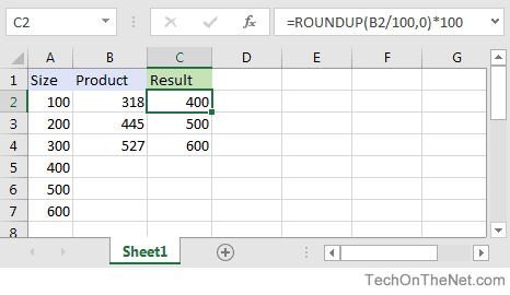
For example in cell C2, you can use the IF function and the ROUNDUP function as follows:

=ROUNDUP(B2/100,0)*100

This will return the correct value of 400 for a value of 318 in cell B2. Just copy this formula to cell C3, C4 and so on.