Excel absolute all cells

By default, a cell reference is a relative reference, which means that the reference is relative to the location of the cell. If, for example, you refer to cell A2 from cell C2, you are actually referring to a cell that is two columns to the left (C minus A)—in the same row (2). When you copy a formula that contains a relative cell reference, that reference in the formula will change.

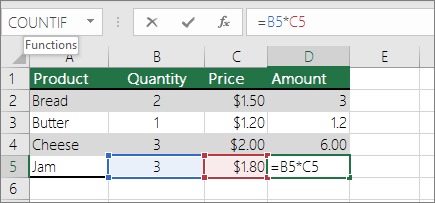
As an example, if you copy the formula =B4*C4 from cell D4 to D5, the formula in D5 adjusts to the right by one column and becomes =B5*C5. If you want to maintain the original cell reference in this example when you copy it, you make the cell reference absolute by preceding the columns (B and C) and row (2) with a dollar sign ($). Then, when you copy the formula =$B$4*$C$4 from D4 to D5, the formula stays exactly the same.

Less often, you may want to mixed absolute and relative cell references by preceding either the column or the row value with a dollar sign—which fixes either the column or the row (for example, $B4 or C$4).

To change the type of cell reference:

1. Select the cell that contains the formula.

2. In the formula bar , select the reference that you want to change.

3. Press F4 to switch between the reference types.

   The table below summarizes how a reference type updates if a formula containing the reference is copied two cells down and two cells to the right.

For a formula being copied:	If the reference is:	It changes to:
	$A$1 (absolute column and absolute row)	$A$1 (the reference is absolute)
	A$1 (relative column and absolute row)	C$1 (the reference is mixed)
	$A1 (absolute column and relative row)	$A3 (the reference is mixed)
	A1 (relative column and relative row)	C3 (the reference is relative)

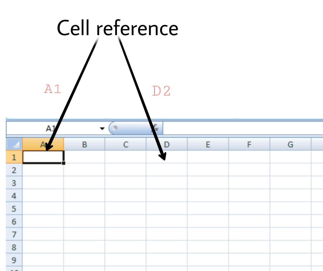
A worksheet in Excel is made up of cells. These cells can be referenced by specifying the row value and the column value.

For example, A1 would refer to the first row (specified as 1) and the first column (specified as A). Similarly, B3 would be the third row and second column.

The power of Excel lies in the fact that you can use these cell references in other cells when creating formulas.

Now there are three kinds of cell references that you can use in Excel:

• Relative Cell References
• Absolute Cell References
• Mixed Cell References

Understanding these different types of cell references will help you work with formulas and save time (especially when copy-pasting formulas).

What are Relative Cell References in Excel?

Let me take a simple example to explain the concept of relative cell references in Excel.

Suppose I have a data set shown below:

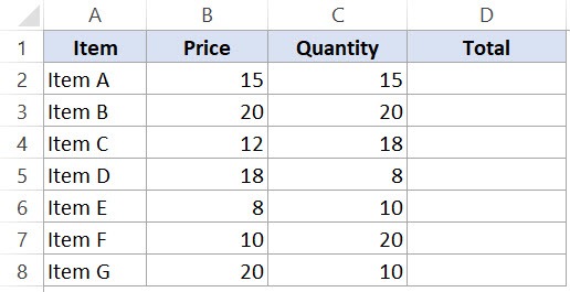
To calculate the total for each item, we need to multiply the price of each item with the quantity of that item.

For the first item, the formula in cell D2 would be B2* C2 (as shown below):

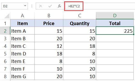
Now, instead of entering the formula for all the cells one by one, you can simply copy cell D2 and paste it into all the other cells (D3:D8). When you do it, you will notice that the cell reference automatically adjusts to refer to the corresponding row. For example, the formula in cell D3 becomes B3*C3 and the formula in D4 becomes B4*C4.

These cell references that adjust itself when the cell is copied are called relative cell references in Excel.

When to Use Relative Cell References in Excel?

Relative cell references are useful when you have to create a formula for a range of cells and the formula needs to refer to a relative cell reference.

In such cases, you can create the formula for one cell and copy-paste it into all cells.

What are Absolute Cell References in Excel?

Unlike relative cell references, absolute cell references don’t change when you copy the formula to other cells.

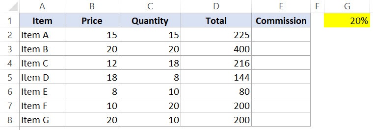
For example, suppose you have the data set as shown below where you have to calculate the commission for each item’s total sales.

The commission is 20% and is listed in cell G1.

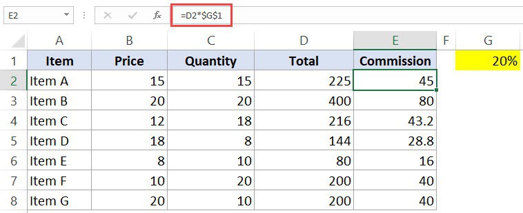
To get the commission amount for each item sale, use the following formula in cell E2 and copy for all cells:

=D2*$G$1

Note that there are two dollar signs ($) in the cell reference that has the commission – $G$2.

What does the Dollar ($) sign do?

A dollar symbol, when added in front of the row and column number, makes it absolute (i.e., stops the row and column number from changing when copied to other cells).

For example, in the above case, when I copy the formula from cell E2 to E3, it changes from =D2*$G$1 to =D3*$G$1.

Note that while D2 changes to D3, $G$1 doesn’t change.

Since we have added a dollar symbol in front of ‘G’ and ‘1’ in G1, it wouldn’t let the cell reference change when it’s copied.

Hence this makes the cell reference absolute.

When to Use Absolute Cell References in Excel?

Absolute cell references are useful when you don’t want the cell reference to change as you copy formulas. This could be the case when you have a fixed value that you need to use in the formula (such as tax rate, commission rate, number of months, etc.)

While you can also hard code this value in the formula (i.e., use 20% instead of $G$2), having it in a cell and then using the cell reference allows you to change it at a future date.

For example, if your commission structure changes and you’re now paying out 25% instead of 20%, you can simply change the value in cell G2, and all the formulas would automatically update.

What are Mixed Cell References in Excel?

Mixed cell references are a bit more tricky than the absolute and relative cell references.

There can be two types of mixed cell references:

• The row is locked while the column changes when the formula is copied.
• The column is locked while the row changes when the formula is copied.

Let’s see how it works using an example.

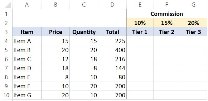
Below is a data set where you need to calculate the three tiers of commission based on the percentage value in cell E2, F2, and G2.

Now you can use the power of mixed reference to calculate all these commissions with just one formula.

Enter the below formula in cell E4 and copy for all cells.

=$B4*$C4*E$2

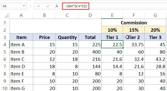
The above formula uses both kinds of mixed cell references (one where the row is locked and one where the column is locked).

Let’s analyze each cell reference and understand how it works:

• $B4 (and $C4) –  In this reference, the dollar sign is right before the Column notation but not before the Row number. This means that when you copy the formula to the cells on the right, the reference will remain the same as the column is fixed. For example, if you copy the formula from E4 to F4, this reference would not change. However, when you copy it down, the row number would change as it is not locked.
• E$2 – In this reference, the dollar sign is right before the row number, and the Column notation has no dollar sign. This means that when you copy the formula down the cells, the reference will not change as the row number is locked. However, if you copy the formula to the right, the column alphabet would change as it’s not locked.

How to Change the Reference from Relative to Absolute (or Mixed)?

To change the reference from relative to absolute, you need to add the dollar sign before the column notation and the row number.

For example, A1 is a relative cell reference, and it would become absolute when you make it $A$1.

If you only have a couple of references to change, you may find it easy to change these references manually. So you can go to the formula bar and edit the formula (or select the cell, press F2, and then change it).

However, a faster way to do this is by using the keyboard shortcut – F4.

When you select a cell reference (in the formula bar or in the cell in edit mode) and press F4, it changes the reference.

Suppose you have the reference =A1 in a cell.

Here is what happens when you select the reference and press the F4 key.

• Press F4 key once: The cell reference changes from A1 to $A$1 (becomes ‘absolute’ from ‘relative’).
• Press F4 key two times: The cell reference changes from A1 to A$1 (changes to mixed reference where the row is locked).
• Press F4 key three times: The cell reference changes from A1 to $A1 (changes to mixed reference where the column is locked).
• Press F4 key four times: The cell reference becomes A1 again.

You May Also Like the Following Excel Tutorials:

• How to Copy and Paste Formulas in Excel without Changing Cell References
• How to Lock Cells in Excel.
• Excel Freeze Panes: Use it to Lock Row/Column Headers.
• How to Lock Formulas in Excel.
• How to Reference Another Sheet or Workbook in Excel
• How to Find Circular Reference in Excel
• Using A1 or R1C1 Reference Notation in Excel (& How to Change These)

Cell reference is the address or name of a cell or a range of cells. It is the combination of column name and row number. It helps the software to identify the cell from where the data/value is to be used in the formula. We can reference the cell of other worksheets and also of other programs.

• Referencing the cell of other worksheets is known as External referencing.
• Referencing the cell of other programs is known as Remote referencing.

There are two types of cell references in Excel:  

• Relative reference
• Absolute reference

Relative Reference

Relative reference is the default cell reference in Excel. It is simply the combination of column name and row number without any dollar ($) sign. When you copy the formula from one cell to another the relative cell address changes depending on the relative position of column and row. C1, D2, E4, etc are examples of relative cell references. Relative references are used when we want to perform a similar operation on multiple cells and the formula must change according to the relative address of column and row.

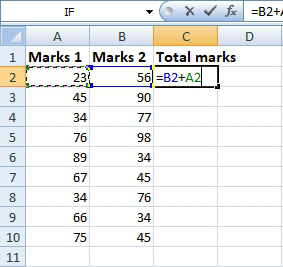
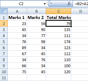
For example, We want to add the marks of two subjects entered in column A and column B and display the result in column C. Here, we will use relative reference so that the same rows of column’s A and B are added.

Steps to Use Relative Reference:

Step 1: We write the formula in any cell and press enter so that it is calculated. In this example, we write the formula(= B2 + A2) in cell C2 and press enter to calculate the formula.

Step 2: Now click on the Fill handle at the corner of cell which contains the formula(C2).

Step 3: Drag the Fill handle up to the cells you want to fill. In our example, we will drag it till cell C10.

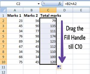
Step 4: Now we can see that the addition operation is performed between the cell A2 and B2, A3 and B3 and so on.

Step 5: You can double-click on any cell to check that the operation is performed in between which cells.

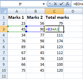
Thus, in the above example, we see that the relative address of cell A2 changes to A3, A4, and so on, similarly the relative address changes for column B, depending on the relative position of the row.

Absolute Reference

Absolute reference is the cell reference in which the row and column are made constant by adding the dollar ($) sign before the column name and row number. The absolute reference does not change as you copy the formula from one cell to other. If either the row or the column is made constant then it is known as a mixed reference. You can also press the F4 key to make any cell reference constant. $A$1, $B$3 are examples of absolute cell reference.

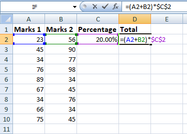
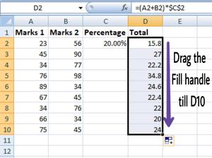
For example, We want to multiply the sum of marks of two subjects, entered in column A and column B, with the percentage entered in cell C2 and display the result in column D. Here, we will use absolute reference so that the address of cell C2 remains constant and does not change with the relative position of column and rows.

Steps to Use Absolute Reference:

Step 1: We write the formula in any cell and press enter so that it is calculated. In this example, we write the formula(=(A2+B2)*$C$2) in cell D2 and press enter to calculate the formula.

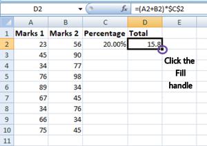
Step 2: Now click on the Fill handle at the corner of cell which contains the formula(D2).

Step 3: Drag the Fill handle up to the cells you want to fill. In our example, we will drag it till cell D10.

Step 4: Now we can see that the percentage is calculated in column D.

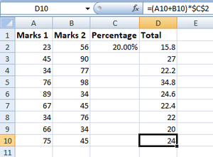
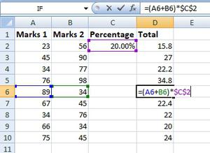
Step 5: You can double-click on any cell to check that the operation is performed in between which cells, and we see that the address of cell C2 does not change.

Thus, in the above example we see that the address of cell C2 is not changed whereas the address of column A and B changes with the relative position of the row and column, this happened because we used the absolute address of the cell C2.

Lock data locations in a formula with this Excel cell reference

Updated on March 14, 2021

What to Know

• To calculate multiple items based on cells elsewhere, and keep the row or column constant, use an absolute cell reference.
• In this equation, the absolute cell reference is A$12: =+B2+B2+A$12.
• The $ symbol «holds» the row or column constant even when copying or filling a column or row with the same formula.

This article explains how to use an absolute cell reference in Excel 2010 and later to prevent formulas from automatically adjusting relative to how many rows or columns you’ve filled.

What Is an Absolute Cell Reference in Excel?

There are two types of ways to reference a cell inside a formula in Excel. You can use a relative cell reference or an absolute cell reference.

• Relative cell reference: A cell address which doesn’t contain the $ symbol in front of the row or column coordinates. This reference will automatically update the column or cell relative to the original cell when you fill either down or across.
• Absolute cell reference: A cell address which contains the $ symbol either in front of the row or column coordinates. This «holds» the reference row or column constant even when filling a column or row with the same formula.

Cell referencing can seem like an abstract concept to those who are new to it.

How to Use Absolute Cell Reference in Excel

There are a few different ways to use an absolute reference in Excel. The method you use depends which part of the reference you want to keep constant: the column or the row.

1. For example, take a spreadsheet where you wanted to calculate actual sales tax for multiple items, based on reference cells elsewhere in the sheet.

2. In the first cell, you’d enter the formula using standard relative cell references for the item prices. But to pull in the correct sales tax into the calculation, you’d use an absolute reference for the row, but not for the cell.

3. This formula references two cells in different ways. B2 is the cell to the left of the first sales tax cell, relative to the position of that cell. The A$12 reference points to the actual sales tax number listed in A12. The $ symbol will keep the reference to row 12 constant, regardless of which direction you fill adjacent cells. Fill all the cells under this first one to see this in action.

4. You can see that when you fill the column, the cell in the second column uses relative cell referencing for the cost values in column B, incrementing the column to match the sales tax column. However the reference to A12 stays constant due to the $ symbol, which keeps the row reference the same. Now fill the D column starting from the C2 cell.

5. Now, you can see that filling the row to the right uses the correct state sales tax (Indiana) because the column reference is relative (it shifts one to the right just like the cell you’re filling). However, the relative reference for cost has now also shifted one to the right, which is incorrect. You can fix this by making the original formula in C2 reference the B column with an absolute reference instead.

6. By placing a $ symbol in front of «B», you’ve created an absolute reference for the column. Now when you fill to the right, you’ll see that the reference to the B column for cost remains the same.

7. Now, when you fill the D column down, you’ll see that all relative and absolute cell references work exactly the way you intended.

8. Absolute cell references in Excel are critical for controlling which cells are referenced when you fill columns or rows. Use the $ symbol however you need within the cell reference to keep either the row or the column reference constant, in order to reference the correct data in the correct cell. When you combine relative and absolute cell references like this, it’s called a mixed cell reference.

   If you use a mixed reference, it’s important to align the column or row of the source data with the column or row where you’re typing the formula. If you’ve made the row reference relative, then keep in mind that when you fill to the side, the column number of the source data will increment along with the column of the formula cell. This is one of the things that makes relative and absolute addressing complicated for new users, but once you learn it, you will have much more control over pulling source data cells into your formula cell references.

Using Absolute Cell References to Pin One Cell Reference

Another approach to using absolute cell referencing is by applying it to both the column and the row to essentially «pin» the formula to use only one single cell no matter where it is.

Using this approach, you can fill to the side or down and the cell reference will always stay the same.

Using an absolute cell reference on both column and row is only effective if you’re only referencing a single cell across all the cells you’re filling.

1. Using the same example spreadsheet from above, you can reference only the single state tax rate by adding the $ symbol to both the column and the row reference.

2. This makes both the «A» column and the «12» row stay constant, no matter what direction you fill the cells. To see this in action, fill the entire column for ME sales tax after you’ve updated the formula with the absolute column and row reference. You can see that each filled cell always uses the $A$12 absolute reference. Neither the column or the row changes.

3. Use the same formula for the Indiana sales tax column, but this time use the absolute reference for both column and row. In this case that’s $B$12.

4. Fill this column, and again you’ll see that the reference to B12 doesn’t change in ever cell, thanks to the absolute reference for both column and row.

5. As you can see, there are multiple ways you can use absolute cell references in Excel to accomplish similar tasks. What absolute references provide you is the flexibility to maintain constant cell references even when you’re filling a large number of columns or rows.

   You can cycle through relative or absolute cell references by highlighting the reference and then pressing F4. Every time you press F4, the absolute reference will be applied to either the column, the row, both the column and cell, or neither of them. This is a simple way to modify your formula without having to type the $ symbol.

When You Should Use Absolute Cell References

Throughout nearly every industry and field, there are a lot of reasons you may want to use absolute cell references in Excel.

• Using fixed multipliers (like price per unit) in a large list of items.
• Apply a single percentage for each year when you’re projecting annual profit targets.
• When creating invoices, use absolute references to refer to the same tax rate across all items.
• Use absolute cell references in project management to refer to fixed availability rates for individual resources.
• Use relative column references and absolute row references to match column calculations in your referenced cells to column values in another table.

If you do use a combination of relative and absolute references for columns or rows, you just need to make sure that the position of the source data columns or rows match the column or row of the destination cells (where you’re typing the formula).

Thanks for letting us know!

Get the Latest Tech News Delivered Every Day

Subscribe

One of the first things we learn in Excel is the magic of the $ symbol. It freezes the row or column, so the cell reference does not change when copying a formula. This is known as an absolute reference. With the introduction of Tables came a different (and more semantic) way to reference cells, called structured references. However, structured references don’t follow the same principles as the standard A1 style referencing system we usually use. As a result, the $ symbol approach won’t work. But don’t worry; by the end of this post, you will know how to create an Excel Table absolute reference.

Download the example file: Click the link below to download the example file used for this post:

Watch the video

Watch on YouTube

Scenario

The examples in this post all use the following Table.

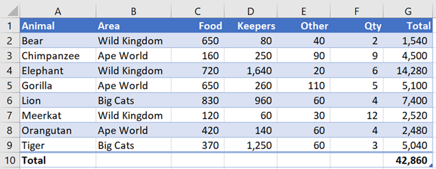
The Table shows the costs a Safari Park might incur for owning different types of animals. The Table name is myTable, whilst it’s not a great name, it will work for this example.

When using structured references, whole columns are referenced with this syntax:

tableName[columnName]

Using the example data to sum the Total column, the formula would be:

=SUM(myTable[Total])

If this were dragged or copied to another column, the formula would change automatically. If copied to the left, it would change to:

=SUM(myTable[Qty])

If copied to the right, it would revert to the first column in the table and changes to:

=SUM(myTable[Animal])

NOTE: This is one of the quirks when working with Table columns. Once a structured column reference reaches the end of the Table, it loops back to the start.

If using the standard A1 style referencing, we could add the $ signs and change the range from G2:G9 (a relative reference) to $G$2:$G$9 (an absolute reference). But we can’t use $ with the structured references found in Tables.

To achieve the same result, we need to add more square brackets, a colon ( : ), and repeat the column name.

=SUM(myTable[[Total]:[Total]])

The difference between the relative and absolute reference for columns is shown in blue above.

If you have been using Tables for a while, you will notice this is the same syntax as when referencing multiple columns.

=SUM(myTable[[Food]:[Other]])

The reference above shows how to sum the columns from Food to Other in the example data. This means multi-column references selected using the mouse are absolute by default. 

To create a relative multi-column reference, we need to remove the outer square brackets and repeat the table name, as shown below.

=SUM(myTable[Food]:myTable[Other])

Or you could include each column individually within the calculation as shown below, which achieves the same result.

=SUM(myTable[Food],myTable[Keepers],myTable[Other])

Relative and absolute reference for cells in the same row

When using Tables, the syntax to reference a cell in the same row is as follows.

=[@Total]    or    =[@[Total Value]]

NOTE: the 2nd syntax in the example above is where the header contains a space or special character.

If the formula is contained in a cell outside the Table, the Table name must also be added:

=myTable[@Total]    or    =myTable[@[Total Value]

To make a row reference absolute, the same principles apply as we saw for column references. It does not matter if the reference is inside or outside the Table; the Table name is required for both.

=myTable[@[Total]:[Total]]

To reference multiple columns, the syntax is similar.

=SUM(myTable[@[Food]:[Other]])

The reference above shows how to sum the columns from Food to Other from the example data. This is an absolute column reference.

To create a relative multi-column reference, we need to remove the outer square brackets.

=SUM([@Food]:[@Other])    or    =SUM(myTable[@Food]:myTable[@Other])

NOTE: The @ symbol serves the same purpose as when working with dynamic arrays; it calculates based on the implicit intersection. Check out this post for more information: Dynamic arrays in Excel

Relative and absolute reference for any cell

In the section above, we considered the scenario where the column was absolute while the row was based on a cell in the same row. However, to reference a row which is not in the same row different approach.

The INDEX function returns a cell reference or value from a specified location in a range or array. As a simple example, look at the following formula:

=INDEX($G$2:$G$9,1)

This formula would always return the first row from cells G2:G9. To return the second cell from the same range, the formula would be

=INDEX($G$2:$G$9,2)

Therefore, using INDEX with structured references allows us to refer to any individual cell in the range. For example, the following returns the first item from the Total column.

=INDEX(myTable[Total],1)

Tow is an absolute reference, but the column is relative; therefore this is a mixed reference.

To create a full relative reference, we must also find a way to count row numbers within the INDEX.

The following uses ROW(A1) to calculate a relative row reference. ROW(A1) evaluates to 1. When dragged down, ROW(A2) evaluates to 2. Therefore ROW creates the relative number to use in the INDEX function.

=INDEX(myTable[Total],ROW(A1))

The formula above is a fully relative table reference.

Absolute references in Headers and Totals

Referencing the Header and Total rows within a Table is slightly different again. This is because Headers and Totals inherently have absolute row references but not column references.

The relative reference for Headers is shown below:

=myTable[[#Headers],[Food]]

To turn the Header reference into an absolute reference, add the section highlighted below.

=myTable[[#Headers],[Food]:[Food]]

If you’ve read this post all the way through, then the multi-column absolute reference will not surprise you. The formula to count the column headings is shown below.

=COUNTA(myTable[[#Headers],[Food]:[Other]])

And the multi-column relative reference will not surprise you either.

=COUNTA(myTable[[#Headers],[Food]]:myTable[[#Headers],[Other]])

The examples in this section all include the Header row (#Headers). To reference the Total row, use #Totals instead.

Conclusion

With a Table, the different syntax to provide relative or absolute references can be quite subtle. An @ or square bracket out of place can cause an error that can be incredibly frustrating to find. It is easier to start with a valid reference and then adjust it, rather than typing the reference from scratch.

As with all things, practice is vital. Before long, creating an Excel Table absolute reference will be second nature.

Related posts:

• Running total in an Excel Table
• How to use Excel Table within a data validation list (3 ways)